Semiparametric Estimation of the Relationship between ROC Operating Points and the Test-result Scale

Abstract

Rationale and Objectives

Semiparametric methods provide smooth and continuous receiver operating characteristic (ROC) curve fits to ordinal test results and require only that the data follow some unknown monotonic transformation of the model's assumed distributions. The quantitative relationship between cutoff settings or individual test-result values on the data scale and points on the estimated ROC curve is lost in this procedure, however. To recover that relationship in a principled way, we propose a new algorithm for “proper” ROC curves and illustrate it by use of the proper binormal model.

Materials and Methods

Several authors have proposed the use of multinomial distributions to fit semiparametric ROC curves by maximum-likelihood estimation. The resulting approach requires nuisance parameters that specify interval probabilities associated with the data, which are used subsequently as a basis for estimating values of the curve parameters of primary interest. In the method described here, we employ those “nuisance” parameters to recover the relationship between any ordinal test-result scale and true-positive fraction, false-positive fraction, and likelihood ratio. Computer simulations based on the proper binormal model were used to evaluate our approach in estimating those relationships and to assess the coverage of its confidence intervals for realistically sized datasets.

Results

In our simulations, the method reliably estimated simple relationships between test-result values and the several ROC quantities.

Conclusion

The proposed approach provides an effective and reliable semiparametric method with which to estimate the relationship between cutoff settings or individual test-result values and corresponding points on the ROC curve.

A receiver operating characteristic (ROC) curve is a continuous curve that plots sensitivity, often called true-positive fraction (TPF), as a function of 1 – specificity, here called false-positive fraction (FPF), and has become one of the primary tools used to assess the performance of diagnostic tests that classify individuals into two groups (1–3). During initial phases of a clinical evaluation of such tests, the focus is often on the ROC curve itself rather than upon the relationship between test-result values and points on that ROC curve (ie, pairs of TPF and FPF). An ROC curve summarizes the ability of any device or decision process to classify disease in a binary way without reference to the relationship between test-result values to points on the curve. However, when one wants to employ the classifier in a clinical situation, it is necessary to understand how values of the test's quantitative results relate to particular “operating points” on the ROC curve, because a quantitative diagnostic method usually cannot be applied without adopting a particular test-result value as a cutoff to separate domains of distinctly different action (eg, do nothing or order additional tests, as in screening mammography). A closely related but subtly distinct estimation task concerns the position on a given ROC curve at which the test-result value of an individual patient lies, which quantifies the extent to which classification of that particular patient is “easy” or “difficult” for the diagnostic test in question and can serve as a basis for calibrating radiologists’ and/or automated classifiers’ reporting scales. Therefore, this article describes a new approach to the task of estimating the quantitative relationship between individual patients'test-result values and/or various cutoff settings on the test-result scale, on one hand, and position on the corresponding test's ROC curve, on the other.

A concrete example may help to clarify one aspect of our motivation. Consider a computer classifier designed to diagnose breast cancer from mammographic images, the output of which lies on a scale from 0% to 100%, with larger values indicating stronger likelihood of the presence of malignancy. The ROC curve of such a classifier can be estimated from the test results of a sample of patients’ images by any of a variety of methods. However, most methods for ROC curve estimation cannot answer questions such as “What are the classifier's sensitivity and specificity (ie, its ROC operating point) if every breast lesion with a computer output greater than 2% is sent to biopsy?” Here we address this need for “proper” (ie, convex) ROC curves, with primary focus on the proper binormal model.

Our approach is based on an assumption that the test-result values and cutoff values discussed in this article are “ordinal” (eg, larger test-result values are interpreted as more strongly indicative of the presence of the disease in question); however, those values may be either explicit (eg, a fasting plasma glucose level ≥126 mg/dL as the diagnostic criterion for diabetes, according to the World Health Organization) (4) or implicit (eg, when reading mammograms radiologists must report their clinical impression on the BI-RADS [ie, breast imaging reporting and data system] scale, which is essentially an action scale, by use of loosely defined cutoff values) (5). In the following we assume also that the test-result values of interest yield a “proper” ROC curve (ie., a ROC such that curve slope decreases monotonically from left to right, so that the curve is convex, or “concave” in strict mathematical terminology).

Many methods have been proposed to estimate ROC curves and their figures of merit. Approaches used for that purpose usually can be described as parametric, semiparametric (Pepe refers to semiparametric approaches as “parametric distribution-free”) (2) or nonparametric. Parametric models assume that the quantity measured in a study (the decision-variable outcome or test-result value), or some known function of it, arises from a pair of probability distributions with a particular analytical form, usually two normal or logistic distributions, that must be chosen before data analysis. The main weakness of this approach is that decision variables usually do not follow any known distribution, even approximately. In contrast, nonparametric methods do not assume any specific form whatsoever for the distribution of the decision variable—though some such methods may assume weak relationships between, for example, the distribution of the actually positive cases (patients with the condition we are trying to diagnose) and the distribution of the actually negative cases (patients who do not have the condition we are trying to diagnose). Semiparametric models lie between the previous two extremes in the sense that they usually posit only an unknown monotonic relationship between the assumed theoretical distributions in the model and the empirically observed test-result values. This is equivalent to assuming the existence of a latent (unobserved) variable that is monotonically related to the empirical variable in an unknown way. In general, when the assumed distributional form is essentially correct, parametric models are statistically more efficient than semiparametric models, which in turn are more efficient than nonparametric models. However, gains in efficiency are quickly lost and bias is introduced when the mathematical form of the assumed distributional model fails to represent the empirical data population accurately (6). Much experimental evidence suggests that semiparametric methods produce good ROC curve estimates (1,7–11), thereby implying that the existence of a latent variable with an explicit mathematical form usually is a reasonable assumption and that the methods are usefully robust.

As mentioned previously, in addition to estimating a given binary classifier's ROC curve and corresponding indices of accuracy (eg, total and partial areas under the curve), it may be of interest in practical applications of ROC analysis also to estimate the relationship between individual patients’ test-result values and/or various test-result cutoff settings, on one hand, and corresponding values of TPF, FPF, and perhaps likelihood ratio (LR), on the other. Unfortunately, the relationship between test-result values and points on the ROC curve is not estimated when semiparametric models are used to fit an ROC curve, because only test-result ranks are employed to avoid the strong constraints imposed by parametric, rather than semiparametric, models (12–14). If the number of distinct values that test results can adopt (eg, the integers from 1 to 5) is small compared to the number of cases in a test-evaluation study, calculation of the relationship is straightforward: each observed test-result value corresponds to a specific cumulative probability between cutoffs and the indices in question that can be computed accordingly. However, this simple relationship becomes less meaningful as the number of possible test-result values increases. (A number of other potentially problematic issues related to the quantization of scales and discrete ordinal scales in general lie beyond the scope of this manuscript but are addressed elsewhere.) (2,15,16) Although often the scale relationships in question still can be estimated with reasonable accuracy for such data by a mix of curve fitting and nonparametric methods (17), we believe that a more principled approach would estimate the scale relationships within the same framework as the ROC curve. Therefore, we developed a method to estimate the relationship between the original test-result variable and the corresponding latent variable entirely on the basis of the semiparametric approach to ROC curve fitting. In this way, the relationship between test-result values and TPF, FPF, and LR can be recovered uniquely and reproducibly.

In passing, we note that the inverse problem—estimating the threshold associated with a particular operating point—also can be considered. Readers interested in the inverse problem can either apply the same principles described in the following section, which is straightforward but tedious, use a bootstrap-based method as done by Drukker et al (18), or take an approach similar to that of exact confidence intervals (19).

This paper is structured as follows. First, we provide a brief description of the maximum-likelihood estimation (MLE) algorithm that implements our semiparametricmodels. An approach is then proposed for estimation of latent decision-variable, TPF, FPF, and LR valuesand their standard errors. Finally, we describe an initial assessment of our scheme by computer simulation and real data, followed by a discussion of the potential advantages, applications, and limitations of the approach.

MATERIALS AND METHODS

Brief Description of the Ogilvie-Dorfman-Metz Approach to Estimation of ROC Curves

The MLE approach to fitting ROC curves was introduced essentially independently by Ogilvie et al (20) and Dorfman et al (13) and subsequently was extended to continuously distributed data by Metz et al (12). Therefore, we refer to the general method described below as the Ogilvie-Dorfman-Metz approach.

ROC analysis is based inherently on rank order rather than on interval-scale values (2), because an ROC curve plots a cumulative distribution of actually positive cases against a corresponding cumulative distribution of actually negative cases; therefore, it can be applied to any test-result data that can be ordered (ie, are “ordinal”). The measurements used in diagnostic medicine range from inherently categorical, where only a few distinct ordinal values are possible (usually much fewer than the dataset's size), to quasi-continuous, where a larger though finite number of digits is observed and stored, leading to few if any tied values in the rating data. For example, recording probability estimates from an artificial neural network by using 4 decimal digits, starting from 0.0000 and ending with 1.0000, provides 10,001 possible values; thus, quasi-continuous data are equivalent to ordinal category data with a large number of categories (1, 2, 3 ...M_tot). Starting from this observation, Metz et al (12) showed that test-result data can be replaced by a set of “truth-state runs” (sequences of rank-ordered test results with the same truth, either actually negative or actually positive) without affecting the maximum-likelihood estimates of the curve parameters. This procedure often produces a dataset with a much smaller set of categories, M<<M_tot, such that each category is populated, thereby rendering implementations faster and more reliable.

Following this procedure, only categorical data need be considered. A categorical dataset is described fully by the number of responses in each category for a study's N₀ actually negative cases (ie, class 0, in a two-class decision process):

$${\overrightarrow{n}}_0\equiv \left\{n_{0,1},n_{0,2},\dots ,n_{0,M}\mid \sum _i{n}_{0,i}=N_0\right\}$$

and for its N₁ actually positive cases (class 1):

$${\overrightarrow{n}}_1\equiv \left\{n_{1,1},n_{1,2},\dots ,n_{1,M}\mid \sum _i{n}_{1,i}=N_1\right\}.$$

If the test results are mutually independent, then the likelihood of obtaining a particular combination of outcomes in the M-occupied categories can be modeled with independent multinomial distributions for the actually negative and actually positive cases. In MLE calculations one usually employs the log-likelihood function for both practical and theoretical reasons (21), yielding:

$$LLR\propto \sum _{i=1,M}{n}_{0,i}\log p_{0,i}+\sum _{i=1,M}{n}_{1,i}\log p_{1,i}$$ (1)

where p_0,i and p_1,i are the probabilities associated with category i for the negative and positive distributions, respectively. These probabilities can be defined for a semiparametric model via the equations

$$p_{0,i}=P\left(x_{i-1}<x\le x_i\mid \alpha ,\beta ,-\right)$$ (2)

$$p_{1,i}=P\left(x_{i-1}<x\le x_i\mid \alpha ,\beta ,+\right),$$ (3)

in which the parameters α and β specify a particular member of the population-model family (usually only two parameters are employed, to avoid overfitting) and $\overrightarrow{x}$ is a vector of ordinal category boundaries (“cutoffs”) on the latent decision-variable scale, x. Notice that each conditional-probability vector contains M-1 elements, because p_0,M and p_1,M are completely defined by its previous M-1 values, given that probabilities must sum to 1. Thus, the pairs (p_0;i; p_1;i) are given by

$$P\left(x_{i-1}<x\le x_i\mid \alpha ,\beta ,-\right)={\int }_{x_{i-1}}^{x_i}{f}_x\left(x\mid \alpha ,\beta ,-\right)dx$$

and

$$P\left(x_{i-1}<x\le x_i\mid \alpha ,\beta ,+\right)={\int }_{x_{i-1}}^{x_i}{f}_x\left(x\mid \alpha ,\beta ,+\right)dx,$$

respectively, where f_x(x|α, β, –) and f_x(x|α, β, +) are the model's probability density functions for actually negative and actually positive cases, respectively. The task of maximum-likelihood estimation is to calculate the values of the parameters α and β that maximize Equation 1. From this point forward, we use the term MLE to indicate the Ogilvie-Dorfman-Metz semiparametric approach unless otherwise specified.

Estimation of the Relationship between the Test-Result and the Latent Variable

Metz et al (12) showed that estimates of the cutoffs that bound the truth-runs can be used either to estimate unequivocally the cutoff that lies between each of the distinct values present in the truth-runs or to summarize a set of those values if the number of truth-runs must be limited to ensure numerical stability (12). The latter concern appears to be unnecessary with stable estimation algorithms (eg, the one described by Pesce and Metz) (11) and will not be discussed hereafter. According to any semiparametric model, each value on the test-result scale and a corresponding value on the latent scale are associated with the same statistical event (21) if the relationship is one-to-one, as is the case for any proper model. This means that the latent-scale distribution defined for x_i–1<x≤x_i by Equations 2 and 3 can describe, after some monotonic transformation, the statistics of the test-result value, t_i, that is associated with category i as well. However, it is important to recognize that although the cutoffs represent values that separate different categories on the latent scale, data values on the test-result scale represent values within such categories. Therefore the correspondence between the two kinds of values is complementary rather than direct. We propose to estimate this complementary relationship within each category in terms of either the expected or the median value within an interval between adjacent cutoffs on the latent scale (ie, in terms of either the mean)

$$\widehat{x}\left(t_i\right)={\stackrel{‒}{x}}_i\equiv \frac{n_{0,i}}{n_{0,i}+n_{1,i}}{\int }_{x_{i-1}}^{x_i}x{f}_x\left(x\mid \alpha ,\beta ,-\right)dx∕{\int }_{x_{i-1}}^{x_i}{f}_x\left(x\mid \alpha ,\beta -\right)dx+\frac{n_{1,i}}{n_{0.i}+n_{i,1}}{\int }_{x_{i-1}}^{x_i}x{f}_x\left(x\mid \alpha ,\beta ,+\right)dx∕{\int }_{x_{i-1}}^{x_i}{f}_x\left(x\mid \alpha ,\beta ,+\right)dx$$ (4a)

or the median

$$\widehat{x}\left(t_i\right)={\tilde{x}}_i\equiv {\mu }_{1∕2}\left\{\frac{n_{0,i}}{n_{0,i}+n_{1,i}}{f}_x\left(x\mid \alpha ,\beta ,-\right)+\frac{n_{1,i}}{n_{0,i}+n_{1,i}}{f}_x\left(x\mid \alpha ,\beta ,+\right)\mid x_{i-1}<x<x_i\right\},$$ (4b)

where μ_1/2{f(x)|R} indicates the median of any probability density f(x) within the range R, and where x₀ and x_M are defined as – ∞ and + ∞, respectively. The density in curly braces in Equation 4b is the estimate of the population mixture distribution that is associated with the conditional densities f_x(x|α,β,–) and f_x(x|α,β,+) within the interval x_i < x < x_i-1.

To define the complimentary relationship between a particular test-result value t_i and the corresponding log-likelihood ratio (LLR), we again use either the median or the mean. Use of median has the advantage that e^{(median of LLR)} in any interval of x is simply the median of LR, so working with LR or LLR is essentially equivalent. With the median, we also can exploit the fact that, for a convex ROC curve, the median value of LLR within any interval of the latent decision-variable scale x must be the LLR of the median x (because LLR and x are then monotonically related) to compute

$$LLR\left(t_i\right)=LL{R}_i=LLR\left({\tilde{x}}_i\right),$$ (5)

where LLR(x̃_i) is determined analytically by the model. However, the mean of LLR is not the LLR of the mean, so when means are used to define the complimentary relationship between test-result and LLR, the mean value of LLR must be computed directly from the mixture distribution of the latent variable between the estimated cutoffs:

$$LLR\left(t_i\right)=LL{R}_i\equiv \frac{n_{0,i}}{n_{0,i}+n_{1,i}}{\int }_{x_{i-1}}^{x_i}LLR\left(x\right)f_x\left(x\mid \alpha ,\beta ,-\right)dx∕{\int }_{x_{i-1}}^{x_i}{f}_x\left(x\mid \alpha ,\beta ,-\right)dx+\frac{n_{1,i}}{n_{0,i}+n_{i,1}}{\int }_{x_{i-1}}^{x_i}LLR\left(x\right)f_x\left(x\mid \alpha ,\beta ,+\right)dx∕{\int }_{x_{i-1}}^{x_i}{f}_x\left(x\mid \alpha ,\beta ,+\right)dx.$$ (6)

When the semiparametric model employed is the proper binormal model, the performance of the algorithm based on median values (Equation 5) to determine the complimentary relationship between test-result and LLR was found, as we shall see, to be essentially identical to that based on mean values (Equation 6). Because using the median value is computationally more efficient, we focus hereafter on median values.

Finally, to define the complimentary relationship between the test result and TPF and FPF, we use

$$\begin{array}{cc}\hfill TPF\left(t_i\right)& \equiv TPF\left({\tilde{x}}_i\right)\hfill \\ \hfill FPF\left(t_i\right)& \equiv FPF\left({\tilde{x}}_i\right),\hfill \end{array}$$ (7)

where, as was the case with LLR, TPF(t_i) and FPF(t_i) are determined analytically from the median value within a range on the latent scale of an assumed model. Note that the operating point (FPF(t_i), TPF(t_i)) lies on the estimated ROC curve, and that LLR(t_i) is the natural (Napierian) logarithm of the slope of the estimated curve at that point.

Standard errors for the estimates of TPF, FPF, and LLR can be estimated by the delta method (22), with derivatives of the likelihood function with respect to various parameters obtained either numerically or analytically. The variance-covariance matrix of the MLE parameter estimates is determined already by our PROPROC software that fits ROC curves semiparametrically on the basis of the proper binormal model (11) and is computed according to the standard approach used in such MLE calculations (13) (ie, by use of the Cramer-Rao bound that is given by the inverse of the negative expected Hessian of the log-likelihood function) (22).

We derived and calculated the relationship between test results and LLRs for the proper binormal model in terms of both median and mean values. All of the mathematical expressions needed for that purpose were solved analytically when possible and checked numerically. Software that implements them is available without charge from our website (http://rocweb.bsd.uchicago.edu/MetzROC). FPF and TPF were calculated only for the median values because we saw little point in estimating FPF and TPF pairs that did not lie on the estimated ROC curve and because the previously implemented LLR and test-result estimates showed little or no difference between the two approaches.

Description of the Simulation Studies

We simulated test-result data with a known monotonic relationship to TPF, FPF, and LLR and then evaluated the estimates of our algorithm against these known relationships. In all simulation studies, the simulated test-result values were based on the latent decision variable, v, of the proper binormal model (23), which is related to LLR by the monotonic relationship

$$v=\frac{(b+1)y}{a+\sqrt{a^2+2(1-b^2)y}},$$ (8)

where

$$y=LLR-\log \left(b\right)$$ (9)

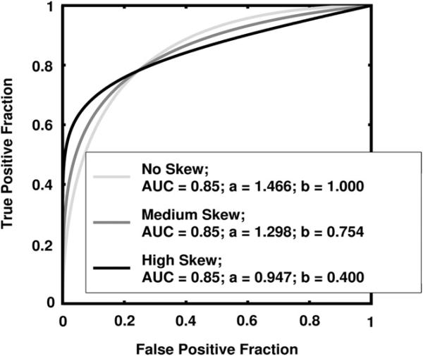
and where a and b are the conventional binormal parameters (2). (Notice that we are expressing the proper binormal model here in terms of the conventional binormal parameters a and b rather than the usual proper-binormal parameters d_a and c, because doing so simplifies this discussion somewhat; however, readers must keep in mind that we are discussing the proper binormal model here.) From each of three population density pairs, the binormal parameters and ROC curves of which are shown in Figure 1, we generated 5000 datasets of 200, 300, 400, and 1000 values of v. The skewed curves that we simulated cling only to the FPF = 0 axis rather than to the TPF = 1 axis because previous simulation studies showed that curves clinging to TPF = 1 behave identically due to model symmetries (11), as expected. The prevalence of actually positive cases was 50% for each simulated dataset. For each input test-result value, our algorithm estimated the corresponding TPF, FPF, and LLR values together with the uncertainties of these estimates.

Figure 1.

The receiver operating characteristic (ROC) curves, binormal parameters, and areas under the ROC curve (AUCs) for the three populations used in the simulation studies.

Because a monotonic transformation of each simulated test-result value v is linearly related to the actual LLR via Equations 8 and 9, we used linear regression to evaluate our estimation of the mathematical relationship between the LLR and the test result. That is, from the simulated test-result values of v, we computed

$$y=\frac{2v(a+(1-b)v)}{1+b},$$

which is the inverse of Equation 8. Thus, the transformed test-result values are linearly related to the true LLR by Equation 9, so linear regression of the transformed test-result values y and estimated LLR produced estimates of the regression slope and intercept with true values 1 and -log(b), respectively. Note that in this case a linear relationship is the true model rather than an approximation. We used both ordinary and weighted least squares regression, with the reciprocal of the errors on the estimated LLR provided by the delta method as weights in the latter.

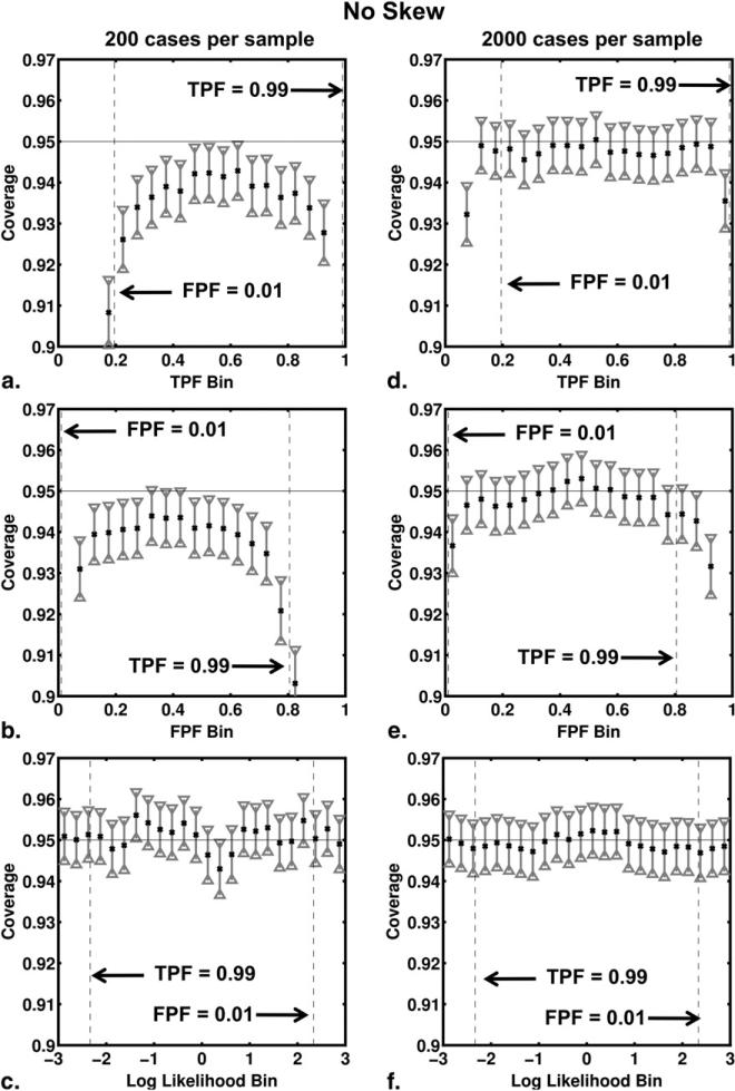
We also investigated the coverages of the 95% confidence intervals (CIs) for our TPF, FPF, and LLR estimates. The coverage of a CI is the proportion of dataset outcomes for which the statistically variable CIs calculated from individual datasets contain the fixed true value of interest. Because the 95% CI for an estimate is expected to contain the true value 95% of the time, the coverage of that CI in a large number of trials should be close to 95% if the assumptions used to construct the 95% CI are correct. In our case, the set of true values of TPF, FPF, and LLR changes with each dataset because the values of v are randomly selected from essentially continuous distributions; therefore, we computed the coverage for the 95% CI of the kth bin of the relevant quantity, which is the proportion of those true values in the kth bin that are also in the 95% CI of the estimated value (eg, see Fig 5). We took the TPF and FPF bin sizes to be 0.05 and the LLR bin size to be 0.25, with these particular bin sizes chosen for plotting clarity. Because coverage is a binomial proportion, we estimated its standard errors by

$$\sigma \left(C_k\right)=\sqrt{\frac{C_k(1-C_k)}{N_k-1}},$$ (10)

where C_k is the coverage for 95% CI of the kth bin and N_k is the number of datasets with at least one true value in the kth bin. This choice of N_k derives from two observations. If many corresponding true values fall into a particular bin for a given dataset of v values, then the corresponding estimated values of FPF, TPF, and LLR will be highly correlated, so care must be taken to ensure that the large number of such highly correlated values does not overly effect (and therefore bias) the error estimate provided by Equation 10, which implicitly assumes independent events. On the other hand, if none of the corresponding true values fall into a particular bin for a given data-set of v values, then that dataset should not be counted in the error estimation.

Figure 5.

Coverage of the 95% CIs for true-positive fraction (TPF), false-positive fraction (FPF), and log-likelihood ratio (LLR) bins for the no-skew receiver operating characteristic curve shown in Figure 1. The coverage results from our simulation studies involving 200 cases per sample are shown in panels (a), (b) and (c), respectively, whereas those of simulation studies involving 2000 cases per sample are shown in panels (d), (e) and (f).

We expected the performance of our algorithm (or any other such algorithm) to decrease for test-result values that correspond to points in ROC space near either the lower-left (FPF = 0, TPF = 0) or upper-right (FPF = 1, TPF = 1) corners, because data outcomes are relatively sparse in these regions, so any algorithm requires relatively extensive interpolation and extrapolation. Fortunately, such points also lie outside the region of ROC space that tends to be clinically relevant. In this paper we focus on the performance of our algorithm in estimating TPF, FPF, and LLR for test result values that correspond to points in ROC space between TPF = 0.99 and FPF = 0.01.

Description of the Real-data Analysis

In addition to the simulations described previously, we used our model-based algorithm to estimate TPF and FPF for real data taken from the computer diagnosis of breast lesions imaged by ultrasound. With a dataset of ultrasound images of 1251 lesions (212 biopsy-confirmed cancers), we performed a leave-one-case-out analysis using a linear discriminant analysis classifier to merge four computer-extracted features. A description of the features and their extraction are described elsewhere (24–27); here we refer to the output of the leave-one-case-out analysis simply as the output. Using our model-based algorithm, we estimated the output thresholds, t_TPF=0.90 and t_FPF=0.10, corresponding to TPF = 0.90 and FPF = 0.10, respectively. These two conditions on TPF and FPF were chosen as representing conditions of high sensitivity (TPF = 0.90) and high specificity (FPF = 0.10) for a breast cancer diagnostic analysis.

To provide a foundation for understanding better how model-based estimates obtained from the real data relate to the associated empirically estimated quantities, two empirical comparisons were performed using post-hoc bootstrapping of the leave-one-out output. In the first, our model-based and empirical estimates of the thresholds t_TPF=0.90 and t_FPF=0.10 were compared. For each of 5000 bootstrap samples, we counted the fraction of malignant output greater than the threshold (TPF) and the fraction of benign output greater than the threshold (FPF). Empirical estimates of threshold were then determined by taking the median threshold value over the 5000 bootstrap samples, and 95% CIs for the median threshold values were determined by using the bootstrap quantiles (28). In our second comparison, the model-based estimates of operating points in ROC space corresponding to the thresholds t_TPF=0.90 and t_FPF=0.10 were compared to the empirical operating points corresponding to the same thresholds. Post-hoc bootstrapping was applied as described previously.

RESULTS

As noted previously, the performance of the algorithm based on mean values (Equation 6) that we used to determine the complimentary relationship between test results and LLRs was found to be essentially identical to that based on median values (Equation 5); therefore, we report only the results based on median values here.

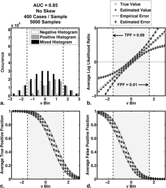
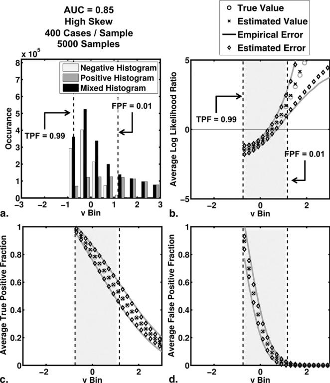
The average behavior of the algorithm in our simulation studies is shown in Figures 2 and 3 for the no-skew and high-skew populations, respectively. Results for the medium-skew population were similar and are available on request. For each bin of test-results, v, we computed the average true and average estimated values of TPF, FPF, and LLR as well as the empirical and average estimated errors on each of TPF, FPF, and LLR. The empirical error for a particular bin is defined here as the standard deviation of estimates in that bin. In each subfigure, we have highlighted the interval of test-result values between those corresponding to TPF = 0.99 and FPF = 0.01. To indicate the number of simulated test-results contained in each LLR bin, we have included also histograms for the actually positive, actually negative and mixed simulated test-result values (5000 samples, each containing 200 positive and 200 negative cases).

Figure 2.

The average behavior of the estimation algorithm (areas under the receiver operating characteristic curve = 0.85 and no skew). (a) Histograms of simulated test-result values (5000 samples of 200 positive and 200 negative cases each) are shown. The negative, positive, and mixed histograms are histograms of the actually negative cases, the actually positive cases, and all cases taken together, respectively. (b,c,d) The results for the average log likelihood ratio, the average true positive fraction and the average false positive fraction, respectively. These averages were taken over bins of test-results, versus the 95% confidence intervals constructed from the average estimated errors and the empirical errors (standard deviation of the distribution of the estimates) are shown also. “Estimated value” here indicates the mean of the samples that belong to that bin.

Figure 3.

The average behavior of the estimation algorithm (areas under the receiver operating characteristic curve = 0.85 and high skew). (a) Histograms of simulated test-result values (5000 samples of 200 positive and 200 negative cases each) are shown. The negative, positive, and mixed histograms are those of the actually negative cases, the actually positive cases, and all cases taken together, respectively. (b,c,d) The results for average log likelihood ratio, average true-positive fraction, and average false-positive fraction, respectively. These averages were taken over bins of test-results. Also shown are 95% CIs constructed from the average estimated errors and the empirical errors (standard deviation of the distribution of the estimates).

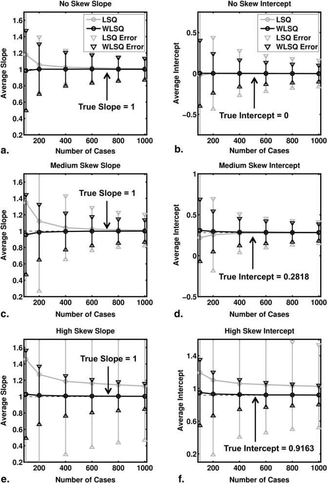
The results of our regression analyses are shown in Figure 4. Note that the true slope is 1 (regardless of the values of a and b) in the linear relationship between y and LLR (Equation 8), whereas the true intercept is -log(b). Use of weighted least squares for the regression resulted in smaller errors and biases than use of ordinary least squares. The difference between the ordinary and weighted least-squares results is most evident for the high-skew ROC curve.

Figure 4.

Results of the regression analysis. Averages were taken over 5000 samples of 100, 200, 400, 600, 800, and 1000 cases each. The 95% confidence intervals constructed from the standard errors are shown also. (a,c,e) The average estimated slope for the no-, medium-, and high-skew ROC curves, respectively. Similarly (b,d,f) depict the average estimated intercept. Results based on ordinary and weighted least squares results are labeled least squares (LSQ) and weighted least squares (WLSQ), respectively. Please note that although the ranges of the vertical axes of Figs 4b, d, and f differ, each spans 1.5 units.

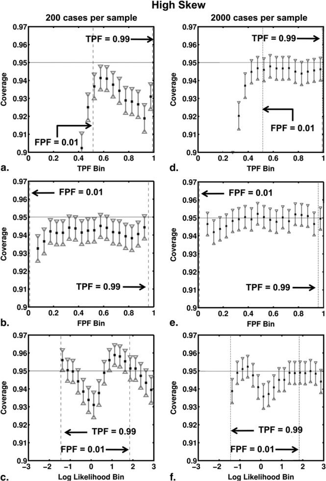
Figures 5 and 6 show the results of the coverage analysis for the no-skew and high-skew simulations, with both 200 and 2000 cases per sample. The coverage and its 95% CI are shown for each TPF, FPF, and LLR bin. As expected, the coverage results for TPF, FPF and LLR improved in both no-skew and high-skew simulations when the number of cases per sample increased from 200 to 2000. With 2000 cases per sample, coverage agreed well with the nominal 95% probability for all bins of TPF and FPF. Coverage of the confidence intervals calculated for LLR estimates depended on ROC curve skew, however. In our no-skew simulations, the coverage agreed well with the nominal 95% for both 200 and 2000 cases per sample and for all bins of LLR. However, in our high-skew simulations the nominal probability did not lie within the 95% CI of coverage for LLR bins near zero even with 2000 cases per sample, the coverage being too small for these bins.

Figure 6.

Coverage of the 95% CIs for true-positive fraction (TPF), false-positive fraction (FPF), and log-likelihood ratio (LLR) bins for the high-skew receiver operating characteristic curve shown in Figure 1. The coverage results from the simulation studies involving 200 cases per sample are shown in (a,b,c), respectively, whereas those of simulation studies involving 2000 cases per sample are shown in (d,e,f).

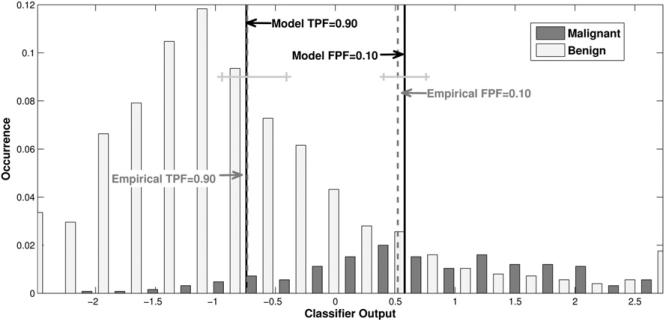
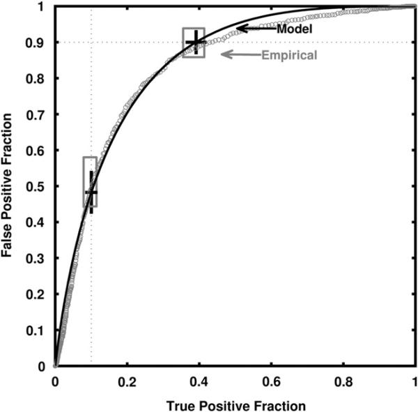
The real-data results of our leave-one-case-out analysis obtained for a linear discriminant analysis classifier of sonographic breast lesions are shown in Figures 7 and 8. AUC estimates of 0.84 ± 0.014 and 0.84 ± 0.013 were obtained directly from the empirical curves and by use of the proper binormal model, respectively. Figure 7 shows histograms of the output from the leave-one-out analysis for malignant and benign cases, together with the model-based and empirical output thresholds corresponding to TPF = 0.90 and FPF = 0.10. The model-based estimate of the threshold corresponding to TPF = 0.90 is t_TPF=0.90 = –0.74, whereas the empirical threshold is -0.72 with confidence interval (–0.946, –0.407). The model-based estimate of the threshold corresponding to FPF = 0.10 is t_FPF=0.10 = 0.58, whereas the empirical threshold is 0.55 with CI (0.403, 0.757). Figure 8 shows the corresponding model-based and empirical ROC curves, together with the operating points for each curve that correspond to the model thresholds t_TPF=0.90 and t_FPF=0.10. Although the empirical and model-based estimates lie well within each other's uncertainties, they provide confidence intervals that are somewhat different though largely overlapping.

Figure 7.

Output of the automated classifier for benign and malignant cases in ultrasonography, with both model-based and empirical estimates of the thresholds corresponding to true-positive fraction = 0.90 and false-positive fraction = 0.10. Also shown are 95% confidence intervals for the empirical estimates of threshold.

Figure 8.

The classifier's model-based-fit and empirical receiver operating characteristic curves together with model-based and empirical 95% confidence intervals for true-positive fraction (TPF) and false-positive fraction (FPF) at thresholds corresponding to a model-based TPF = 0.90 or a model-based FPF = 0.10. One should note that sampling errors are larger near “the center” of the ROC curve due to the sampling properties of proportions, because FPF and TPF are proportions; hence, larger residuals from receiver operating characteristic curve-fitting algorithms must be expected there.

DISCUSSION

This article has proposed and described the implementation of an approach for estimation of the relationship between test-result values and various case-specific quantities associated with the corresponding ROC curve estimate. That theory-based approach provides a principled alternative to the strictly ad-hoc method employed by our ROCKIT software (http://rocweb.bsd.uchicago.edu/MetzROC) in determining the relationship between various cutoff settings and ROC operating points, and it provides for the first time an ability to estimate the quantitative relationship between individual patients’ test-result values and the corresponding likelihood ratios. Simulation studies have shown that the approach provides little bias and acceptable standard errors when applied to data derived from the proper binormal model, whereas analysis of data acquired in an evaluation of computer diagnosis of breast lesions by ultrasonography indicated that our method's results are at least reasonable when applied to real data. The method is not computationally demanding, because for the most part it employs quantities already estimated by our semi-parametric PROPROC algorithm, and our experience to date has shown it to be reliable. Although we employed the proper binormal model, which we have found to be reliable and efficient (11), in principle the approach can be used with any “proper” ROC curve-fitting model, though its precision may differ with other such models.

The slope at any point on any ROC curve corresponds to the likelihood ratio associated with the corresponding test-result value; therefore, all convex ROC curves are necessarily “proper,” both in the sense that position on the curve is related monotonically to likelihood ratio and in the sense that the decision variable employed by the diagnostic test must have some monotonic relationship with likelihood ratio. Estimation of the latter relationship provides a basis for adjusting automated classifiers’ probability of malignancy outputs to account for different disease prevalences (29), for relating the results of various radiologists and/or automated classifiers that report their results on different scales (30) and for quantifying the extent to which classification of individual patients is “easy” or “difficult” for the diagnostic test in question.

When using the method described in this article, it is important to have good reason to expect that the ROC curve model upon which the method is based in fact describes the relevant data. This dictum is illustrated by the fact that although our simulation studies based on the proper binormal model showed the model-based estimates to agree acceptably with bootstrap estimates, the discrepancies found with our real data, though not statistically significant, were too great simply to be dismissed out of hand. The possibility of such differences usually is of less concern when computing model-based estimates of AUC, for example, because areas tend to depend less sensitively on local curve-shape restrictions imposed by particular ROC curve-fitting models. In particular, use of the proposed method for LLR estimation near FPF = 0 or near TPF = 1 must be approached with caution, because our simulation studies showed coverage of the CIs for LLR to be anticonservative, especially for high-skew ROC curves.

Formulation of simple guidelines regarding the curve shapes and ranges of likelihood ratio for which our algorithm is clearly appropriate or inappropriate lies beyond the scope of this article. To ensure that the method's estimates are reliable in a given application, we generally recommend that users of our software run a set of simulations like the ones described previously while using population parameter values similar to those estimated from the dataset in question and a particular trial design of interest (eg, the relevant numbers of actually positive and actually negative cases).

Finally, we note that the LLR, TPF, and FPF estimates obtained from Equations 5 and 7 must depend on prevalence, because according to Equation 4b, the medians of x are calculated from a mixture distribution associated with n_0,i actually negative cases and n_1,i actually positive cases, respectively. However, results obtained from truth-conditional medians, which are beyond the scope of this article, would not depend on prevalence, at least in the same way. We note also that the values of LR, LLR, TPF, and FPF associated with any particular case are not inherent characteristic of that case, but instead depend on the relative ease or difficulty with which a particular case can be distinguished from the population of cases having the opposite state of truth. Hence, the values of LR, LLR, TPF, and FPF associated with any particular case can serve as quantitative measures of case difficulty.

Software that implements the estimation procedure discussed in this article is available without charge from our website (http://rocweb.bsd.uchicago.edu/MetzROC).

REFERENCES

- 1.Wagner RF, Metz CE, Campbell G. Assessment of medical imaging systems and computer aids: a tutorial review. Acad Radiol. 2007;14:723–748. doi: 10.1016/j.acra.2007.03.001. [DOI] [PubMed] [Google Scholar]
- 2.Pepe MS. The statistical evaluation of medical tests for classification and prediction. Oxford University Press; Oxford; New York: 2004. [Google Scholar]
- 3.Zhou X-H, Obuchowski NA, McClish DK. Statistical methods in diagnostic medicine. Wiley-Interscience; New York: 2002. [Google Scholar]
- 4.Diabetes. World Health Organization; [July 14, 2010]. Available from http://www.who.int/topics/diabetes_mellitus/en/ [Google Scholar]
- 5.American College of Radiology . Breast imaging reporting and data system (BI-RADS) American College of Radiology; Reston, VA: 2003. [Google Scholar]
- 6.Kvam PH, Vidakovic B. Nonparametric statistics with applications to science and engineering. Wiley-Interscience; Hoboken, NJ: 2007. [Google Scholar]
- 7.Hanley JA. Receiver operating characteristic (ROC) methodology: the state of the art. Crit Rev Diagn Imaging. 1989;29:307–335. [PubMed] [Google Scholar]
- 8.Swets JA. Form of empirical ROCs in discrimination and diagnostic tasks: implications for theory and measurement of performance. Psychol Bull. 1986;99:181–198. [PubMed] [Google Scholar]
- 9.Swets JA. Indices of discrimination or diagnostic accuracy: their ROCs and implied models. Psychol Bull. 1986;99:100–117. [PubMed] [Google Scholar]
- 10.Hanley JA. The robustness of the “binormal” assumptions used in fitting ROC curves. Med Decis Making. 1988;8:197–203. doi: 10.1177/0272989X8800800308. [DOI] [PubMed] [Google Scholar]
- 11.Pesce LL, Metz CE. Reliable and computationally efficient maximum-likelihood estimation of “proper” binormal ROC curves. Acad Radiol. 2007;14:814–829. doi: 10.1016/j.acra.2007.03.012. [DOI] [PMC free article] [PubMed] [Google Scholar]
- 12.Metz CE, Herman BA, Shen JH. Maximum likelihood estimation of receiver operating characteristic (ROC) curves from continuously-distributed data. Stat Med. 1998;17:1033–1053. doi: 10.1002/(sici)1097-0258(19980515)17:9<1033::aid-sim784>3.0.co;2-z. [DOI] [PubMed] [Google Scholar]
- 13.Dorfman DD, Alf E. Maximum-likelihood estimation of parameters of signal-detection theory and determination of confidence intervals—rating method data. J Math Psychol. 1969;6:487–496. [Google Scholar]
- 14.Metz CE. Basic principles of ROC analysis. Semin Nucl Med. 1978;8:283–298. doi: 10.1016/s0001-2998(78)80014-2. [DOI] [PubMed] [Google Scholar]
- 15.Agresti A. Categorical data analysis. 2nd ed. Wiley-Inter-science; New York: 2002. [Google Scholar]
- 16.Wagner RF, Beiden SV, Metz CE. Continuous versus categorical data for ROC analysis: some quantitative considerations. Acad Radiol. 2001;8:328–334. doi: 10.1016/S1076-6332(03)80502-0. [DOI] [PubMed] [Google Scholar]
- 17.Yousef WA, Kundu S, Wagner RF. Nonparametric estimation of the threshold at an operating point on the ROC curve. Comput Stat Data Anal. 2009;53:4370–4383. [Google Scholar]
- 18.Drukker K, Pesce L, Giger M. Repeatability in computer-aided diagnosis: application to breast cancer diagnosis on sonography. Med Phys. 2010;37:2659–2669. doi: 10.1118/1.3427409. [DOI] [PMC free article] [PubMed] [Google Scholar]
- 19.Fleiss JL, Levin BA, Paik MC. Statistical methods for rates and proportions. 3rd ed. Wiley; Hoboken, NJ: 2003. [Google Scholar]
- 20.Ogilvie J, Creelman CD. Maximum likelihood estimation of receiver operating characteristic curve parameters. J Math Psychol. 1968;5:377–391. [Google Scholar]
- 21.Papoulis A. Probability, random variables, and stochastic processes. 2nd ed. McGraw-Hill; New York: 1984. [Google Scholar]
- 22.Kendall MG, Stuart A, Ord JK, et al. Kendall's advanced theory of statistics. 6th ed. Edward Arnold; Halsted Press; London, New York: 1994. [Google Scholar]
- 23.Metz CE, Pan X. “Proper” binormal ROC curves: theory and maximum-likelihood estimation. J Math Psychol. 1999;43:1–33. doi: 10.1006/jmps.1998.1218. [DOI] [PubMed] [Google Scholar]
- 24.Horsch K, Giger ML, Venta LA, et al. Automatic segmentation of breast lesions on ultrasound. Med Phys. 2001;28:1652–1659. doi: 10.1118/1.1386426. [DOI] [PubMed] [Google Scholar]
- 25.Horsch K, Giger ML, Venta LA, et al. Computerized diagnosis of breast lesions on ultrasound. Med Phys. 2002;29:157–164. doi: 10.1118/1.1429239. [DOI] [PubMed] [Google Scholar]
- 26.Drukker K, Giger ML, Vyborny CJ, et al. Computerized detection and classification of cancer on breast ultrasound. Acad Radiol. 2004;11:526–535. doi: 10.1016/S1076-6332(03)00723-2. [DOI] [PubMed] [Google Scholar]
- 27.Drukker K, Giger ML, Metz CE. Robustness of computerized lesion detection and classification scheme across different breast US platforms. Radiology. 2005;237:834–840. doi: 10.1148/radiol.2373041418. [DOI] [PubMed] [Google Scholar]
- 28.Efron B, Tibshirani R. An introduction to the bootstrap. Chapman & Hall; New York: 1993. [Google Scholar]
- 29.Horsch K, Giger ML, Metz CE. Prevalence scaling: applications to an intelligent workstation for the diagnosis of breast cancer. Acad Radiol. 2008;15:1446–1457. doi: 10.1016/j.acra.2008.04.022. [DOI] [PMC free article] [PubMed] [Google Scholar]
- 30.Horsch K, Pesce LL, Giger ML, et al. A scaling transformation for classifier output based on likelihood ratio: applications to a CAD workstation for diagnosis of breast cancer. Med Phys. 2012;39:2787–2804. doi: 10.1118/1.3700168. [DOI] [PMC free article] [PubMed] [Google Scholar]