

Abstract
The tertiary structures of protein complexes provide a crucial insight about the molecular mechanisms that regulate their functions and assembly. However, solving protein complex structures by experimental methods is often more difficult than single protein structures. Here, we have developed a novel computational multiple protein docking algorithm, Multi-LZerD, that builds models of multimeric complexes by effectively reusing pairwise docking predictions of component proteins. A genetic algorithm is applied to explore the conformational space followed by a structure refinement procedure. Benchmark on eleven hetero-multimeric complexes resulted in near native conformations for all but one of them (a root mean square deviation smaller than 2.5Å). We also show that our method copes with unbound docking cases well, outperforming the methodology that can be directly compared to our approach. Multi-LZerD was able to predict near native structures for multimeric complexes of various topologies.
Keywords: multimeric protein docking, protein structure prediction, 3D Zernike descriptors, genetic algorithm, protein-protein interaction
Introduction
Protein complexes are involved in many biological processes, mediating diverse functions that include transport, signal transduction, and gene regulation. Experimental evidence shows that not only binary complexes but also multimeric complexes play crucial roles in such functions. The importance and the abundance of protein interactions and complexes have been recently further highlighted by large-scale protein-protein interaction maps, electron microscopy, and electron tomography data of cells1–3. Structure information of the complexes provides a crucial insight about the mechanisms that regulate their functions and assembly. However, solving multimeric protein complex structures by experimental methods, such as X-ray crystallography, is often found to be more difficult than the structure of single protein chains. Thus, the development of computational protein docking prediction methods of multimeric complexes is extremely important and beneficial to the biology community.
In the past years, many protein docking methods have been developed as evidenced by the growing number of participants in the Critical Assessment of Prediction of Interactions (CAPRI)4. However, the majority of methods have focused on the assembly of two protein structures, also known as pairwise docking5–13. Despite the abundance14 and biological importance of multimeric protein complexes, surprisingly, only a handful of methods have been developed for multimeric protein complex prediction. Moreover, all of them except for CombDock15 limit their application to specific types of complexes, for example, homomeric and/or symmetric complexes16–18 or they require additional data to restrict the conformation search space19.
In this study we present a novel multiple protein docking algorithm, Multi-LZerD. It adopts a multi-stage approach, where the first stage performs a coarse-grained conformation search of pairwise docking candidates, followed by a combination of pairwise solutions using a genetic algorithm (GA). The conformation space is not limited to symmetric conformations, unlike most of the other methods. Generated multimeric complex structures are evaluated using an atomic detailed physics-based scoring function. Finally, structure refinement is applied to the resulting complex structures.
For the initial stage of pairwise docking, the procedure uses LZerD, which was developed previously by our group20. LZerD uses the 3D Zernike descriptor (3DZD), a mathematical rotational invariant surface shape representation. The 3DZD was shown to be effective at identifying complementary surface shapes from two proteins as docking interface regions. Although Multi-LZerD is based on pairwise docking predictions of all pairs of component proteins, it can also handle protein complexes where some pairs are not in contact with each other. This is made possible by representing a protein complex conformation using a spanning tree structure, where each protein (node) is only required to be connected to one of the other component proteins by an edge. The GA is designed to rearrange the tree structure by switching edges and reconnecting nodes.
Multi-LZerD is able to find near-native conformations for multimeric protein complexes of different docking topologies. It handles a considerably large number of pairwise combinations and is able to combine low-ranked pairwise predictions to obtain the correct multiple docking structures.
In the following sections we will provide a detailed description of each stage in the pipeline coordinated by Multi-LZerD. Then, we will describe the multiple docking results as well as further improvements that can be added to the methodology. The programs in Multi-LZerD and the datasets used are made available for academic users at our lab website, http://kiharalab.org/proteindocking.
Materials and Methods
Multi-LZerD provides a generic procedure for multiple protein docking that does not rely on the prior availability of biological information (e.g. symmetry or interaction sites). A general procedure can serve as a versatile basis that can incorporate additional stages to utilize more sources of information. The Multi-LZerD algorithm is overviewed in Figure 1. Given a set of protein structures which are known to form a complex, the first step employs a pairwise protein docking program, LZerD, to create a large number of docking conformations (decoys) for each pair of proteins. Note that we also compute docking decoys for pairs that may not actually interact in the complex, since we do not know beforehand the pairs that interact and the ones that do not. In Figure 1A, an example of a complex with four chains (A to D) is shown. Pairwise decoys are clustered to reduce redundant conformations.
Figure 1.

The Multi-LZerD Algorithm. A, Overview of the algorithm. The process is divided into 3 sections: generation of pairwise docking predictions using LZerD, construction of candidate multimeric structures progressively improved using a genetic algorithm and a refinement stage based on Monte Carlo optimization. B, GA operations performed to modify existing complexes. Mutation (panels B1, B2, B3) consists of randomly selecting an edge for removal followed by a random selection of another edge and prediction that allows the graph to be connected again. Crossover (B4, B5) follows a similar procedure, but it can only reconnect the graph using the edges in the parents. The number on each edge (arrow) specifies a pairwise docking decoy of the two connected chains.
Using the pairwise decoys as building blocks, a population of whole complexes is constructed. These initial full complex decoys are subject to iterative recombination and modification by a Genetic Algorithm (GA)21. A physics-based scoring function is used after each iteration to assess the quality of multimeric decoy structures. Lastly, after a number of iterations, the final set of decoys is clustered and representative complex structures are refined. Detailed descriptions of each stage are given in the subsequent sections.
LZerD: Local 3D Zernike descriptor-based pairwise docking program
Pairwise docking decoys are constructed using LZerD20. Candidate poses are sought for two input protein structures by applying geometric hashing22. LZerD uses the 3D Zernike descriptors (3DZDs), a rotational invariant mathematical surface representation of proteins23,24, to capture the shape complementarity of protein docking interfaces. To compute the 3DZD, a 3D grid function, f(x), that represents a local protein surface, is expanded into a series, in terms of Zernike-Canterakis basis25:
| (1) |
where −l<m<l, 0≤l≤n, and (n-l) even. , are the spherical harmonics and Rnl(r) are radial functions defined by Canterakis, constructed so that can be converted to polynomials, , in Cartesian coordinates. Now 3D Zernike moments of f(x) are defined by the expansion in this orthonormal basis, i.e. by the formula
| (2) |
The rotational invariance is obtained by defining the 3DZD series Fnl, as norms of vectors Ωnl:
| (3) |
The parameter n is called the order of 3DZD, which determines the resolution of the descriptor. An order of n = 10 is used for docking. Thus, surface shape is represented as a vector of coefficients in the series expansion.
The shape complementarity of two surface regions is quantified with the correlation coefficient of the vectors. Besides the shape complementarity term, we use a term for evaluating the direction of surfaces by using normals, a term for the interface surface area and a term for atom clashes (penalty term), all of which are combined linearly to rank docking poses (this score is later referred to as the shape-based score). LZerD is a geometric shape-based docking program; however, it can handle a certain degree of protein flexibility due to the controllable resolution of protein surface representation by the 3DZD. For each pair of component proteins 54,000 docking decoys are generated.
LZerD provides possible docking arrangements of two chains. It can be thought of as a shape-based screening process which will be later complemented by a more rigorous evaluation of multimeric conformations using a physics-based score.
Clustering decoy structures
The pairwise docking decoys for each pair of chains are clustered based on the root mean square deviation (RMSD) of Cα atoms. The procedure implemented is based on the clustering ideas conceived in ClusPro26. Two complexes are considered to be neighbors if they are closer than a threshold value (5.0 Å and 10.0 Å in our experiments). Once the clusters are created, the decoy with the best shape-based score is selected out of each cluster as a representative structure. The other members in the clusters will be deleted. The process typically reduces the number of pairwise predictions to around 15,000 to 20,000 representative decoys.
Conformation search using a genetic algorithm
The conformation space of a whole protein complex structure is explored by altering combinations of pairwise docking decoys. A whole complex conformation is represented by a spanning tree where a node denotes a component protein chain and an edge between two nodes specifies one of the pre-computed decoys of the two proteins that defines the relative conformation between the two. A spanning tree requires that each node is connected to at least another node by an edge and thus can define a single conformation of the whole complex. We found that the spanning tree representation is very suitable for constructing a multiple docking complex from pairwise decoys because not all pairs of nodes need to be connected. Since an edge is only used to express relative transformations between a subunit pair, the tree representation allows us to reconstruct different types of topological arrangements (e.g. fully connected, linearly connected complexes).
Multi-LZerD applies a GA to the population of spanning trees, each of which defines a different whole complex conformation27. A stochastic search strategy is chosen because finding a maximum scoring tree has been shown to be NP-Hard15. To start the process, the program creates an initial population of M randomly generated spanning trees. M is set to 200 in this work. These are subject to the application of two GA operations, mutation and crossover (Figure 1B). Mutation deletes one of the spanning tree edges and then selects a new edge randomly to reconnect the graph. It is possible that the same edge is selected again. For a newly selected edge, one of the pairwise docking decoys for the two proteins is randomly selected. The rest of the edges remain unaltered (Fig. 1B1, 1B2, 1B3). Crossover takes two candidate structures and creates a new individual by combining edges from the two parents (Fig. 1B4, 1B5). It will first create an empty graph and randomly select edges from the parents until a spanning tree is created. For each generation of the GA, 2M (i.e. 400) operations are performed.
At this point, Multi-LZerD computes two values for each new candidate: the number of clashes between atoms (atoms closer than 3.0 Å to other atoms) and the fitness score evaluated by the physics-based score (next section). A candidate complex structure is discarded if the number of clashing atom pairs exceeds a threshold value. Different thresholds were tested during our experiments that range between 200 and 600 clashing atoms. Subsequently, the remaining new individuals are mixed with the previous population, which are subject to clustering using the procedure described in the previous section. Only the top M ranked individuals by the physics-based score are kept. In case the clustering procedure reduces the population to less than M, randomly selected structures are added to complete the population for the next generation. The process is repeated for 3,000 iterations and the last M candidates will be subject to the refinement stage.
Physics-based score
LZerD uses a shape-based scoring scheme for ranking pairwise docking decoys. In contrast, whole multimeric protein complexes generated by the GA are evaluated and ranked with a physics-based scoring function. The function linearly combines the following terms: van der Waals, where repulsive and attractive parts of the term are considered separately12; an electrostatics term, which considers repulsive/attractive and short-range/long-range contributions separately28; a hydrogen and disulfide bond term29; two solvation terms30,31; and a knowledge-based atom contact term32. Weighting factors for the linear combination of the terms were trained on two datasets, the ZDOCK benchmark 2.033,34, which contains 84 pairwise unbound-unbound and bound-unbound docking structures, and also on 851 protein-protein dimeric complexes used by Huang and Zou to train their scoring function35. The combination of weight values was determined by logistic regression, where docking decoys with an interface RMSD of 2.5 Å or less were classified as correct predictions.
Structure refinement and final selection
The final population is clustered an additional time using a threshold value of 10.0 Å. As the last step in Multi-LZerD, each of the complex structures in the final population is subject to a structure refinement procedure. The procedure employs a Monte Carlo energy minimization with the Metropolis criterion, which randomly chooses one of the chains and applies a small perturbation of rotations and translations. A translation is a move of up to 0.1 Å to each of the three directions and a rotation is up to 0.05 radians to each of the three angles in a single step. The perturbation is tried 2,000 times.
Comparison to related methods
The first phase in Multi-LZerD shares similarities with CombDock15 since it is also based on the combination of pairwise docking predictions using a shape-based score. They both try to search the combinatorial space, however, the search procedure used by both methods is significantly different. The approach adopted by CombDock relies on the greedy selection of spanning trees to reduce the number of conformations explored. On the other hand, Multi-LZerD uses a stochastic approach to pursue incremental optimization of candidate structures.
Additionally, the scoring method differs between them because Multi-LZerD employs a more rigorous physics-based scoring during the combinatorial search. Also it uses the 3DZD, which allows a certain level of soft-docking through the shape-based score. In contrast, CombDock uses a single non-polar buried surface area term combined with the other solely shape-based criteria. In the results section we demonstrate that these differences allow Multi-LZerD to perform considerably better in unbound docking scenarios.
HADDOCK is another multimeric docking method19. The main difference between Multi-LZerD and HADDOCK is that the latter is an information-driven approach that requires the specification of interaction sites as constraints, which can be either experimental or predicted information. We could not use HADDOCK for comparison with Multi-LZerD because it did not run without additional interaction site information or by specifying all the surface residues as potential docking interface residues. Saladin et al. also created an open source molecular docking library, PTOOLS36. The authors provided an example of their library usage for three protein docking. However, since it was shown as an example of combining source code in the library, they are not integrated for multiple docking and thus the protein complex structure can be constructed only when correct docking poses are known beforehand.
Availability of the software and the datasets
The Multi-LZerD program is made freely available for the academic community at our lab website, http://kiharalab.org/proteindocking. In addition, the docking program, LZerD, which is the base of PI-LZerD, is also made available at http://kiharalab.org/proteindocking. Our benchmarks were executed on a Linux machine running Ubuntu 10.04, kernel version 2.6.32–31, with an Intel i7 processor at 2.67GHz, with 12 GB of main memory. The execution time for LZerD is, on average, 3 to 4.5 hours to generate pairwise docking predictions. Once pairwise docking predictions are prepared, the running time for Multi-LZerD, is 30 seconds to a minute per generation. In addition to the programs, the datasets used in this study are also made available at the same web site.
Results
We have benchmarked Multi-LZerD on eleven multimeric complexes taken from the 3D Complex database14 (Table 1). This set includes complexes with three, four, and six chains, which have a variety of topologies (the pattern of interacting chains). According to the 3D Complex database, interacting chains are defined as those that have at least ten contacting residues, where a residue pair is defined as in contact if an atom pair is closer than the sum of their van der Waals radii plus 0.5 Å. Both bound and unbound cases have been tested in order to examine Multi-LZerD’s ability to identify correct complexes in the vast conformation space and also the possibility to manage conformational change, which is present in typical unbound docking scenarios. The following sections will show different analyses that were performed in order to assess the validity of our approach as well as its performance compared to existing methods.
Table 1.
Dataset used to evaluate Multi-LZerD.
| PDB | Chains | Length1 | Topology |
|---|---|---|---|
| 2AZE | 3 | 307 | 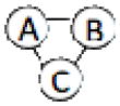 |
| 1A0R | 3 | 650 | |
| 1VCB | 3 | 390 | |
| 1K6N | 3 | 855 | 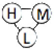 |
| 1B9X | 3 | 654 | |
| 6RLX | 4 | 104 | |
| 1QGW | 4 | 497 | 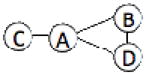 |
| 1LOG | 4 | 466 | 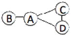 |
| 1NNU | 4 | 578 | 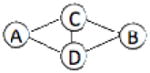 |
| 1RHM | 4 | 498 | 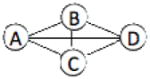 |
| 1I3O | 6 | 812 | 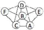 |
Total length of the chains according to the 3D Complex Database.
Shape-based and physics-based scoring functions
Our pairwise docking program, LZerD, uses a scoring function that is mainly based on shape-based components (e.g. shape complementarity). In this work we extended the scoring function to incorporate more rigorous physics-based scoring components that, while considerably more expensive to compute, can provide a higher accuracy. Our first task was to compare these two types of scoring schemes in terms of their performance at identifying near native docking structures. Figure 2 shows examples of ranking results for pairwise docking decoys between two interacting protein chains, A–C and B–D in 1NNU, by the two scores. There are 54,000 decoys for each case, which were computed by LZerD. The same decoy sets were ranked using the two scores and then the number of near native structures (RMSD ≤ 4Å) (y-axis) within certain ranks (x-axis) were calculated.
Figure 2.

Performance comparison between the shape-based score and the physics-based score. Rankings are shown for pairwise docking predictions using subunits in 1NNU. Panel A shows results for chains A and C while panel B shows scores chains B and D. Predictions with an RMSD of 4.0 Å or lower were counted as hits.
In both cases, the physics-based score clearly outperforms the shape-based score. In the case of the decoys of A and C chains, the physics-based score ranked almost two times (129 vs. 62) more near native decoys than the shape-based score within the top 1,000 ranks. As for the chain pair of B and D, the physics-based score obtained 101 near native decoys within top 1,000 while the shape-based score obtained 40 hits. Since it is clear that the physics-based score is superior to the shape-based score at identifying near native structures, we used the former for ranking multimeric complex structures in the conformation search stage by GA. The shape-based score is still used in the pairwise docking stage (LZerD), since the aim of the initial stage is to provide candidate structures for the later Genetic Algorithm search and does not need more time consuming scoring and ranking.
Docking performance
Table 2 shows the summary of the predictions by Multi-LZerD on the eleven multimeric protein complexes. The global Cα RMSD and the fnat value of the best model in the last generation of the GA as well as the RMSD of the model after the refinement are shown. The fnat is the fraction of native residue-residue contacts in a predicted conformation, where atoms are considered to be in contact when they locate closer than 5.0 Å to each other37. The GA optimization was performed for 3,000 generations with a population size of 200. The structures of the refined models are superimposed on the native structures in Figure 3.
Table 2.
Summary of the bound docking prediction results.
| PDB ID | Multi-LZerD | Pairwise Ranks | Refinement | CombDock | ||||
|---|---|---|---|---|---|---|---|---|
| RMSD(Å)1 | Rank2 | RMSD(Å) | fnat | RMSD(Å)3 | Rank | |||
| 2AZE | 0.99 | 1 | A–B | 1 | 0.73 | 0.60 | 0.79 | 1 |
| A–C | 918 | |||||||
| 1A0R | 0.84 | 1 | B–G | 1 | 0.53 | 0.95 | 0.93 | 1 |
| B–P | 2 | |||||||
| 1VCB | 1.15 | 113 | A–B | 6 | 1.09 | 0.50 | 0.55 | 1 |
| B–C | 13 | |||||||
| 1K6N | 1.11 | 1 | H–L | 870 | 0.89 | 0.84 | 0.78 | 1 |
| H–M | 5077 | |||||||
| 1B9X | 0.63 | 1 | A–B | 13 | 0.45 | 0.50 | 0.66 | 1 |
| A–C | 74 | |||||||
| 6RLX | 4.49 | 171 | A–B | 118 | 4.39 | 0.12 | 7.37 | 7 |
| B–D | 293 | |||||||
| C–D | 24 | |||||||
| 1QGW | 3.23 | 4 | A–B | 526 | 1.50 | 0.19 | 0.87 | 1 |
| A–C | 14 | |||||||
| B–D | 3 | |||||||
| 1LOG | 1.90 | 63 | A–B | 2 | 1.59 | 0.45 | 1.73 | 2 |
| A–C | 25714 | |||||||
| C–D | 1 | |||||||
| 1NNU | 1.12 | 4 | A–C | 1 | 0.99 | 0.71 | 0.83 | 1 |
| B–D | 1 | |||||||
| C–D | 16 | |||||||
| 1RHM | 1.07 | 1 | A–B | 1 | 1.00 | 0.36 | 0.96 | 1 |
| B–D | 9 | |||||||
| C–D | 1 | |||||||
| 1I3O | 2.41 | 4 | A–B | 1 | 1.57 | 0.27 | 1.90 | 6 |
| B–D | 24 | |||||||
| B–E | 2304 | |||||||
| C–D | 2 | |||||||
| D–F | 3218 | |||||||
The best Global Cα RMSD to the native structure in the last GA generation.
The rank in terms of the physics-based score in the last GA generation.
The best Global Cα RMSD is shown.
Figure 3.

Visualization of native structures and best prediction obtained by Multi-LZerD. For each test case, chains are shown using different colors for native (blue, red, yellow, green, cyan, purple) and predicted (light blue, salmon, orange, light green, teal, pink).
A near native structure with an RMSD of less than 2.5Å was obtained for ten out of 11 test cases and the additional case was predicted at a RMSD of 4.39 Å. It is noteworthy that Multi-LZerD managed to generate good predictions for all the complexes with different topologies including the ones whose nodes (protein chains) are not fully connected, e.g. linearly connected complexes, such as 1A0R and 1VCB (Table 1). This indicates that the scoring scheme (the physics-based score) has successfully identified the correct topology with less interacting pairs among all the other conformations explored in the GA-based search. It is also encouraging to find that correct pairwise decoys were selected even from very low pairwise ranks, because they yield a good overall score as a whole complex when combined with the other pairwise decoys. For example, a correctly selected pairwise conformation for chains A and C in 2AZE was ranked at 918; and the conformation for the chains A–C in 1LOG was selected with a rank of 25,714. As an example, we further investigated the case of 2AZE. The 1st ranked decoy of A–B was present in the population starting at generation 20 in the GA optimization (albeit not with the A–C decoy at rank 918). The A–C decoy 918 was sampled once at generation 459, however, it was dropped from the subsequent population because it was not linked with the A–B decoy 1. Later, at generation 759 the A–C decoy 918 was sampled again along with the A–B decoy 1, yielding the prediction that ultimately becomes the best one found. This shows how a correct pairwise decoy ranked low can be identified when combined with the appropriate complement.
Turning our attention to the refinement, all the structures have improved by applying the refinement procedure. The range of the improvements is from 0.07 Å (1RHM) to 1.73 Å (1QGW). Importantly, the refinement has never deteriorated the input structures, which is not trivial in general in the protein structure prediction field38,39.
The results in Table 2 show that all the fnat values fall into the high or medium accuracy for the CAPRI protein interaction prediction criteria4. The fnat values of 1RHM, 1QGW, 6RLX and 1I3O are relatively lower than the others. The fnat is sensitive to the structure details and can quickly deteriorate by slight changes of docking orientation. This is especially true for multiple docking cases (see also the predicted structures in Figure 3; they all look reasonably fine). The fnat could be improved by applying a more delicate structure refinement procedure, for example, one that uses a physics-based scoring function specifically optimized to be sensitive to subtle changes in conformation. These are left as future work.
We have also compared our results against predictions generated by CombDock, since it is the only multiple docking method that can be directly compared to our approach (Table 2). Comparing the RMSD values, Multi-LZerD and CombDock perform similarly well in the ten cases for which Multi-LZerD finds a near-native prediction. Also, our approach manages to get a considerably better result for the more challenging 6RLX case. In terms of the score rank of the hits, CombDock had more near native predictions (within 2.5Å RMSD) at the first rank.
Although improvement by Multi-LZerD by CombDock was not observed in the bound cases, our method shows significantly better performance in the unbound docking cases (Table 3). Unbound docking benchmark studies, in general, use monomer conformations solved in an isolated state to simulate most of the actual blind docking situations. Unbound docking predictions are more difficult than bound docking predictions due to conformational change of monomer structures between their bound and unbound form. For all the chains in the bound dataset, we searched unbound monomer conformation in the PDB, but none of them were available. Therefore, we performed homology modeling for the subunits of the complexes. Homologous protein structures for the tested proteins were searched by BLAST40 against the PDB and the structures were modeled by SWISS-MODEL server41,42. Out of the eleven complexes, we modeled six of them for which templates were available. The templates used are 2QNS, 3FB4, 1LQB, 3PD1, 1XF6, and 1LOA respectively, for modeling chains in 1A0R, 1NNU, 1VCB, 1RHM, 1QGW, and 1LOG. A detailed description of the structures used as templates is provided in Table 4. As shown in Table 4, the template structures used for modeling are in their bound form, however, they are in different crystal structures, complexed with different bound counterparts or the topologies of the template complexes are different from the targets. The RMSDs of resulting modeled chain structures and target chains range from 0.07 to 1.88 Å with an average of 0.876 Å. There are cases that the template is the same protein (i.e. 100% sequence identity) to the target chain, but the conformation of those templates is not closer to the targets (the average RMSD is 0.882 Å) as compared with the average RMSD of all the modeled subunits. In the case of 1A0R, 2QNS served as a good template for chains B and G but not for chain P because the length of 1A0RP and 2QNSC is very different (188 residues and 8 residues, respectively). Thus, chain P is kept in its bound form. Three different cases were created using the modeled chains, which are labeled 1A0Rbg, 1A0Rb, and 1A0Rg. The lower case suffixes indicate the chains whose structures are substituted by models. For example, 1A0Rbg indicates that chains B and G are homology models while chain P is kept in its bound form. For 1NNU, the A chain of 3F4B was used to model all four chains. 1NNU-A and 1NNU-B are identical and aligned at residue 8 to 235 of 3F4B-A, while chain C and D of 1NNU are aligned at residue 257–316 of 3F4B-A. A similar situation occurred with 1RHM where the two protein units are matched to distinct parts in 3PD1 chain A (1RHM-A and 1RHM-C aligned at the residue 1 to 147 of 3PD1-A, while the B and the D chain aligned at the residue 148 to 249. The unbound datasets are made available for download to use at http://kiharalab.org/proteindocking/. The same procedure that was applied to the bound cases was executed using these ten modeled cases (Table 3).
Table 3.
Summary of unbound docking results.
| PDB ID | Multi-LZerD | Pairwise Ranks | Refinement | CombDock | ||||
|---|---|---|---|---|---|---|---|---|
| RMSD(Å)1 | Rank2 | RMSD(Å) | fnat | RMSD(Å)3 | Rank | |||
| 1A0Rbg | 6.78 | 192 | B–G | 367 | 6.65 | 0.30 | 18.12 | 2 |
| B–P | 321 | |||||||
| 1A0Rb | 2.16 | 1 | B–G | 1 | 1.97 | 0.30 | 21.18 | 9 |
| B–P | 6679 | |||||||
| 1A0Rg | 1.40 | 1 | B–G | 2 | 1.17 | 0.48 | 8.38 | 4 |
| B–P | 4 | |||||||
| 1VCBabc | 1.11 | 1 | A–B | 22 | 1.09 | 0.42 | 1.39 | 1 |
| B–C | 23 | |||||||
| 1QGWabcd | 0.98 | 12 | A–B | 289 | 0.90 | 0.35 | 9.39 | 8 |
| A–C | 12 | |||||||
| B–D | 138 | |||||||
| 1NNUabcd | 1.73 | 2 | A–C | 5 | 1.00 | 0.21 | 16.76 | 31 |
| B–D | 1 | |||||||
| C–D | 156 | |||||||
| 1NNUab | 1.40 | 14 | A–C | 5 | 1.11 | 0.31 | 20.25 | 29 |
| B–D | 51 | |||||||
| C–D | 434 | |||||||
| 1NNUcd | 2.60 | 7 | A–C | 84 | 1.72 | 0.37 | 18.36 | 7 |
| B–D | 80 | |||||||
| C–D | 59 | |||||||
| 1LOGabcd | 1.79 | 34 | A–B | 9712 | 1.75 | 0.50 | 1.56 | 1 |
| A–C | 67 | |||||||
| C–D | 6229 | |||||||
| 1RHMabcd | 2.16 | 4 | A–B | 14 | 1.38 | 0.44 | 0.95 | 2 |
| B–D | 5 | |||||||
| C–D | 2 | |||||||
The best Global Cα RMSD to the native structure in the last GA generation.
The rank in terms of the physics-based score in the last GA generation.
The best Global Cα RMSD is shown.
Table 4.
Construction of structures for the unbound dataset.
| Bound Structure | Model | Model differences | ||||
|---|---|---|---|---|---|---|
| PDB | Chain | PDB | Chain | Topology | RMSD (Å)1 | Seq. Identity (%)2 |
| 1A0R | B | 2QNS | A | 1.25 | 99.7 | |
| G | B | 1.67 | 37.1 | |||
| 1VCB | A | 1LQB | A | 1.17 | 100.0 | |
| B | B | 1.20 | 100.0 | |||
| C | C | 1.32 | 100.0 | |||
| 1QGW | A | 1XF6 | A | 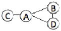 |
0.11 | 98.7 |
| B | B | 0.07 | 100.0 | |||
| C | C | 0.25 | 99.4 | |||
| D | D | 1.88 | 99.4 | |||
| 1NNU | A, B | 3F4B | A | 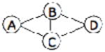 |
0.52 | 78.5 |
| C, D | A | 0.49 | 85.0 | |||
| 1LOG | A | 1LOA | A | 0.79 | 100.0 | |
| B | B | 0.72 | 100.0 | |||
| C | C | 0.82 | 100.0 | |||
| D | D | 0.78 | 100.0 | |||
| 1RHM | A, C | 3PD1 | A | 1.07 | 100.0 | |
| B, D | A | 0.78 | 99.1 | |||
RMSD between the bound structure and the model is reported.
The sequence identity between the template used for homology model and the target protein.
It is observed that Multi-LZerD was able to obtain a near native conformation for all but one case, 1A0Rbg. For the case of 1A0Rbg, despite a larger RMSD of 6.65Å obtained, the overall conformation is correct as indicated by a comparable fnat of 0.30 to the other predictions with a small RMSD. Table 3 also shows that the refinement step consistently makes improvements. In particular, models for 1NNUcd and 1NNUabcd are significantly refined by 0.88 Å and 0.73 Å RMSD, respectively. Moreover, it is shown that Multi-LZerD outperforms CombDock in eight cases among the ten unbound cases in terms of the RMSD of the predicted structures. In the two cases, 1LOGabcd and 1RHMabcd, for which CombDock achieves a lower RMSD, Multi-LZerD also produces near native structures (an RMSD of 1.75 Å and 1.38 Å, respectively) and the RMSD difference between Multi-LZerD and CombDock models is less than 0.5 Å. CombDock was able to find three near native structures, however, it produced decoys that are considerably far from the native structure for the rest of the seven cases. The superior performance of Multi-LZerD with respect to CombDock is consistent with our previous study of pairwise protein docking by LZerD. We showed in that paper that LZerD performs overwhelmingly better than PatchDock10, the base pairwise docking algorithm used in CombDock, in unbound docking cases, while they perform similarly on bound cases.
The main reason for Multi-LZerD’s better performance in unbound cases could be due to the more rigorous physics-based scoring function, compared to the score used by CombDock, and also because of the 3DZD used by Multi-LZerD, which is tolerant to a certain level of conformational change that occurs between unbound and bound structures.
Correlation between the RMSD and the physics-based score
The scoring function can select near native structures from a pool of generated decoys if it correlates well to the RMSD values of decoy structures. Here we examined the physics-based score and the RMSD of the 200-structure population in the final generation of the GA simulations. The cases for 2AZE, 1RHM, 1A0R, and 1NNU are shown in Figure 4 and the data for the rest of the complexes are shown in Figure S1 (Supplemental Material). A lower value is better in this scoring function. The population contains structures of various topologies, for example, structures of fully connected topology (where every pair of chains interact) exist in the population for 1A0R, which has a linear topology (Table 1).
Figure 4.

RMSD and physics-based scores in final GA generation. Each panel shows the relationship between the Cα RMSD and corresponding score after 3,000 GA optimization generations A, 2AZE; B, 1RHM, C, 1A0R, and D, 1NNU, respectively Additional plots are shown in Figure S1 for the rest of the test cases.
It can be seen that the scoring function clearly discriminates the correct (i.e. nearest to native) predictions as the lowest energy in the cases of 2AZE, 1A0R, and 1RHM. For the cases of 1NNU, the nearest native structure is found at the fourth rank (Table 2). Thus, the physics-based score performed reasonably well at identifying near native structures. It is worth noting that these plots correspond to the final 200 complexes in the GA optimization. This means that the scoring function was able to discard a considerable number of incorrect predictions up to the 3,000th generation. As a final remark, it may appear from the plots as if the sampling around the near-native structures is not sufficient, but this is an artifact of the clustering procedure that selects a representative for each cluster.
Genetic Algorithm optimization convergence
We also investigated how the GA converges towards a good prediction. Ideally, as the simulation progresses, it is expected that the score keeps lowering until convergence, which is associated with the quality improvement of the predicted structure (i.e. a lower RMSD).
Figure 5 shows the score and the RMSD for the best prediction (the lowest RMSD structure) at each GA generation in four docking predictions, 2AZE (panel A), 1RHM (B), 1A0R (C) and 1NNU (D). Additionally, data for the rest of the protein complexes in the dataset are provided in Figure S2. In all the cases, the lowest RMSD structure in the population reaches close to native in the GA optimization starting from the initial structures of 15–20Å RMSD. Furthermore, the close to native structures appear relatively quickly, e.g. within 100 generations in three cases and within 200 in two other cases. The decrease of the score and the RMSD occur concurrently in general, although there are situations where a decrease of the score did not associate with a drop of the RMSD value. This is due to the imperfect scoring function, as we have also observed in Figure 4 and Figure S1.
Figure 5.

The evolution of the score and the RMSD. Each panel shows the best RMSD prediction in the population at each step of the GA generation for A, 2AZE; B, 1RHM; C, 1A0R; and D, 1NNU, respectively. Although the maximum number of generations of GA was set to 3,000, the plots show up to a generation when it converges to a near-native solution. Plots for the rest of protein complexes in Table 1 are shown in Figure S2.
Finally, it is noticed that a sharp drop in the score and the RMSD occurs frequently in the plots. For example, in the case of 2AZE, no essential change was observed up to the 500th generation followed by a drastic improvement of the score and the RMSD. This may be due to the combinatorial nature of the multiple docking optimization; namely, fitting structure pieces of certain chain pairs triggers identification of correct compatible structures of the other pairs in an “allosteric” fashion.
Prediction accuracy of subcomplexes in decoys
In this section we further investigate if a subset of chains is correctly arranged in entire complexes. Even when the global RMSD of a whole predicted complex is not small, we observe quite often cases that a subcomplex within the whole complex is correctly predicted. Such predictions would also be useful in practice since, for example, interface residues are predicted correctly in the subcomplexes43.
In Figure 6 we show examples of the distribution of the number of decoys that contain subunits predicted within an RMSD of 4.0 Å (called subcomplex hits). For each decoy, we identified a subcomplex hit with the largest number of chains. Decoys in the final population generated by the GA optimization are separated into six bins according to the global RMSD to the native structure and subcomplex hits are counted for decoys in each bin. The total number of decoys shown in the four panels is different because they are clustered. Figure 6A shows the case of a three-chain complex, 1A0R. For this complex, we have one decoy that is correctly predicted within an RMSD of 4.0 Å (the left most bar in Fig. 6A). An interesting observation is that all the decoys including those that have a global RMSD of 20.0 Å or higher contain a correctly predicted two-chain subcomplex. Looking at the intermediate results in the GA optimization, we found that the B–G chain pair was correctly predicted earlier in the optimization while the correct relative orientation of the P-chain to the B–G pair was found in a later generation.
Figure 6.

Analysis of subcomplex prediction accuracy. Correctly predicted subcomplexes within the whole complex were analyzed. The final population for four cases 1A0R (panel A), 1NNU (B), 1QGW (C), and 1I3O (D) was classified according to their global RMSD into six bins. Each stacked bar shows the number of correctly predicted subcomplexes with an RMSD of 4.0 Å. The size (the number of chains) is the subcomplex hits are shown in the gray scale.
Figure 6B and 6C show results of four chain complexes, 1NNU and 1QGW, respectively. For both 1NNU and 1QGW, all the decoys contain at least a two-chain subcomplex hit. In the case of 1NNU, the B–D subcomplex was correctly predicted in 125 decoys (89.3%) in the final population and the A–C subcomplex was correctly predicted in all the decoys. There is one decoy with an RMSD of over 20 Å, yet it has a three-chain subunit within 4.0 A. Å similar behavior is shown for 1QGW. The B–D chain subcomplex was correctly predicted in all decoys while the A–C pair is correctly docked in 66.7% of the decoys. Finally, the results for 1I3O, a six-chain complex, is shown in Figure 6D. Remarkably, we found that up to five chains are correctly assembled in all except four decoys, and the rest of the four decoys have four chains that are assembled within 4.0 Å. For 1I3O, the problem was the chain F, which was misplaced in the majority of the decoys. Since the overall complex structure is large, misplacing a single chain can result in a large global RMSD.
In Figure 7, examples of decoys are shown that have a high overall RMSD yet contain a correct subcomplex of an RMSD of less than 4.0 Å. Figure 7A is a decoy of 1A0R (three-chain complex) with a global RMSD of 15.1 Å. Despite of the large RMSD, the relative orientations of chain B (green, native; blue, predicted) and G (yellow, native; red, predicted) are correctly predicted. Chain P is shown in gray. Figure 7B is a decoy of 21.7 Å global RMSD for 1NNU (four chain complex). In this decoy three chains, A, C, and D, are correctly assembled. Figure 7C is an example of decoy of 1QGW (four chain complex). Although its global RMSD to the native is 18.6 Å, chain B and D are correctly arranged. The last example (Figure 7D), is a decoy of a six-chain complex, 1I3O. A seemingly large RMSD of 14.17 Å comes from misarrangement of chain F, and the rest of the five chains are correctly assembled within 4.0 Å RMSD.
Figure 7.

Examples of decoys with correct subcomplex. The structure of decoys with a high global RMSD of the whole complex but present subcomplexes within 4.0 Å RMSD are shown. A, a decoy for 1A0R (3 chain complex) with a global RMSD of 23.59Å. Chains B and G are docked correctly. Green and blue show the native and predicted locations of Chain B, while yellow and red show native/predicted positions of Chain G. Chain P is shown in gray. B, a 1NNU decoy (four chains) with a global RMSD of 21.67Å. Three chains, A, C, and D, are docked correctly. The color code is the same as used in A. C, a 1QGW decoy (four chains) with a global RMSD of 18.61Å. The subcomplex of chain B and D are within 4.0 Å. D, a decoy predicted for 1I3O (six chains) with a global RMSD of 25.25 Å. Five chains out of six (except for F) are docked within 4.0 Å.
The analysis shows the majority of the decoys contain correctly predicted subcomplexes, even when their global RMSD shows a large value. The number of decoys with a correctly predicted subcomplex for the bound (Table 2) and the unbound (Table 3) docking experiments is summarized in Table SI (Supplemental material). In the bound docking dataset (Table SIA), remarkably, at least two chains were correctly assembled in all the decoys of all the target proteins except for 1VCB and 6RLX. In the case of unbound docking experiments (Table SIB), the majority of the decoys have at least a two-chain subcomplex hit. Even for 1A0Rbg (three-chain complex), whose best global RMSD ended up with 6.78 Å (Table 3), two chains were correctly docked in 10 % of the decoys.
Decoys with correct subcomplexes will be practically useful since interface residues of the subcomplexes are correctly identified. This observation also indicates the importance of examining subcomplexes in multiple docking predictions. Conventional measures, e.g. RMSD or fnat, are designed to evaluate the accuracy of single protein models or pairwise protein docking models. Thus, naively applying the measures to multiple docking results would miss the meaningful difference between partially correct decoys from the totally incorrect decoys.
Discussion
In this work, we have proposed a multi-layered approach for multimeric protein docking prediction, Multi-LZerD, which combines a coarse-grained pairwise pose search, a combinatorial complex conformation search, clustering, physics-based scoring, and structure refinement. Unlike almost all of the other existing methods, the application of Multi-LZerD is not restricted to symmetric multimers nor does it need extra information for limiting the conformation search space.
The benchmark results show that our approach has successfully obtained near-native structures for ten bound docking cases tested, with a single case with medium quality prediction, and all but one unbound case. By representing the protein complex conformation using a spanning tree, Multi-LZerD can assemble multimeric protein complexes of any topology from pairwise solutions. Remarkably, the approach could assemble correct structures even when some of the correct pairwise decoys are ranked very low in the decoy pool. Because the state-of-the-art pairwise protein docking methods are not yet able to consistently return a near-native structure within the top few ranks, considering a large number of pairwise predictions is essential for successful overall prediction. As noted before, the population size used in the GA was 200 per generation, which is a very small amount compared to the total combinatorial space. The mutation and the crossover operations on spanning trees were effective in exploring the vast conformation space. Furthermore, we observed that the majority of decoys with an apparent overall RMSD contain accurately predicted subcomplexes, which will be still useful for practical use.
The current version of Multi-LZerD can be enhanced in several directions. First, it is not difficult to implement options to take additional information, such as symmetry, interacting pairs, or interface residues, into account. Of course such information is not generally available, but it will reduce the conformation search space significantly in case it is available. Secondly, we are planning to implement a more thorough refinement procedure. The current refinement step was shown to improve an input complex structure constantly by up to 0.84 Å in the benchmark set. However, it is designed to make small improvements by perturbing the docking structure by a small distance and angle. More extensive refinement may be needed especially when the initial pool of pairwise decoys does not contain near native solutions. An idea is to perform several rounds of optimization of docking orientation of each individual chain, with respect to the rest of the complex structure, by detaching it from the complex and then re-docking them using the pairwise docking procedure. This is similar to an optimization approach for multiple sequence alignments implemented in one of the best multiple sequence alignment programs, MUSCLE44. Third, GA is suitable for parallel computing, thus fully taking advantage of high-performance computing should increase its execution-time performance.
Despite the fact that a significant number of hetero-oligomeric protein complexes are known to play important roles in a cell, multimeric protein-protein docking has been fairly unexplored yet. Computational protein docking needs to shift from classical pairwise to the multimeric realm, as experimental structural data and omics data has already shifted their focus.
Supplementary Material
Acknowledgments
This work was supported by the National Institute of General Medical Sciences of the National Institutes of Health (R01GM075004, R01GM097528) and the National Science Foundation (DMS0800568, EF0850009, IIS0915801). JER is a Fulbright Science and Technology Fellow.
References
- 1.Bárcena M, Koster AJ. Electron tomography in life science. Seminars in Cell & Developmental Biology. 2009;20:920–30. doi: 10.1016/j.semcdb.2009.07.008. [DOI] [PMC free article] [PubMed] [Google Scholar]
- 2.Levy ED, Pereira-Leal JB. Evolution and dynamics of protein interactions and networks. Curr Opin Struct Biol. 2008;18:349–57. doi: 10.1016/j.sbi.2008.03.003. [DOI] [PubMed] [Google Scholar]
- 3.Zhou ZH. Towards atomic resolution structural determination by single-particle cryo-electron microscopy. Current Opinion in Structural Biology. 2008;18:218–28. doi: 10.1016/j.sbi.2008.03.004. [DOI] [PMC free article] [PubMed] [Google Scholar]
- 4.Janin J. Protein-protein docking tested in blind predictions: the CAPRI experiment. Molecular BioSystems. 2010;6:2351–62. doi: 10.1039/c005060c. [DOI] [PubMed] [Google Scholar]
- 5.Ben-Zeev E, Eisenstein M. Weighted geometric docking: incorporating external information in the rotation-translation scan. Proteins. 2003;52:24–7. doi: 10.1002/prot.10391. [DOI] [PubMed] [Google Scholar]
- 6.Tovchigrechko A, Vakser IA. GRAMM-X public web server for protein-protein docking. Nucleic Acids Research. 2006;34:W310–4. doi: 10.1093/nar/gkl206. [DOI] [PMC free article] [PubMed] [Google Scholar]
- 7.Pierce B, Weng Z. ZRANK: reranking protein docking predictions with an optimized energy function. Proteins. 2007;67:1078–86. doi: 10.1002/prot.21373. [DOI] [PubMed] [Google Scholar]
- 8.Chen R, Li L, Weng Z. ZDOCK: an initial-stage protein-docking algorithm. Proteins. 2003;52:80–7. doi: 10.1002/prot.10389. [DOI] [PubMed] [Google Scholar]
- 9.Dominguez C, Boelens R, Bonvin AMJJ. HADDOCK: a protein-protein docking approach based on biochemical or biophysical information. J Am Chem Soc. 2003;125:1731–7. doi: 10.1021/ja026939x. [DOI] [PubMed] [Google Scholar]
- 10.Schneidman-Duhovny D, Inbar Y, Nussinov R, Wolfson HJ. PatchDock and SymmDock: servers for rigid and symmetric docking. Nucleic Acids Research. 2005;33:W363–7. doi: 10.1093/nar/gki481. [DOI] [PMC free article] [PubMed] [Google Scholar]
- 11.Moreira IS, Fernandes PA, Ramos MJ. Protein-protein docking dealing with the unknown. Journal of Computational Chemistry. 2010;31:317–42. doi: 10.1002/jcc.21276. [DOI] [PubMed] [Google Scholar]
- 12.Gray JJ, et al. Protein-protein docking with simultaneous optimization of rigid-body displacement and side-chain conformations. Journal of Molecular Biology. 2003;331:281–99. doi: 10.1016/s0022-2836(03)00670-3. [DOI] [PubMed] [Google Scholar]
- 13.Ritchie DW. Recent progress and future directions in protein-protein docking. Current Protein & Peptide Science. 2008;9:1–15. doi: 10.2174/138920308783565741. [DOI] [PubMed] [Google Scholar]
- 14.Levy ED, Pereira-Leal JB, Chothia C, Teichmann SA. 3D complex: a structural classification of protein complexes. PLoS Computational Biology. 2006;2:e155. doi: 10.1371/journal.pcbi.0020155. [DOI] [PMC free article] [PubMed] [Google Scholar]
- 15.Inbar Y, Benyamini H, Nussinov R, Wolfson HJ. Prediction of multimolecular assemblies by multiple docking. J Mol Biol. 2005;349:435–47. doi: 10.1016/j.jmb.2005.03.039. [DOI] [PubMed] [Google Scholar]
- 16.André I, Bradley P, Wang C, Baker D. Prediction of the structure of symmetrical protein assemblies. Proc Natl Acad Sci US A. 2007;104:17656–61. doi: 10.1073/pnas.0702626104. [DOI] [PMC free article] [PubMed] [Google Scholar]
- 17.Berchanski A, Eisenstein M. Construction of molecular assemblies via docking: modeling of tetramers with D2 symmetry. Proteins. 2003;53:817–29. doi: 10.1002/prot.10480. [DOI] [PubMed] [Google Scholar]
- 18.Comeau SR, Camacho CJ. Predicting oligomeric assemblies: N-mers a primer. J Struct Biol. 2005;150:233–44. doi: 10.1016/j.jsb.2005.03.006. [DOI] [PubMed] [Google Scholar]
- 19.Karaca E, Melquiond ASJ, de Vries SJ, Kastritis PL, Bonvin AMJJ. Building macromolecular assemblies by information-driven docking: introducing the HADDOCK multi-body docking server. Mol Cell Proteomics. 2010;9:1784–94. doi: 10.1074/mcp.M000051-MCP201. [DOI] [PMC free article] [PubMed] [Google Scholar]
- 20.Venkatraman V, Yang YD, Sael L, Kihara D. Protein-protein docking using region-based 3D Zernike descriptors. BMC Bioinformatics. 2009;10:407. doi: 10.1186/1471-2105-10-407. [DOI] [PMC free article] [PubMed] [Google Scholar]
- 21.Mitchell M. An introduction to genetic algorithms. MIT Press; [Google Scholar]
- 22.Wolfson HJ, Rigoutsos I. Geometric hashing: an overview. IEEE Computational Science and Engineering. 1997;4:10–21. [Google Scholar]
- 23.Sael L, Kihara D. Protein surface representation and comparison: New approaches in structural proteomics. In: Chen JY, Lonardi S, editors. Biological Data Mining. Boca Raton, FL: Chapman & Hall/CRC; 2009. pp. 89–109. [Google Scholar]
- 24.Novotni M, Klein R. 3D zernike descriptors for content based shape retrieval. Proceedings of the Eighth ACM Symposium on Solid Modeling and Applications - SM ’03; 2003. p. 216. [Google Scholar]
- 25.Canterakis N. 3D Zernike Moments and Zernike Affine Invariants for 3D Image Analysis and Recognition. 11th Scandinavian Conference on Image Analysis; 1999. [Google Scholar]
- 26.Comeau SR, Gatchell DW, Vajda S, Camacho CJ. ClusPro: an automated docking and discrimination method for the prediction of protein complexes. Bioinformatics. 2004;20:45–50. doi: 10.1093/bioinformatics/btg371. [DOI] [PubMed] [Google Scholar]
- 27.Raidl GR, Julstrom BA. Edge sets: an effective evolutionary coding of spanning trees. IEEE Transactions on Evolutionary Computation. 2003;7:225–239. [Google Scholar]
- 28.Andrusier N, Nussinov R, Wolfson HJ. FireDock: fast interaction refinement in molecular docking. Proteins. 2007;69:139–59. doi: 10.1002/prot.21495. [DOI] [PubMed] [Google Scholar]
- 29.Meyer M, Wilson P, Schomburg D. Hydrogen bonding and molecular surface shape complementarity as a basis for protein docking. Journal of Molecular Biology. 1996;264:199–210. doi: 10.1006/jmbi.1996.0634. [DOI] [PubMed] [Google Scholar]
- 30.Eisenberg D, McLachlan AD. Solvation energy in protein folding and binding. Nature. 1986;319:199–203. doi: 10.1038/319199a0. [DOI] [PubMed] [Google Scholar]
- 31.Lazaridis T, Karplus M. Effective energy function for proteins in solution. Proteins. 1999;35:133–52. doi: 10.1002/(sici)1097-0134(19990501)35:2<133::aid-prot1>3.0.co;2-n. [DOI] [PubMed] [Google Scholar]
- 32.Zhang C, Vasmatzis G, Cornette JL, DeLisi C. Determination of atomic desolvation energies from the structures of crystallized proteins. Journal of Molecular Biology. 1997;267:707–26. doi: 10.1006/jmbi.1996.0859. [DOI] [PubMed] [Google Scholar]
- 33.Chen R, Mintseris J, Janin J, Weng Z. A protein-protein docking benchmark. Proteins. 2003;52:88–91. doi: 10.1002/prot.10390. [DOI] [PubMed] [Google Scholar]
- 34.Mintseris J, et al. Protein-Protein Docking Benchmark 2.0: an update. Proteins. 2005;60:214–6. doi: 10.1002/prot.20560. [DOI] [PubMed] [Google Scholar]
- 35.Huang S-Y, Zou X. An iterative knowledge-based scoring function for protein-protein recognition. Proteins. 2008;72:557–79. doi: 10.1002/prot.21949. [DOI] [PubMed] [Google Scholar]
- 36.Saladin A, Fiorucci S, Poulain P, Prévost C, Zacharias M. PTools: an opensource molecular docking library. BMC Structural Biology. 2009;9:27. doi: 10.1186/1472-6807-9-27. [DOI] [PMC free article] [PubMed] [Google Scholar]
- 37.Méndez R, Leplae R, Lensink MF, Wodak SJ. Assessment of CAPRI predictions in rounds 3–5 shows progress in docking procedures. Proteins. 2005;60:150–69. doi: 10.1002/prot.20551. [DOI] [PubMed] [Google Scholar]
- 38.Kolinski A, Betancourt MR, Kihara D, Rotkiewicz P, Skolnick J. Generalized comparative modeling (GENECOMP): a combination of sequence comparison, threading, and lattice modeling for protein structure prediction and refinement. Proteins. 2001;44:133–49. doi: 10.1002/prot.1080. [DOI] [PubMed] [Google Scholar]
- 39.Wroblewska L, Skolnick J. Can a physics-based, all-atom potential find a protein’s native structure among misfolded structures? I. Large scale AMBER benchmarking. Journal of Computational Chemistry. 2007;28:2059–66. doi: 10.1002/jcc.20720. [DOI] [PubMed] [Google Scholar]
- 40.Altschul SF, Gish W, Miller W, Myers EW, Lipman DJ. Basic local alignment search tool. Journal of Molecular Biology. 1990;215:403–10. doi: 10.1016/S0022-2836(05)80360-2. [DOI] [PubMed] [Google Scholar]
- 41.Arnold K, Bordoli L, Kopp J, Schwede T. The SWISS-MODEL workspace: a web-based environment for protein structure homology modelling. Bioinformatics. 2006;22:195–201. doi: 10.1093/bioinformatics/bti770. [DOI] [PubMed] [Google Scholar]
- 42.Kiefer F, Arnold K, Künzli M, Bordoli L, Schwede T. The SWISS-MODEL Repository and associated resources. Nucleic Acids Research. 2009;37:D387–92. doi: 10.1093/nar/gkn750. [DOI] [PMC free article] [PubMed] [Google Scholar]
- 43.Esquivel-Rodríguez J, Kihara D. Evaluation of multiple protein docking structures using correctly predicted pairwise subunits. BMC Bioinformatics. 2012;13 (Suppl 2):S6. doi: 10.1186/1471-2105-13-S2-S6. [DOI] [PMC free article] [PubMed] [Google Scholar]
- 44.Edgar RC. MUSCLE: multiple sequence alignment with high accuracy and high throughput. Nucleic Acids Research. 2004;32:1792–7. doi: 10.1093/nar/gkh340. [DOI] [PMC free article] [PubMed] [Google Scholar]
Associated Data
This section collects any data citations, data availability statements, or supplementary materials included in this article.