Lineage-based identification of cellular states and expression programs

Abstract

Summary: We present a method, LineageProgram, that uses the developmental lineage relationship of observed gene expression measurements to improve the learning of developmentally relevant cellular states and expression programs. We find that incorporating lineage information allows us to significantly improve both the predictive power and interpretability of expression programs that are derived from expression measurements from in vitro differentiation experiments. The lineage tree of a differentiation experiment is a tree graph whose nodes describe all of the unique expression states in the input expression measurements, and edges describe the experimental perturbations applied to cells. Our method, LineageProgram, is based on a log-linear model with parameters that reflect changes along the lineage tree. Regularization with L₁ that based methods controls the parameters in three distinct ways: the number of genes change between two cellular states, the number of unique cellular states, and the number of underlying factors responsible for changes in cell state. The model is estimated with proximal operators to quickly discover a small number of key cell states and gene sets. Comparisons with existing factorization, techniques, such as singular value decomposition and non-negative matrix factorization show that our method provides higher predictive power in held, out tests while inducing sparse and biologically relevant gene sets.

Contact: gifford@mit.edu

1 INTRODUCTION

The directed differentiation of embryonic stem (ES) cells into therapeutically important cell types holds great potential for regenerative medicine. Identifying stage-specific transcription factor candidates for the directed differentiation of ES cells has been difficult, and the computational identification of lineage-associated transcription factor programs would significantly benefit this process.

LineageProgram is a new method that identifies the experimental protocols that result in the same cellular states (Figure 1). It further decomposes these states into interpretable expression programs, which we define to be sets of co-varying genes. In contrast to analyzing the correlation between genes, we define a program to be sets of genes that co-vary during a differentiation event. Analysis of developmental expression data has revealed the existence of expression programs regulating pluripotency across many cell types [9] as well as lineage-specific programs. We provide a principled method that discovers both types of programs. LineageProgram is a log-linear model that uses latent factors and L₁ regularization to obtain sparse parameters, structures and spectra.

Fig. 1.

Example experimental tree (left) and lineage tree (right). LineageProgram attempts to identify salient cellular states and covarying gene sets. Different treatments may result in the same cell state (a₁ and a₃ after definitive endoderm), while some treatments may have no effect (a₃ at stem cell). Our goal is to merge and prune these types of treatments

Our primary goal is to estimate expression programs that are informed and improved by lineage information. To our knowledge, LineageProgram is the first method to approach this problem. Prior work in the estimation of developmental expression programs has used biclustering, factor or topic decompositions, mixture models and self organizing maps, all of which simultaneously identify expression programs and sample clusters, but without incorporating information from the experimental lineage. As shown in studies of expression time series, treating dependent expression data as independent observations can lead to significant loss of information [3]. Separate prior work has focused on estimating lineage trees and lineage states in the absence of expression programs. Differentiation has been modeled both as a time series without branching and de novo tree estimation.

The remainder of this article presents the LineageProgram model (Section 2), a comparative analysis of LineageProgram with other methods on lineage-associated expression data from motor neuron and pancreatic development (Section 3) and a conclusion about what we have learned about using lineage information (Section 4).

2 THE LINEAGEPROGRAM METHOD

Model

LineageProgram operates on N expression measurements of P genes made on an experimental tree with M nodes, where the root corresponds to the ES cell state and edges correspond to experimental interventions. We represent the cell state at a node i with the probability vector θ_i, whose kth component is the probability that gene k is transcribed. The expression measurement is modeled as proportional to a multinomial draw from θ. Methods such as GeneProgram [10, 16] have successfully used this discrete-count model for expression. Our objective function is the continuous extension of the multinomial likelihood function. We will show later that this natural continuous extension exists as a discretization limit and allows us to handle continuous data such as microarray measurements directly.

A differentiation event is a change in θ, which we represent by a log-odds change η. The change of a gene k from a parent state i with vector θ_i to child state j is written as

This formulation of a log-odds count model has been shown to outperform analogous Latent Dirichlet Allocation type models [8].

We represent the root stem cell state in the experimental tree as a log probability vector ϕ of size P, and the remaining states are represented as log-odds changes from their parent. For each node on the cell state tree, we write the expression probability as the sum of log changes along its path from the ES state and the ES cell expression ϕ. Let _j be the set of nodes along the path from node j to the ES state. Then the probability of observing gene k at node j is given as follows:

We represent the experimental structure as two matrix multiplications: an M×M path sum matrix T with T_j,i=1 if i∈_j and zero otherwise and an N×M observation matrix D with D_(t,j)=1, if the tth expression measurement was made at node j and zero otherwise.

The parameters are represented as two matrices, M×P parameter matrix η (which we will regularize to be sparse and low-rank) and a 1×P ES expression vector ϕ.

Given the N×P data matrix X_(t,k), which we interpret to be proportional to counts of an expression event, our log likelihood takes the form

We design our regularization with three objectives: there should be few genes changing per differentiation event (L₁ penalty on η), few unique differentiation events (L₂ penalty on the rows of η) and few programs needed to explain the lineage (trace norm penalty on η). The L₁ penalty is the sum of absolute values of η, which induces η to have entries with zeroes. The L₂ penalty is the sum of the row-norms of η, which induces η to have rows that are all zeroes. Finally, the trace norm penalty is the sum of the singular values of η, which induces η to have low rank.

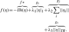
With the regularization and defining the shorthand notation |η|₁=∑_i,j |η_(i,j)| and ||η_i||₂=(∑_j η_(i,j)²)^(1/2), the overall objective f takes the form

We show that discretizing the data, X, to some precision β, and taking the limit as β→∞ has the equivalent minima (up to scaling and the zero set) by using X without discretization. Note that the gradient of the log-likelihood function takes the form

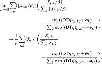which is the continuous extension of llh up to a constant . The regularization terms |η|₁, ||η||₂ and ||η||_TR are convex, but not strictly convex, so the optima of the continuous extension and the limit can differ up to elements of the zero set. Testing both small discretization and the continuous extension, we find no difference in results, but for completeness we use a threshold of 1e−5 to set a small neighborhood near zero to be part of the zero set.

Finally, we define the concept of an expression program as a set of basis vectors spanning η. The trace norm regularization implicitly penalizes the rank of matrix η, and for large λ₃, η will have small rank and can be represented as the linear combination of a few ‘basis’ programs. We choose the singular value decomposition of Tη as our program decomposition. The first k programs have a natural interpretation as the best rank-k approximation of the unnormalized log expression parameters.

Inference

The advantage of our method over topic model formulations is the convexity of our objective f, which guarantees fast convergence to the global maxima. Our overall inference strategy is to use gradient descent on the likelihood combined with proximal steps on each of the regularization terms. To speed convergence, we also use the accelerated proximal gradient method by.

The proximal gradient method allows us to efficiently optimize convex functions of the form f=f^*+g, where f^* is convex differentiable and g is convex and continuous. f is optimized with a gradient step on f^* followed by a proximal operator, which uses a quadratic approximation of f^* to optimize f^*+g. Given x_t, we generate the next iterate x_t+1 with the following update

In our case, our log likelihood is concave differentiable, and there are three convex continuous functions: g₁, g₂ and g₃, corresponding to each regularization term.

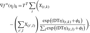
The gradient for f^* is given by the difference between predicted and observed counts

The proximal operators for g₁ and g₂ are the soft-threshold operators

For g₃, the proximal operator can be written in closed form in terms of its singular value decomposition (SVD) [14]. Let η=U DV^T and max(D−λ₃ϵ, 0) be the SVD and entrywise subtraction followed by thresholding, then the proximal operator takes the form

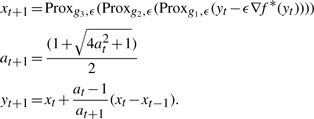
At each step of the optimizer, we take some x_t and step size ϵ and produce the next iterate with

The sequential proximal gradient converges for our objective due to separability. We also make use of the accelerated gradient method by, which finds a sequence of x_t which converges toward the optima, using an internal variable y_t and a magnification of the gradient, a_t to increase convergence rates near the mode.

In the context of a single proximal operator, this produces the optimal quadratic first-order convergence rate. In our case, the multiple proximal operators do not provide a guaranteed convergence rate, but in practice, we find the accelerated gradient makes convergence significantly faster. An implementation of this inference method as well as the results of our analysis are available from our website at http://psrg.csail.mit.edu/resources.html

For the remainder of the article we use a convergence tolerance of 10⁻⁵ and hot starts, which allows us to quickly find solutions over a list of candidate λ₁ values by using the optima of one problem to initialize a new problem with similar regularization penalties. This allows us to obtain the regularization path over λ₁ for the 105 array experiments below within 10 min on a computer with a Core 2 Duo e6300 CPU and 2 GB of memory.

Inference with this method is fast enough that we are able to fit the model across a 50×50×50 grid of all valid λ₁, λ₂ and λ₃, which we use to set the regularization parameters as described in the next section.

3 RESULTS

The algorithm was tested on directed differentiation experiments for murine pancreatic progenitors and motor neurons, as shown in Figure 4. Both lines were produced using known differentiation protocols. The pancreatic line has a large number of states, but relatively few replicates, while the motor neuron line has multiple replicates per state. The 88 microarray measurements of the pancreatic line were performed with Illumina bead arrays, while the 17 in the motor neuron line were performed with Affymetrix 430a2 microarrays. We rank-match the Illumina data to the Affymetrix data in order to reduce the data to the same scale.

Fig. 4.

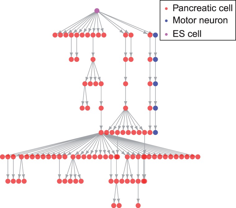
Murine differentiation tree representing the derivation of 88 pancreatic and 17 motor neuron expression measurements. Each edge is an experimental treatment and each vertex a experimental state

The quantile normalization technique is described in further detail by Irizarry et al (2003).

Cross-validation procedure

We use cross-validation to estimate the regularization parameters λ₁, λ₂ and λ₃ over the 50×50×50 grid of all nondegenerate values. For every experimental state with more than one observation, we include one observation in the training set and include the rest in the held-out set. We choose to leave out observations per-node rather than over all observations, since we must leave at least one observation at each node in order to make a prediction at the node. The performance of the model is measured in terms of held-out likelihood, which indicates goodness of fit, and squared error, measures predictive performance.

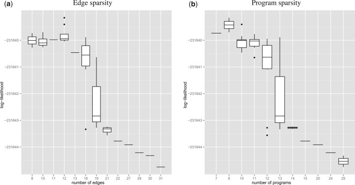
Cross-validation results in Figure 2 show the existence of a sharp drop in predictive power around a dozen edges and programs; this sharp transition suggests that there exists a necessary level of regularization for our algorithm to generalize well.

Fig. 2.

The goodness of fit as measured by held-out likelihood shows that the optimal model has few of edges and programs

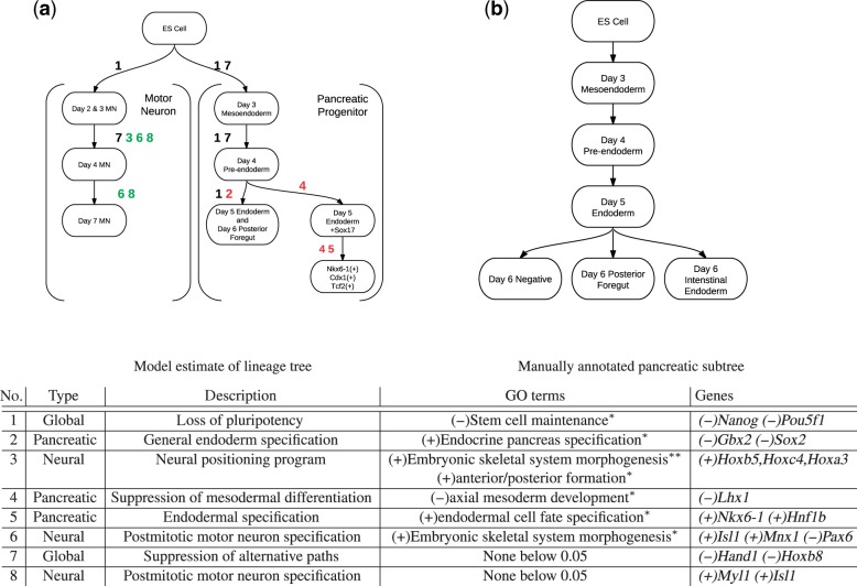
The optimal regularization parameters discovered by cross-validation significantly penalize both the number of edges and rank of the parameter η. At this optimal value, we find that the estimated cell state tree in Figure 8 is significantly sparser than the experimental tree. We also found that a strong L₁ penalty dominated the group L₂ penalties, resulting in λ₁ controlling both structural and parameter sparsity.

Fig. 8.

(Top) Estimated lineage tree for motor neuron and pancreatic progenitor; nodes are grouped by cell type and edges are labeled by program involved; color indicates program type (see table below) (Bottom) Major GO terms and Genes corresponding to developmental programs stars denote Benjamini–Hochberg corrected P-value of enrichment t-test; ^*P>0.05;^**P>0.01

Necessity of trace norm regularization

The trace-norm penalty is a critical part of modeling large branching factors. The L₁ and L₂ penalties shrink the changes between nodes to zero and bring the probabilities at each child-node toward their common parent. Therefore, the two edge penalties, λ₁ and λ₂, control whether leaves differ at all from their parent, rather than how they differ. In contrast, the trace norm penalty restricts directions in which the leaves can differ by forcing the leaves to lie within a small subspace near their parent.

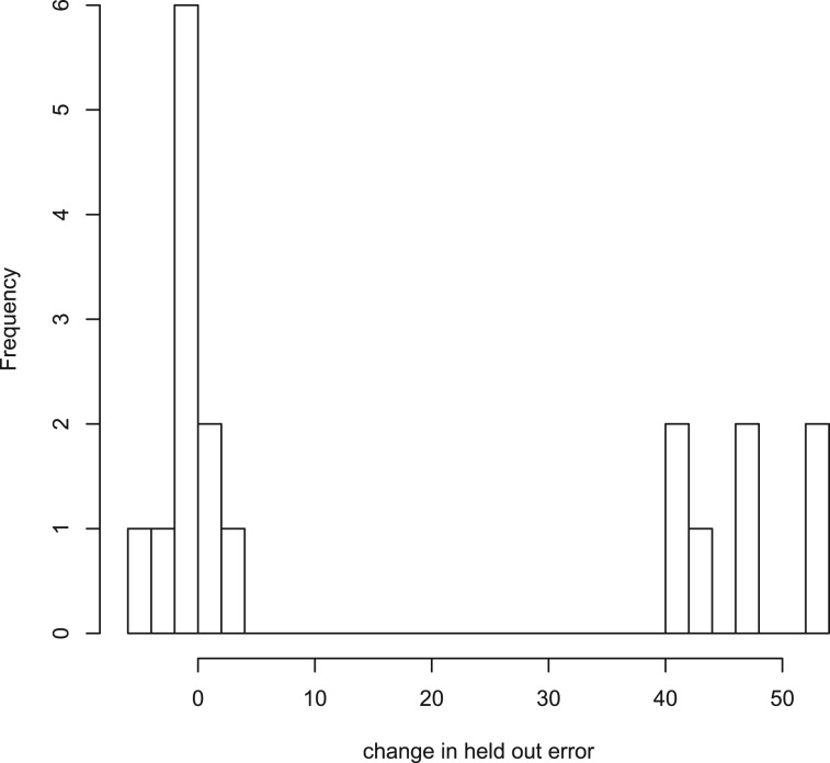
To test the necessity of trace norm regularization, we compared our model with and without trace-norm regularization. For both models, we fit the regularization parameters through cross-validation and compared the mean squared error on a common held-out set of 16 arrays selected by removing one array from each node with replicates. Results in Figure 5 indicate that without the trace norm penalty, 7 of the 16 held-out observations show significant increases in squared error. All seven of these observations are children of the highest degree node in Figure 8 suggesting that the trace norm penalty plays a key role preventing overfitting on highly branching data.

Fig. 5.

Measureing held-out error in models with and without trace norm penalty shows that removing trace norm penalty causes large increases in held-out error for 7 out of 16 held-out sets

Methods compared

Our algorithm was compared against three existing classes of approaches: SVD, non-negative matrix factorization (NMF) and latent Dirichlet allocation (LDA) on both held-out prediction error and quantitative program metrics. We were restricted to considering non-lineage-informed methods since we did not find any lineage informed methods in the literature.

For each competing method, we tested major variants of the algorithms and chose to compare only to the best variant. For SVD, we tried direct decomposition of the data, mean subtraction [resulting in Principal Component Analysis (PCA)] and mean subtraction on pancreatic and motor neuron branches; simple mean subtraction outperformed the others and is shown here. For NMF, we tested Kullback-Leibler (KL) divergence and square distance minimization objective proposed by as well as sparse NMF; we use KLdivergence minimization. For LDA, we used the collapsed Gibbs sampler as well as variational Bayes updates and found the Gibbs sampler with 20 000 samples to perform best.

Low cross-validation error on branching data

The held-out mean squared prediction error measures the generalization performance of each of the algorithms. We split the expression measurements into cross-validation and held-out sets selecting 16 replicate experiments one from each node with more than one measurement. The cross-validation set is split into training and test sets using the procedure described in the the cross-validation section. The models are fit on the training data and we calculate the squared error between the predicted values from the model and the test data.

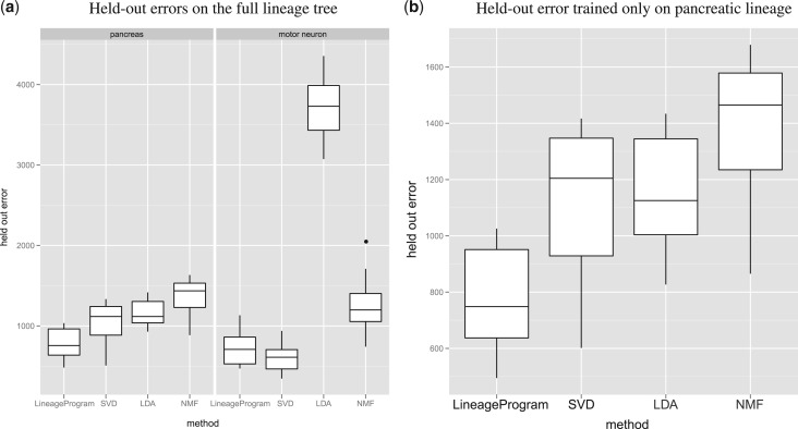
Training on the full set of motor neuron and pancreatic data (Figure 3a), we find that overall, LineageProgram has the lowest mean squared prediction error. On lineages with no branching, we would expect to see SVD perform best due to its direct minimization of squared error. We find that on the motor neuron lineage with no branching, our algorithm performs like SVD. In the worst case of non-branching data, our algorithm compares favorably to current factorization methods. Interestingly, LDA degenerates on the motor neuron held-out sets with behavior consistent on both training methods and across multiple replications. We find that LDA overfits on the later stage pancreatic states at the expense of the motor neuron states, which is consistent with behavior observed in prior work [8].

Fig. 3.

Cross-validated mean square errors on the full cell tree shows good predictive performance by LineageProgram

To rule out the possibility that the low performance of the competing algorithms was due to the inclusion of two differing array types in the pancreatic and motor lineages, we re-ran the test, fitting and evaluating only on the pancreatic lineage (Figure 3b).

The tests on the pancreatic lineage show nearly the same results for all methods, with all methods, particularly LDA, performing slightly better. However, the general ordering of the methods remains the same, and the performance results are due to the inability of current methods to handle the large branching factors in the pancreatic lineage rather than the combination of multiple lineages.

Comparison of program quality

Although methods such as SVD can reconstruct expression values well, these program decompositions are often difficult to interpret biologically. Therefore, we quantify the quality of the decomposition in terms of sparsity and biological relevance. First, we would hope for each program to have several dominant genes in order to produce candidate genes for further analysis. We measure this objective by the coefficient distribution of the programs. Second, we want each program to encode for biologically meaningful sets of genes. As with prior work [10], we measure Gene Ontology (GO) term enrichment as a proxy for biological relevance. Finally, we want each program to map to a unique developmental gene set. We measure this objective with the proportion of the program explained by the dominant developmental gene set.

Fewer genes are used to maodel the lineage

To measure sparsity, we normalize the programs from all methods to have unit norm and measure the L₂ norm of each gene over all programs. The L₂ norm is measure of average change in odds across programs. If there are a few genes dominating each program, we would expect to see only a few genes with high L₂ norm. Our goal is to recover interpretable programs, where each program contains a few key genes with large and unique activations. Our results in Figure 7 show that LDA and LineageProgram both produce a few large coefficients and a large number of coefficients within machine precision of zero. The dominance of few genes in each program allows us to label each program with a set of representative genes in Table 8.

Fig. 7.

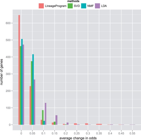
The distribution of average odds change over all programs per gene shows that LineageProgram produces sparse programs with many genes at zero and few dominant genes

Higher biological relevance of extracted programs

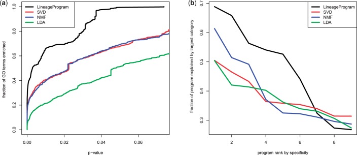
To measure the biological relevance of the discovered programs, we performed GO enrichment analysis using the weighted Kolmogorov statistic from gene set enrichment analysis. Plotting GO enrichment across all programs as a function of Benjamini Hochberg corrected P-values (Figure 6a), we find that LineageProgram achieves significantly higher GO enrichments when compared to the other methods. The higher GO enrichment across all P-values suggests that the programs recovered by LineageProgram more closely match subtrees of the GO annotation than those recovered by competing methods. If this were purely a result of chance, we would expect LineageProgram to outperform the others on a small subset of P-value cutoffs, rather than across all cutoffs. In combination with our sparsity results, this suggests that LineageProgram discovers small sets of biologically relevant genes in each program.

Fig. 6.

Gene set enrichment in Gene Ontology (GO) and manually curated developmental gene sets show programs recovered by LineageProgram are biologically relevant

To ensure that GO enrichment is in developmentally relevant categories, we also test the uniqueness of each program. In an ideal decomposition, each program would encode a different aspect of the developmental process. We use six developmental gene sets found in the literature, including four GO categories (‘stem cell maintenance’,‘endocrine pancreas differentiation’,‘embryonic skeletal development’, and ‘anterior posterior development’), as well as marker genes for motor neurons (Pax6, Mnx1, Isl1, Lhx1 and Lhx3) [13] and pancreas (Prox1, Pdx1, Hb9 and Nkx6-1) [15]. For each program, we measure the proportion of the program's L₂ norm that is accounted by genes in the most activated category. The results in Figure 6 show that LineageProgram as well as NMF have programs closesly matching known differentiation programs. These correspond to the loss of pluripotency; LDA and SVD were unable to discover programs that could be mapped solely to pluripotency. Importantly, LineageProgram maintains a relatively high correspondence to known gene sets across most of its programs, indicating its ability to encode small, highly specific gene modules corresponding to both the pancreatic and motor neuron lineages.

Analysis of full lineage data

Finally, we train LineageProgram on the full dataset to estimate lineage programs and use cross-validation on replicates to estimate regularization parameters. The resulting tree is sparse, with only two branching points (Figure 8). The first branching point corresponds to the split between motor neuron and pancreatic lineages. The other branching point differentiates a successful Day 6 pre-endoderm differentiation from a late-stage Sox17 overexpression experiment.

We compared the lineage tree from the model with a manual annotation produced separately from this project. Taking only the vertices corresponding to known cellular states, we match the manual curation almost exactly, successfully reducing all the branches before the Day 4 preendoderm and only mis-merging the Day 5 endoderm with the Day 6 posterior foregut. The regularization and cross-validation have successfully pruned nearly all spurious branches of the linage tree.

The Sox17 branch in Figure 8 represents a late-stage experiment aimed at recovering competency in Day 8 endoderm using Sox17 overexpression. Although the experiment shows significant expression level differences from the Day 4 pre-endoderm, we have not positively identified this state as a biologically significant cell state.

Identification of enriched GO terms and genes also show close correspondence with known biological facts. We correctly identify all major stages of the motor neuron differentiation process, from loss of pluripotency and development of positional identity to spinal motor neuron specification. On the pancreatic branch, we identify loss of pluripotency, suppression of mesodermal identity and finally specification of endodermal and pancreatic identity. We include full summary output of the enriched genes and GOs for each program in the appendix.

CONCLUSION

We have presented LineageProgram, a log-linear sparse regularized model and inference algorithm for lineage-associated expression data that provide strong interpretability with no loss in predictive power. Existing flat modeling methods were unable to cope with the large number of leaves that occur at the ends of the differentiation experiment, and significant statistical power is lost re-estimating the background cellular expression levels. Our biological metrics also suggest that flat factorization methods do not extract biologically meaningful expression programs, and modeling the differences between each differentiation state is necessary to estimating fine behaviors occuring during differentiation.

Our analysis of the combined pancreas and motor neuron data provides a computational analysis of the pancreatic and motor neuron differentiation pathways that recapitulate known biological markers and states. The ability of the sparse regularization to remove spurious branches in the lineage tree suggests the use of this model to estimate novel cellular states in later-stage differentiation experiments, where explicit cellular states are less characterized.

Although we have restricted our model to expression-based data, we hope to extend this framework of L₁-regularized branching models to sequencing data with similar structure. The penalty model presented here would allow a wide variety of log-convex generative models to incorporate lineage-associated structure.

Funding: National Institutes of Health [P01-NS055923 and 1-UL1-RR024920 to D.K.G.].

Conflict of Interest: none declared.

REFERENCES

- Akashi K., et al. Transcriptional accessibility for genes of multiple tissues and hematopoietic lineages is hierarchically controlled during early hematopoiesis. Blood. 2003;101:383–389. doi: 10.1182/blood-2002-06-1780. [DOI] [PubMed] [Google Scholar]
- Alter O., et al. Singular value decomposition for genome-wide expression data processing and modeling. Proc. Na. Acad. Sci. USA. 2000;97:10101–10106. doi: 10.1073/pnas.97.18.10101. [DOI] [PMC free article] [PubMed] [Google Scholar]
- Bar-Joseph Z., et al. Analyzing time series gene expression data. Bioinformatics. 2004;20:2493–2503. doi: 10.1093/bioinformatics/bth283. [DOI] [PubMed] [Google Scholar]
- Carmona-Saez P., et al. Biclustering of gene expression data by non-smooth non-negative matrix factorization. BMC Bioinformatics. 2000;7:78. doi: 10.1186/1471-2105-7-78. [DOI] [PMC free article] [PubMed] [Google Scholar]
- Cheng Y, Church G.M. Proceedings / … International Conference on Intelligent Systems for Molecular Biology. Vol. 8. ISMB; 2000. Biclustering of expression data; pp. 93–103. International Conference on Intelligent Systems for Molecular Biology. [PubMed] [Google Scholar]
- Costa I., et al. Gene expression trees in lymphoid development. BMC Immunology. 2007;8:25. doi: 10.1186/1471-2172-8-25. [DOI] [PMC free article] [PubMed] [Google Scholar]
- Ivan Costa G., et al. Inferring differentiation pathways from gene expression. Bioinformatics. 2008;24:i156–i164. doi: 10.1093/bioinformatics/btn153. [DOI] [PMC free article] [PubMed] [Google Scholar]
- Eisenstein J., et al. Sparse additive generative models of text. 2011 [Google Scholar]
- Ferrari F., et al. Genomic expression during human myelopoiesis. BMC Genomics. 2007;8:264–264. doi: 10.1186/1471-2164-8-264. [DOI] [PMC free article] [PubMed] [Google Scholar]
- Georg K., et al. Automated discovery of functional generality of human gene expression programs. PLoS Computational Biology. 2007;3:e148. doi: 10.1371/journal.pcbi.0030148. [DOI] [PMC free article] [PubMed] [Google Scholar]
- Hoyer P.O. Non-negative matrix factorization with sparseness constraints. J. Machine Learn. Res. 2004;5:1457–1469. [Google Scholar]
- Irizarry R.A., et al. Exploration, normalization, and summaries of high density oligonucleotide array probe level data. Biostatistics. 2003;4:249. doi: 10.1093/biostatistics/4.2.249. [DOI] [PubMed] [Google Scholar]
- Jessell T.M. Neuronal specification in the spinal cord: inductive signals and transcriptional codes. Nature Reviews Genetics. 2000;1:20–29. doi: 10.1038/35049541. [DOI] [PubMed] [Google Scholar]
- Ji S., Ye J. Proceedings of the 26th Annual International Conference on Machine Learning. ACM; 2009. An accelerated gradient method for trace norm minimization; pp. 457–464. [Google Scholar]
- Jørgensen M.C., et al. An illustrated review of early pancreas development in the mouse. Endocrine reviews. 2007;28:685. doi: 10.1210/er.2007-0016. [DOI] [PubMed] [Google Scholar]
- Joung J.-G., et al. Identification of regulatory modules by co-clustering latent variable models: stem cell differentiation. Bioinformatics. 2006;22:2005–2011. doi: 10.1093/bioinformatics/btl343. [DOI] [PubMed] [Google Scholar]
- Lee D.D., Seung H.S. Algorithms for non-negative matrix factorization. Advances in neural information processing systems. 2001;13:788–791. [Google Scholar]
- Martins A.F.T., et al. Online learning of structured predictors with multiple kernels. Proceedings of the 14th International Conference on Artificial Intelligence and Statistics. 2011 [Google Scholar]
- Mazzoni E.O., et al. Embryonic stem cell-based mapping of developmental transcriptional programs. Nature methods. 2011 doi: 10.1038/nmeth.1775. [DOI] [PMC free article] [PubMed] [Google Scholar]
- Medvedovic M., et al. Bayesian mixture model based clustering of replicated microarray data. Bioinformatics (Oxford, England) 2004;20:1222–1232. doi: 10.1093/bioinformatics/bth068. [DOI] [PubMed] [Google Scholar]
- Nesterov Y., Nesterov I.U.E. Introductory Lectures on Convex Optimization: A Basic Course. Applied optimization. Kluwer Academic Publishers, MA, USA.; 2004. [Google Scholar]
- Niakan K.K., et al. Sox17 promotes differentiation in mouse embryonic stem cells by directly regulating extraembryonic gene expression and indirectly antagonizing self-renewal. Genes & Development. 2010;24:312. doi: 10.1101/gad.1833510. [DOI] [PMC free article] [PubMed] [Google Scholar]
- Subramanian A., et al. Gene set enrichment analysis: a knowledge-based approach for interpreting genome-wide expression profiles. Proc. Nat. Acad. Sci. USA. 2005;102:15545. doi: 10.1073/pnas.0506580102. [DOI] [PMC free article] [PubMed] [Google Scholar]
- Wirth H., et al. Expression cartography of human tissues using self organizing maps. BMC Bioinformatics. 2011;12:306. doi: 10.1186/1471-2105-12-306. [DOI] [PMC free article] [PubMed] [Google Scholar]
- Zagar L., et al. Stage prediction of embryonic stem cell differentiation from genome-wide expression data. Bioinformatics. 2011;27:2546–2553. doi: 10.1093/bioinformatics/btr422. [DOI] [PubMed] [Google Scholar]
- Zhang B., et al. Estimating developmental states of tumors and normal tissues using a linear time-ordered model. BMC Bioinformatics. 2011;12:53. doi: 10.1186/1471-2105-12-53. [DOI] [PMC free article] [PubMed] [Google Scholar]