NOrMAL: accurate nucleosome positioning using a modified Gaussian mixture model

Abstract

Motivation: Nucleosomes are the basic elements of chromatin structure. They control the packaging of DNA and play a critical role in gene regulation by allowing physical access to transcription factors. The advent of second-generation sequencing has enabled landmark genome-wide studies of nucleosome positions for several model organisms. Current methods to determine nucleosome positioning first compute an occupancy coverage profile by mapping nucleosome-enriched sequenced reads to a reference genome; then, nucleosomes are placed according to the peaks of the coverage profile. These methods are quite accurate on placing isolated nucleosomes, but they do not properly handle more complex configurations. Also, they can only provide the positions of nucleosomes and their occupancy level, whereas it is very beneficial to supply molecular biologists additional information about nucleosomes like the probability of placement, the size of DNA fragments enriched for nucleosomes and/or whether nucleosomes are well positioned or ‘fuzzy’ in the sequenced cell sample.

Results: We address these issues by providing a novel method based on a parametric probabilistic model. An expectation maximization algorithm is used to infer the parameters of the mixture of distributions. We compare the performance of our method on two real datasets against Template Filtering, which is considered the current state-of-the-art. On synthetic data, we show that our method can resolve more accurately complex configurations of nucleosomes, and it is more robust to user-defined parameters. On real data, we show that our method detects a significantly higher number of nucleosomes.

Availability: Visit http://www.cs.ucr.edu/~polishka

Contact: stelo@cs.ucr.edu or polishka@cs.ucr.edu

1 INTRODUCTION

The study of the processes governing gene regulation is a central problem in molecular biology. One of the key factors influencing gene expression is the complex interaction between chromatin structure and transcription factors. The fundamental unit of chromatin is the nucleosome, composed of 146 ± 1 bp of DNA wrapped 1.65 turns around a protein complex of eight histones. To elucidate the role of the interactions between chromatin and transcription factors, it is crucial to determine the location of the nucleosomes along the genome. In general, the more condensed the chromatin, the harder it is for transcription factors and other DNA binding proteins to access DNA and carry out their tasks. The more accessible is the DNA, the more likely surrounding genes are actively transcribed. The presence (or the absence) of nucleosomes directly or indirectly affects a variety of other cellular and metabolic processes like recombination, replication, centromere formation and DNA repair.

A handful of experimental techniques have been developed for genome-wide mapping of nucleosomes. For instance, one can enrich for genomic regions that are either bound to histones (typically via chromatin immuno-precipitation or ChIP) or for genomic regions that are free of nucleosomes (linkers). For instance, MAINEs (MNase-assisted Isolation Nucleosomal Elements) (Zaret, 2005) isolates the portions of the DNA that are attached to nucleosomes, because MNase preferentially digests linker regions. Then, microarrays (ChIP-chip) or sequencing (ChIP-seq/MNase-seq) are applied to the enriched DNA.

In this article, we concentrate on the analysis of sequencing data, given the prevalence of MNase/ChiP-seq experiments in the recent literature. The computational analysis of the sequencing data usually consists of two main steps: (i) a nucleosome occupancy coverage is computed from the process of mapping nucleosome-enriched sequenced reads to a reference genome, followed by some normalization steps and (ii) nucleosomes are placed according to the peaks of the coverage profile.

Approaches based on peak calling are computationally fast and quite accurate in resolving isolated (stable or arrayed) nucleosomes; however; they are not entirely reliable when more complex nucleosome configurations are present. Observe that while it is physically impossible for two nucleosomes to be ‘overlapping’ on the same location on a DNA strand, it is quite common that the population of cells from which the enriched DNA was obtained had nucleosomes slightly ‘off-sync’ at a given genomic coordinate (transient interaction). As a consequence, the resulting coverage profile will exhibit a ‘blurring’ of the peaks.

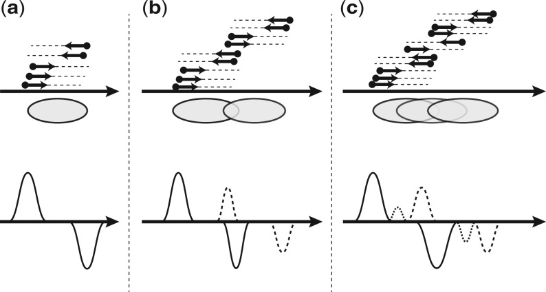
Molecular biologists distinguish the case of ‘overlapping’ nucleosome from ‘fuzzy’ nucleosomes or ‘fuzzy’ regions (see Fig. 1). For overlapping nucleosomes, the overlap is relatively small; in the ‘fuzzy’ case, several nucleosomes are mutually overlapping for a significant fraction of their size (see Zhang and Pugh, 2011 for a review). By introducing a threshold parameter on the allowed overlap, one can define precisely the line between ‘fuzzy’ and ‘overlapping’.

Fig. 1.

Nucleosomes are represented by ovals, mapped reads by arrows (which correspond to 5′→3′ prefixes of nucleosome-bound DNA). Coverage profiles are represented as time series for forward (top) and reverse (bottom) strands: the line style (solid, dotted and dashed) indicates peaks originating from distinct nucleosomes. (a) represents a stable nucleosome; (b) illustrates overlapping nucleosomes; and (c) represents ‘fuzzy’ nucleosomes

Another shortcoming of peak-calling approaches is that they can only report nucleosome positions and/or occupancy level. Molecular biologists, however, need additional information about nucleosomes. For instance, they are interested in the level of ‘fuzziness’ in certain genomic locations with respect to coding regions (i.e. well positioned for all the cells in the sample, or ‘blurred’), or how strong is the binding between nucleosomes and DNA. To address these shortcomings, we propose a method that determines the accurate position of the nucleosomes independently from the amount of overlaps in the nucleosomes. This method can also extract other important statistics about nucleosomes, e.g. the probability that a nucleosome is actually present, a measure of nucleosome ‘fuzziness’, and the size of DNA fragments enriched for nucleosomes.

Here, we propose a parametric probabilistic model for nucleosome positioning, which we called NOrMAL, for NucleOsome Mapping ALgorithm. NOrMAL uses Expectation Maximization (EM) to infer its parameters. To demonstrate the performance of our method, we report experimental results on MAINE-seq data for Plasmodium falciparum (Ponts et al., 2010) and Saccharomyces cerevisiae (Weiner et al., 2010). We compare the performance of our method against the Template Filtering (TF) algorithm (Weiner et al., 2010), which is considered the current state-of-the-art in terms of accuracy and ability to estimate sizes of the DNA fragments bound to nucleosomes. We also discuss a fundamental limitation of greedy peak-calling approaches in the case of overlapping nucleosomes and how our method addresses this issue.

1.1 Previous work

Several landmark studies have been published in the last few years on the chromatin structure of model organisms based on the analysis of genome-wide nucleosome maps (Albert et al., 2007; Field et al., 2008; Mavrich et al., 2008a, b; Ponts et al., 2010; Shivaswamy et al., 2008; Valouev et al., 2008; Zhang and Pugh, 2011). Existing methods in the literature are based on the analysis of the peaks in the nucleosome occupancy coverages estimated by mapping nucleosome-enriched reads to the reference genome. The coverage occupancy profile is an integer-valued function defined for all genomic locations: given a position i in a chromosome the function is equal to the number of sequenced reads that are mapped to location i. From a probabilistic point of view, the coverage profile represents a non-parametric distribution of the nucleosome positions. At the time of writing, the length of the reads obtained by second-generation sequencing (e.g. Illumina Genome Analyzer) are limited to about 100 bases and the sequencing occurs in the 5′→3′ direction. In the case of ChIP-seq/MAINE-seq, sequenced reads that can be uniquely mapped to the positive strand originate from the left boundary of nucleosome DNA fragments, while reads uniquely mapped to the negative strand originate from the right boundary (Fig. 1). Recall that nucleosomes are composed of about 146 bp of DNA, so if reads are single end and shorter than 146 bp, we expect to observe a peak in the forward and a peak in the reverse coverage profiles at a distance consistent with the nucleosome size.

The problem of associating a peak in the forward strand with the correct peak in the negative strand can be difficult in the case of a large number of complex nucleosome configurations. Some authors artificially extend the reads in the 5′→3′ direction or they shift the positions of the mapped read position of the forward and reverse toward the middle of potential nucleosomes. Then, they combine (e.g. sum) the forward and reverse modified coverages to build a score function. In both cases, they need to determine the amount of the extension or the size of the shift. In the former case, the extension should account for the expected length of the DNA fragments enriched for nucleosomes; in the latter, the shift should be about half of the DNA fragment size. The problem of this approach is that no extension or shift that will work equally well for all nucleosomes in the genome. While one should expect DNA fragments enriched for nucleosomes to be ~146 bp, the reality is that the digestion process can either leave nucleosome-free DNA in the sample, or ‘over-digest’ the ends of nucleosome-bound DNA. What complicates the matter further is that the rate of digestion is sequence dependent (Allan et al., 2012; Weiner et al., 2010), so nucleosomes in different genomic locations will end up with different DNA fragment size. For this reason, it is advantageous to ‘learn’ this information from the input data. TF (Weiner et al., 2010) is the only method we know that can handle variable fragment sizes in a specified range, whereas other methods require users to decide this value in advance.

As said, a variety of peak-calling algorithms have been also developed (Albert et al., 2007; Field et al., 2008, 2009; Kaplan et al., 2009; Mavrich et al., 2008a, b; Sasaki et al., 2009; Valouev et al., 2008). Most of these methods have been proposed for the analysis of ChIP-chip or ChIP-seq data to determine the position and strength of the transcription factors binding to DNA. The problem of detecting transcription factor binding sites is similar to nucleosome positioning: in both cases we need to infer position of proteins binding to DNA from the coverage profiles. However, the size of the nucleosomes is significantly bigger than transcription factor binding sites, as a consequence the resulting configurations of nucleosomes can be more complex.

To summarize our experience with existing methods on the genome-wide nucleosome study of human malaria parasite (Ponts et al., 2010, 2011), peak calling approaches suffer from a variety of problems. First, the coverage profile function has to be cleaned of high-frequency noise, typically via a kernel density estimation method (Parzen, 1962). The type of kernel and the amount of smoothing can drastically affect the results: too much can merge adjacent peaks, too little can leave too many noisy artifacts that can be interpreted as individual peaks. Second, peak finding algorithms have parameters (like the extension and the shift discussed above) that are difficult to optimize: a set of parameter can work for a region of a chromosome but not for another. Third, peak calling do not properly resolve overlapping nucleosomes. For instance, TF (Weiner et al., 2010) uses a greedy strategy: nucleosomes are placed according to the ‘best’ matching peaks in the score function. Once these strong-positioned nucleosome are assigned, TF ignores any nucleosome that overlaps with previous ones. It is relatively easy to show that for overlapping nucleosomes the greedy strategy does not always return the best overall placement (see Section 3 for details).

2 METHODS

Next, we propose a parametric probabilistic model to find the most likely set of nucleosome that best ‘explain’ the mapped reads. We cast this problem in a modified Gaussian mixture model framework. The problem of positioning nucleosomes is then reduced to the problem of learning the parameters of the model and finding the distribution of mixture components, which is achieved via EM.

2.1 A probabilistic model for nucleosomes

We employ a probabilistic model for nucleosome positioning that is described by a set of hidden and observed variables. We use N to denote the number of DNA fragments obtained after MNase digestion. For any DNA fragment i∈[1, N], let x_i be the starting position of the 5′-end of fragment i (obtained by mapping a corresponding sequenced read), and let variable d_i∈{+1, −1} be the strand on which fragment i was mapped (+1 for the positive strand, and −1 for the negative strand). Also, let z_i be the length of fragment i. If we use variable m_i to denote the position of the center of the fragment i, then we have m_i=x_i+(d_iz_i)/2.

We denote with X_i, D_i, Z_i and M_i the random variables associated with variables x_i, d_i, z_i and m_i, respectively. Since the sequencing process is 5′→3′, the value of X_i is observable by means of mapping a read originating from fragment i. Similarly, the strand variable D_i is also observable. Variables Z_i and M_i can be observed directly only if sequencing produces paired-end reads, otherwise these variables are hidden. In order to consider the most general case, we only deal with the latter case (single-end reads).

We assume for the time being that the number K of nucleosomes is given. We will discuss how to choose K in Section 2.3. For each DNA fragment i, we use a hidden variable C_i∈[1, K] representing the nucleosome to which it belongs. Each nucleosome j∈[1, K] is described by a set of six variables (μ_j, σ_j, Δ_j, δ_j⁺¹, δ_j⁻¹, π_j), where μ_j denotes the center position of the nucleosome j, σ_j is the fuzziness associated with the position of nucleosome j, Δ_j describes the length of DNA fragments associated with nucleosome j, δ_j⁺¹ and δ_j⁻¹ represents the variation on fragment sizes for positive and negative strands, respectively, and π_j is the probability of nucleosome j. The degree of fuzziness captures the variation of the position of a particular nucleosome in the population of sampled cells. Well-positioned nucleosomes have very low degree of fuzziness. We introduce two variables δ_j⁺¹ and δ_j⁻¹ to model the variation of the fragment size because MNase does not only digest nucleosome-free DNA. Given enough time, it can also digest into the ends of the fragments bounds to nucleosomes, the rate of digestion being sequence dependent [see, e.g. (Allan et al., 2012; Weiner et al., 2010)]. Since the sequence composition of the 5′ end of a DNA fragment can be quite different from the 3′ end, we need to have two different variables. The value of C_i is drawn from (1, 2,…, K) with corresponding probabilities (π₁, π₂,…, π_K). Parameter π_j models the contribution of j-th nucleosome to the occupancy level, i.e. what portion of the mapped reads belong to nucleosome j.

Our nucleosome model assumes that our random variables are distributed according to a normal distribution. For convenience of notation, we set Θ_j=(μ_j, σ_j, Δ_j, δ_j⁺¹, δ_j⁻¹, π_j) for all j∈[1, K], and Θ=(Θ₁,…, Θ_K). First, we assume that variable M_i associated with the center of the fragment i for a particular nucleosome j is distributed as follows

(1)

where μ_j represents the center of the nucleosome j and σ_j is its fuzziness. Second, we assume that the length Z_i of fragment i for a particular nucleosome j is distributed as follows

(2)

where Δ_j represents the expected size of the fragments for nucleosome j, and δ_j⁺¹ and δ_j⁻¹ represents the variation of fragment sizes for positive and negative strands, respectively.

Combining Equations (1) and (2) and relation x_i=m_i−(d_iz_i)/2, and then applying the rule of linear combination of independent Gaussians we obtain

(3)

Equation (3) allows one to compute the probability of a given data point x_i given the parameters of a nucleosome. Next, we describe the model for multiple nucleosomes.

2.2 Mixture model

Next, we introduce a generative mixture model to describe the likelihood of input data points X=(x₁,…, x_N). Figure 2 shows a graphical representation of the mixture model. In Equation (3), the only hidden random variable is C because we already excluded variables z_i from the computation. By grouping variables X_i, D_i, we can use an approach similar to a naive Bayes classifier. Variable C represents the nucleosome to which the points belong. Thus, we can describe the likelihood of point (x_i, d_i) given the parameters of our model as a mixture of distributions. Using the Bayesian rule we obtain

(4)

where is the Gaussian density function.

Fig. 2.

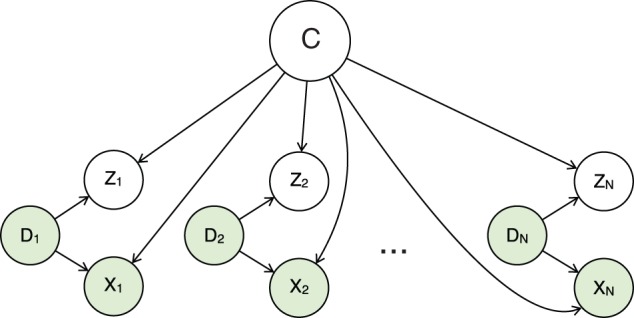
The proposed graphical mixture model: shaded nodes correspond to observed variables, white nodes correspond to hidden variables

Using Equation (4), we can obtain the log likelihood of observed data points X given parameters Θ as

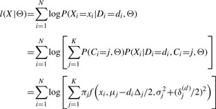(5)

Given Equation (5) and the input data points X=(x₁,…, x_N), we can find an estimate the parameters of the model Θ via maximum likelihood

(6)

Recall that Θ=(Θ₁,…, Θ_K) is a vector whose components are the nucleosome parameters Θ_j=(μ_j, Δ_j, σ_j, δ_j⁽⁺¹⁾, δ_j⁽⁻¹⁾, π_j) for all j∈[1, K]. The presence of parameters π_j that correspond to hidden variables C_i prevents us from solving Equation (6) directly. We estimate via EM. In our case, the E step requires computing the posterior probabilities P(C_i=j|X_i=x_i; Θ) of data points x_i, i∈[1, N] with respect to the distribution of C_i given the current estimate of parameters Θ^(t)

(7)

During the E step, we supplement the missing data in Equation (6) with the expected values under the current parameter estimates Θ^(t). In the M step, we find new parameter estimation Θ^(t+1) by maximizing Equation (7)

(8)

It is relatively straightforward to bound the variation parameters (σ, δ⁺¹, δ⁻¹) during the iterative EM process to converge to a solution with ‘reasonable’ parameters. We can also easily introduce prior distribution for some of the parameters. For instance, we can specify an expected distribution for DNA fragment sizes Δ_j, which can be estimated via gel electrophoresis prior to sequencing.

2.3 Choosing the number of nucleosomes

The method described above assumes that the number of clusters K is known. The problem of selecting the best value for K is as challenging as selecting the optimal number of clusters in k-means clustering. One can estimate the number of clusters by looking at the support area of the occupancy coverage, but this will be quite inaccurate because ‘fuzzy’ nucleosomes correspond to wider peaks, and the support area is bigger for them.

Here, we propose a simple but effective heuristic to find K. We start by (1) placing the maximum possible number of non-overlapping nucleosomes uniformly distributed on the chromosome, that is K= (size of the chromosome)/(expected size of a nucleosome), where the expected size of nucleosomes is underestimated. Then, (2) we run our EM algorithm until convergence (‘soft learning’). We will then (3) check the distance between the clusters, and merge those that have too much overlap (above a user-specified threshold). In case of multiple overlaps for a nucleosome, we merge it with the closest one. We repeat (2) and (3) until no additional clusters are merged. After a few cycles, we will obtain a set of non-overlapping clusters that best explain the given data points. Overlapping nucleosomes are merged into new ones and then the position of new nucleosomes are learned from the data.

This procedure will give us a good estimate on the number of clusters as well as a rough estimate of the nucleosome positions. To further improve accuracy for other model parameters, we perform one iteration of ‘hard learning’ by assigning each data point x_i its maximum probable cluster. Nucleosome clusters will partition the set of input points, which in turns will allow us to compute their parameters more accurately. The pseudo-code of the algorithm is shown on Figure 3. The running time of NOrMAL is dominated by the running time of Learning step (Algorithm 1, line 6). Observe that the probability that a data point belongs to far-away nucleosomes is close to zero, so one can avoid unnecessary computations by computing updates only for clusters in close vicinity of each point.

Fig. 3.

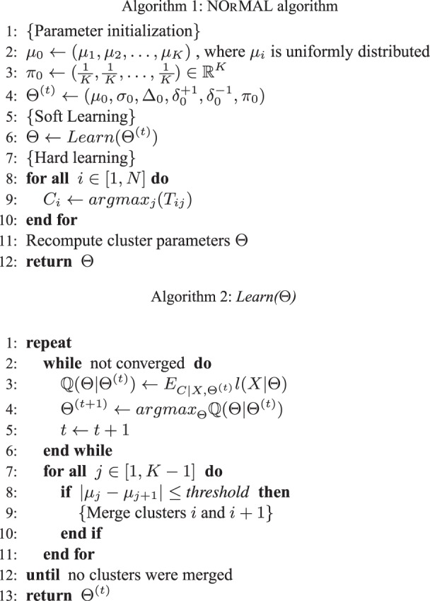
A sketch of the proposed NOrMAL algorithm

The running time is dominated by the heuristic used to find the number of nucleosomes K. In order for the algorithm to scale to eukaryotic genomes, additional optimization steps will have to be implemented. For instance, during the early stage of soft learning (i.e. active cluster merging), the algorithm could be applied to small ‘chunks’ of chromosomes. Then, when the number of merges reduces substantially, the nucleosome maps for each chunk could be combined and algorithm would continue to the hard-learning step.

2.4 Practical considerations

Our method requires users to specify three parameters, namely the threshold for allowed overlap between adjacent nucleosomes, the prior Δ on nucleosome sizes and its weight λ.

The threshold for allowed overlap can significantly affect the output: the more overlap is allowed, the more nucleosomes can be placed. In the current implementation, this parameter has to be specified by the user. The prior Δ on the nucleosome size and its weight λ control the propagation of ‘knowledge’ from data points on forward strand to data points on the reverse strand, and vice versa. Based on our experience, if the prior size Δ is within 30 bp of the ‘true’ fragment size, then the algorithm is consistent in its output.

Our implementation has some additional internal parameters that we are not expecting users to change. While inferring the parameters of our mixture models, some clusters will tend to cover most of the data points using large variances: a common trick to avoid this from happening is to introduce hard limits on such parameters. Our implementation has range limits for the nucleosome sizes and variance to force the method to converge to ‘reasonable’ nucleosome sizes/variances in the early stage of the iterative process. These parameters have been chosen loose enough so by the end of the iterative process, the limits for nucleosome size and variance are rarely hit, and the output is not significantly affected. The hard-learning step completely ignores those upper limits.

Additional details on parameter selection will be found in the on-line User Manual.

3 EXPERIMENTAL RESULTS

We carried out extensive benchmarking between our proposed method NOrMAL and TF (Weiner et al., 2010). We selected TF because it is considered the current state-of-the-art. It is the only method that, in addition to inferring nucleosome positions, can extract nucleosome fragment sizes and binding scores. TF differs from the traditional peak-calling algorithms because it does not look for peaks in the coverage profiles, but it places nucleosomes at the peaks of a correlation score matrix. Due to its greedy strategy, TF has significant limitations when dealing with fuzzy/overlapping nucleosomes, as explained next.

The setup for the comparison is as follows. The input parameters for NOrMAL are the prior size of the nucleosome fragments and the allowed amount of overlap between nucleosomes. For TF, we used default parameters unless specified otherwise. The default allowed range of nucleosome size for TF is [100,200], which centered around the expected nucleosomes size of ~146 bp.

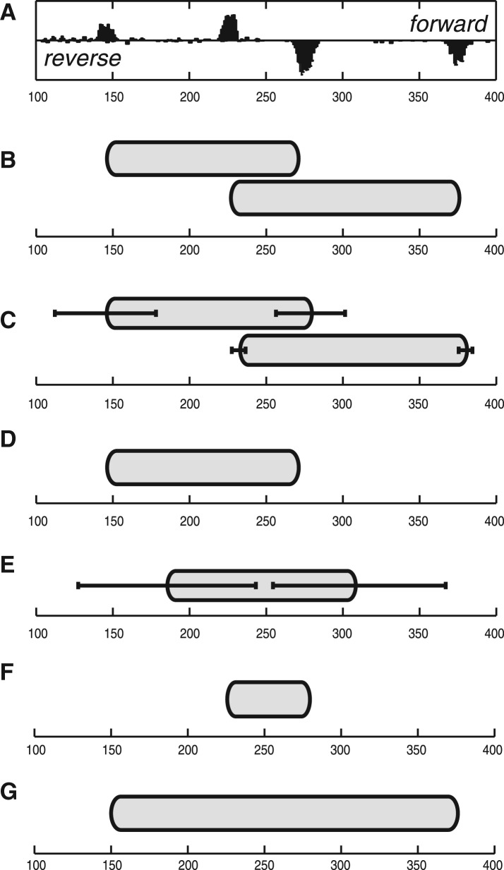
Synthetic data: first, we want to illustrate the challenge for existing nucleosome positioning methods to deal with the placement of overlapping nucleosomes. The problem derives from the difficulty in distinguishing two overlapping nucleosomes from the ‘fuzzy’ case. To define precisely this problem, we need to introduce a threshold parameter: if the percentage of overlap between two nucleosomes exceeds the threshold, then they should be considered ‘fuzzy’, otherwise they should be treated as separate overlapping nucleosomes. It is relatively easy to show that the greedy strategy does not always give the optimal nucleosome placement in case of overlapping nucleosomes. To do so, we have created a small synthetic dataset that contains reads corresponding to two overlapping nucleosomes. Although we could have used our own parametric model to generate the synthetic data, to avoid the possibility of giving an advantage to our method, we generated the input data according to the template function described in (Weiner et al., 2010). The parameters for nucleosome positions (μ₁ and μ₂) and nucleosome sizes (Δ₁ and Δ₂) that we used to generate the reads are reported in Table 1. Figure 4A illustrates the coverage profile for mapped reads. Observe that there are two peaks on forward and reverse strands, which indicates the presence of two nucleosomes. The percentage of overlap is roughly 35%. In the first case, we allowed such amount of overlap in both TF and NOrMAL (Fig. 4B for TF and Fig. 4C for NOrMAL). Both methods correctly reported two overlapping nucleosomes. Observe the error bars attached to the boundaries of nucleosomes reported by NOrMAL, which indicate the positional variance (or ‘fuzziness’) of the corresponding boundary (each bar has length ). TF does not provide such information.

Table 1.

The parameters used to generate the reads in Figure 4, and the corresponding output results from TF and NOrMAL

Parameter	True value	TF	NOrMAL
μ1	210	208	206
Δ1	130	125	134
μ2	300	301	300
Δ2	150	149	148

Fig. 4.

An example of two overlapping nucleosomes. (A) Coverage profile from synthetic data (forward strand on top, reverse strand on bottom), where nucleosomes overlap on ~35 of their length; nucleosomes detected using TF allowing maximum 35% overlap (B), NOrMAL allowing maximum 35% overlap (C), TF allowing only 30 overlap, [100,200] (D) and NOrMAL allowing only 30% overlap (E); nucleosome reported by TF with nucleosome size range [40,200] (F) and [100,300] (G)

In the second case, when the parameters are set so nucleosomes are not allowed to overlap >30%, only one nucleosome should be reported. Figure 4D and E illustrates the output of TF and NOrMAL, respectively. Observe that now there is a fundamental difference: TFs greedy strategy reports the presence of the first nucleosome, but then it completely ignores the data corresponding to the second nucleosome. This is an entirely arbitrarily choice and the user will not be even aware of this. In contrast, NOrMAL reports one nucleosome positioned near the centroid of the data points and correctly indicates that the variance of the nucleosome boundaries in this case is very high, indicating that this nucleosome should be considered ‘fuzzy’.

In addition, TFs positioning results are very sensitive to its main input parameter, namely the allowed range for nucleosome fragment sizes. With the default size range [100,200], TF reports one nucleosome (Fig. 4D). When we extend the range to [40,200], TF detects one small nucleosome by incorrectly matching the two strongest (but closest) peaks (Fig. 4F). If we change the range to [100,300], TF reports one large nucleosome, this time matching the outmost peaks (Fig. 4G). Even if we allow a larger overlap, TF will still produce the nucleosome in Figure 4G (data not shown). Since the allowed range for nucleosome size in TF is a hard boundary, the results are very dependent from the choice of this parameter. NOrMAL is more robust in that regard because the prior distribution for the fragment sizes in NOrMAL is ‘soft’ and it can adapt to the data.

Real data: the challenge for nucleosome position inference is that the true positions of the nucleosomes are unknown. The lack of a ‘ground-truth’ makes it very hard to benchmark the existing computational methods. To compare between methods, we can only use conservative indicators. We argue that a valuable indicator is the number of reported nucleosomes. Nonetheless, it is difficult to argue about performance in objective terms. That is why the first dataset we considered is from S. cerevisiae (Weiner et al., 2010). This was the original dataset for which TF was designed. The results of TF on this dataset are assumed to be accurate.

To compare NOrMAL and TF, we used the following setup. The main range parameter for TF was set to [80,200], which is slightly wider than the default parameters. We did not want to penalize TF, since NOrMAL does not have any hard limits for the nucleosome sizes. For NOrMAL, the main parameter is the prior expected value for the nucleosome sizes: we used 140 bp to hit the middle of the specified range of TF. The threshold value of allowed overlap for both methods was set at 35%. All other parameters were left to default values. The results of both methods are reported in Table 2. Observe that NOrMAL is slower, but it returns on average 2.6% more nucleosomes than TF.

Table 2.

Experimental results on the S. cerevisiae dataset: number of nucleosome detected by TF and NOrMAL and corresponding execution time (bold numbers indicate the maximum)

Chromosome	No of mapped reads	TF	Time (s)	NOrMAL	Time (s)
1	16 688	1 033	1.38	1 078	6.86
2	78 543	4 284	7.37	4 394	84.56
3	30 589	1 583	4.43	1 618	8.49
4	138 801	7 975	16.36	8 014	369.11
5	55 601	2 986	4.02	3 101	38.80
6	26 141	1 403	1.63	1 453	4.45
7	101 981	5 727	9.84	5 817	126.34

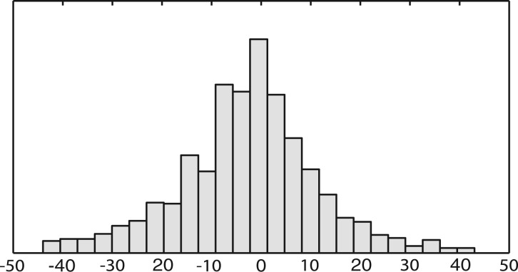
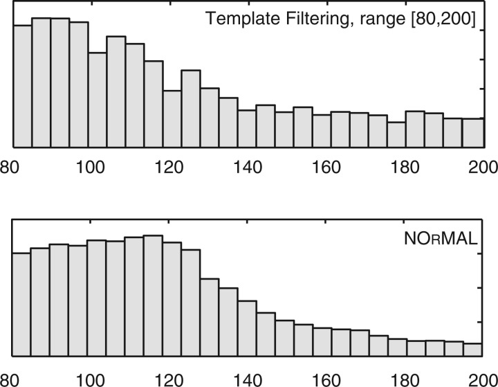
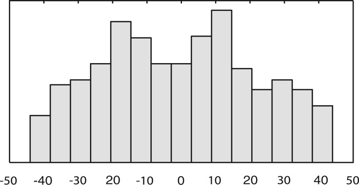
If we compare the distribution of reported nucleosome sizes (Fig. 5), both methods provide consistent results. To compare how reported nucleosomes are related to each other, we performed a matching procedure. We built a bipartite graph, where a node corresponds to a reported nucleosome (each part corresponds to one of the two methods). The bipartite graph is fully connected, and the weight on edge (u,v) is the squared distance between nucleosome u and v: when the distance between u and v exceeded 50 bp, we set the weight to ∞. Then we solved the weighted assignment problem between the two sets using the Hungarian method. The distribution of pairwise distances between matching nucleosomes is shown in Figure 6. Observe that the distribution is a unimodal bell-shaped curve with mean and mode having near zero value. The number of matched (common) nucleosomes is 81.44% of the total: 8.29% and 10.27 are unique to NOrMAL and TF, respectively.

Fig. 5.

Size distribution of reported nucleosomes for S. cerevisiae

Fig. 6.

Distribution of pairwise distances between corresponding nucleosomes reported by TF and NOrMAL for S. cerevisiae

While the dataset for S. cerevisiae is considered to have relatively stable set of nucleosomes (Weiner et al., 2010), the dataset for the human malaria parasite P. falciparum has very dynamic nucleosomes (Ponts et al., 2010). The considered dataset consists of seven time-points (namely, 0, 6, 12, 18, 24, 30 and 36 h), each related to a different stage on the cell cycle (Roch et al., 2003). The experiment assumes that cells are ‘synchronized’ at each time-point, but the synchronization is not perfect due to experimental limitations. As a consequence, we expect a large number to nucleosomes to exhibit a ‘fuzzy’ behavior.

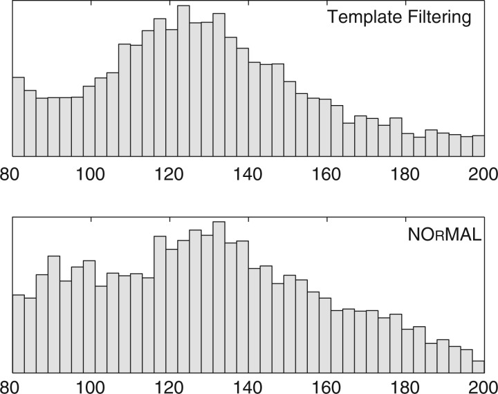
First, we performed nucleosome placement with the same setup as with the yeast dataset. The distribution of fragment sizes is quite different in this case (Fig. 8). NOrMAL reports fragment sizes with a mean value of 105 bp and mode value of about 120 bp, whereas TF reports a distribution with mean and mode of about 84 bp. If we perform the matching of the reported nucleosomes, the distribution of distances is much wider than for yeast (Fig. 7). Now only 50% of all detected nucleosomes are in common between two methods. A total of 32.38 and 17.62% are unique to NOrMAL and TF, respectively. As expected, the disagreement between NOrMAL and TF is much higher on this dataset, due to presence of a much higher fraction of overlapping/fuzzy nucleosomes.

Fig. 8.

Size distribution of reported nucleosomes for P. falciparum (chromosome 1) across all seven time-points

Fig. 7.

Distribution of distances between corresponding nucleosomes reported by TF (range [80,200]) and NOrMAL for P. falciparum (chromosome 1) across all seven time-points

Two examples of the disagreement between TF and NOrMAL are shown in Figure 9. Forward and reverse coverage profiles with extension to 35 bp are shown on top. Nucleosomes are represented by ovals, where the height of each oval represents the confidence score. NOrMAL also reports the variance associated with the left and the right boundary, represented with error bars. In Figure 9 (top), we have labeled corresponding nucleosomes 1–6. Some observations are in order. First, nucleosome 3 is an incarnation of the synthetic example in Figure 4D and E. The coverage profile around coordinate 800 shows two heavily overlapping nucleosomes that should be reported as one ‘fuzzy’ nucleosome. However, TF reports the position of the nucleosome using the stronger pair of forward/reverse peaks and completely ignores the other pair of peaks. As a consequence, the coordinate of the reported nucleosome is shifted compared to the centroid of the four peaks. NOrMAL instead correctly places one nucleosome at the centroid with a relatively high ‘fuzziness’ score. Nucleosome 3 is also quite fuzzy, and it is better placed by NOrMAL. Some disagreement exists on nucleosome 6 as well. The left boundary of that nucleosome detected by TF correspond to a very weak peak. This is due to the fact that TFs placement is based on the correlation score rather than the intensity of the peak. In fairness, both methods assign nucleosome 6 a very low confidence score. Finally, TF detects additional nucleosomes a and b, whereas NOrMAL reports additional nucleosome c. All these nucleosomes have low confidence scores. Our method did not report a and b because it explained the data using fuzzy nucleosome 2. NOrMAL should have merged nucleosome c to nucleosome 1, but because the overlap did not exceed the chosen threshold those two nucleosomes were not merged.

Fig. 9.

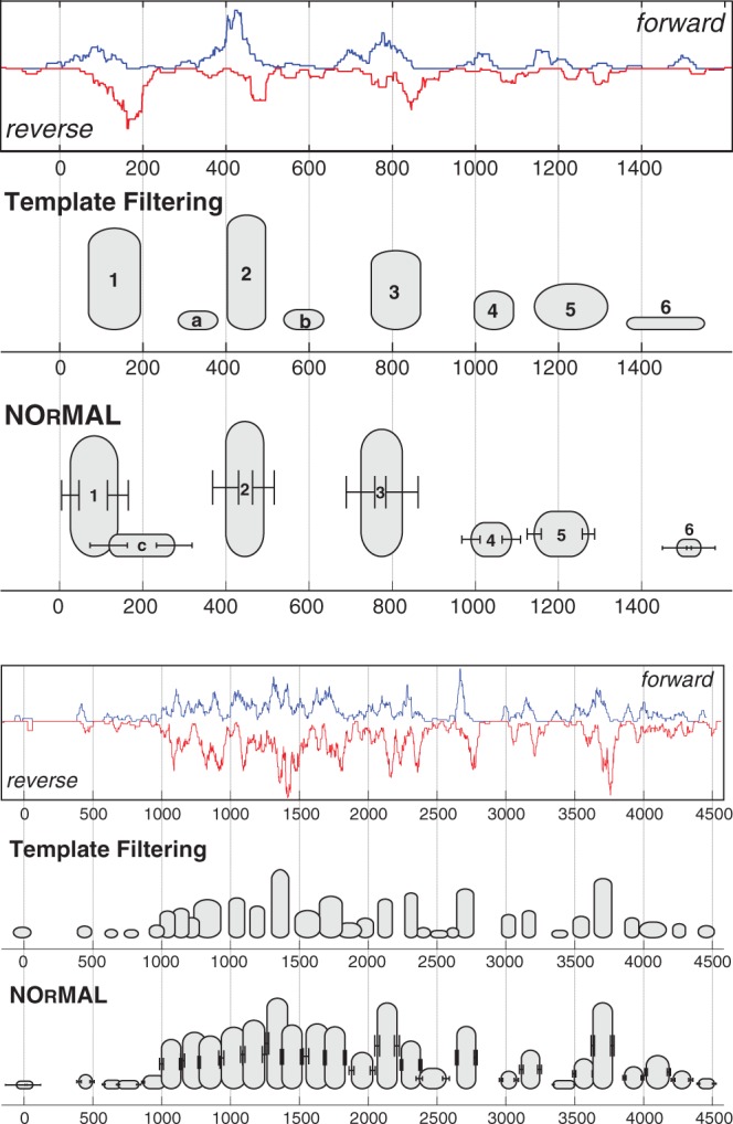
Two examples of nucleosome maps for chromosome 1 of P. falciparum (top: ‘0’ is location 148 500 bp, bottom: ‘0’ is location 111 500 bp): forward and reverse coverage profiles are shown on top; nucleosomes are represented by ovals where the height of each nucleosome represents the confidence score

Figure 9 (bottom) illustrates a more complex example of the coverage profile: even for trained experts placing nucleosomes here would be very challenging. The output of NOrMAL and TF are quite consistent for nucleosomes associated to strong peaks. In the regions with high density of peaks, TF tends to place nucleosomes of small sizes (see also Fig. 10) and pack them as tight as possible according to allowed overlapping threshold.

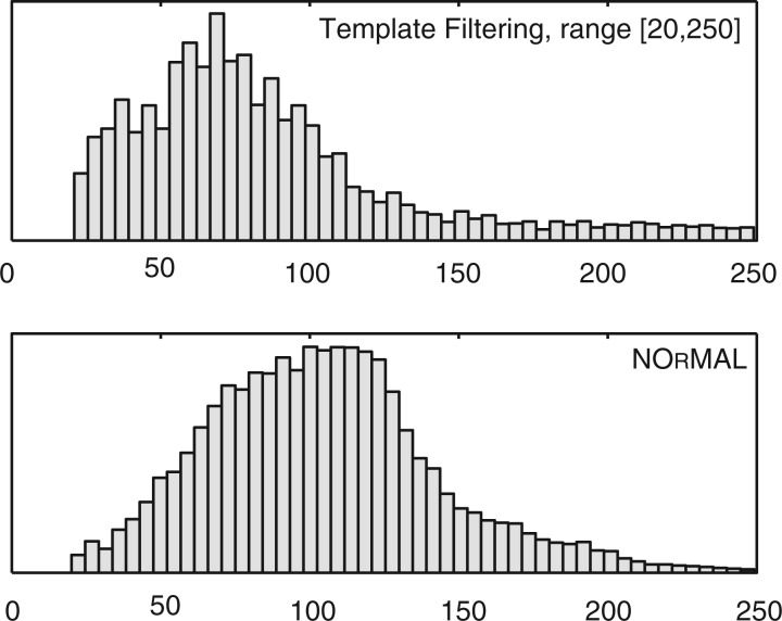
Fig. 10.

Size distribution of reported nucleosomes for P. falciparum (chromosome 1) across all seven time-points

In order to increase the agreement between TF and NOrMAL, we tried to extend the range of nucleosome sizes for TF to [20,250]. The new fragment size distributions are shown on Figure 10. Observe that by comparing Figures 8 and 10, the size distribution for NOrMAL are the same (only truncated in Fig. 8), while the distribution for TF has changed completely, again pointing out how this range parameter can drastically change the results. Using the extended range, TF was allowed to place smaller nucleosomes so the mode and the mean of the size distribution shifted to smaller values. According to the authors of TF, such small nucleosomes can be due to problems in the experimental procedure, namely overexposing the sample to the MNase digestion. However, the gel electrophoresis analysis shows that the expected size of sequenced fragments in our samples after digestion was about 130 bp in length (without adapters). We speculate that TFs approach might have a problem when the range of admissible nucleosome sizes is too wide, and the algorithm confuses boundaries of neighboring nucleosomes.

The number of reported nucleosomes for all time-points is shown in Table 3. Observe that for time-points 0–24 h, the number of nucleosomes reported by NOrMAL is between TF with range [80,200] and [20,250]. However, recall that the extended range [20,250] is likely to be unreliable. For time-point 30 and 36 h, NOrMAL identifies a higher number of nucleosomes. The 30 and 36 h marks correspond to the schizont stage of the P. falciparum life cycle (Roch et al., 2003). During this stage, the parasites divide, the chromatin compacts and a large number of nucleosomes are added.

Table 3.

Number of nucleosomes reported for P. falciparum (chromosome 1) for different time-points (TF, parameter in square brackets is the range of admissible nucleosome sizes, bold numbers indicate the maximum)

Time (h)	TF [80–200]	TF [20–250]	NOrMAL
0	1 720	2 031	1 934
6	1 491	1 826	1 720
12	1 461	2 158	2 043
18	1 185	1 665	1 537
24	1 440	1 910	1 766
30	1 723	2 229	2 443
36	1 701	2 514	2 788

4 CONCLUSION

We described a parametric probabilistic model for nucleosomes positioning framed in the context on a modified Gaussian mixture model. Our method directly addresses the challenges imposed by overlapping and fuzzy nucleosomes, their detection and the inference of their characteristics. We demonstrated with a synthetic example that the current state-of-the-art method does not properly handle complex overlapping configurations. We have also shown that NOrMAL is significantly more robust to user-defined parameters. On real data, our method detects a higher number of nucleosomes. Although our method is currently slower than TF, the processing time is still modest compared to other steps in the sequencing pipeline and we believe the efficiency of NOrMAL can be improved.

REFERENCES

- Albert I., et al. Translational and rotational settings of H2A.Z nucleosomes across theSaccharomyces cerevisiaegenome. Nature. 2007;446:572–576. doi: 10.1038/nature05632. [DOI] [PubMed] [Google Scholar]
- Allan J., et al. Micrococcal nuclease does not substantially bias nucleosome mapping. J. Mol. Biol. 2012;417:152–164. doi: 10.1016/j.jmb.2012.01.043. [DOI] [PMC free article] [PubMed] [Google Scholar]
- Field Y., et al. Distinct modes of regulation by chromatin encoded through nucleosome positioning signals. PLoS Comput. Biol. 2008;4:e1000216. doi: 10.1371/journal.pcbi.1000216. [DOI] [PMC free article] [PubMed] [Google Scholar]
- Field Y., et al. Gene expression divergence in yeast is coupled to evolution of DNA-encoded nucleosome organization. Nat. Genet. 2009;41:438–445. doi: 10.1038/ng.324. [DOI] [PMC free article] [PubMed] [Google Scholar]
- Kaplan N., et al. The DNA-encoded nucleosome organization of a eukaryotic genome. Nature. 2009;458:362–366. doi: 10.1038/nature07667. [DOI] [PMC free article] [PubMed] [Google Scholar]
- Le Roch K.G., et al. Discovery of gene function by expression profiling of the malaria parasite life cycle. Science. 2003;301:1503–8. doi: 10.1126/science.1087025. [DOI] [PubMed] [Google Scholar]
- Mavrich T.N., et al. A barrier nucleosome model for statistical positioning of nucleosomes throughout the yeast genome. Genome Res. 2008a;18:1073–1083. doi: 10.1101/gr.078261.108. [DOI] [PMC free article] [PubMed] [Google Scholar]
- Mavrich T.N., et al. Nucleosome organization in the drosophila genome. Nature. 2008b;453:358–362. doi: 10.1038/nature06929. [DOI] [PMC free article] [PubMed] [Google Scholar]
- Parzen E. On estimation of a probability density function and mode. Ann. Math. Stat. 1962;33:1065–1076. [Google Scholar]
- Ponts N., et al. Nucleosome landscape and control of transcription in the human malaria parasite. Genome Res. 2010;20:228–238. doi: 10.1101/gr.101063.109. [DOI] [PMC free article] [PubMed] [Google Scholar]
- Ponts N., et al. Nucleosome occupancy at transcription start sites in the human malaria parasite: A hard-wired evolution of virulence? Infect. Genet. Evol. 2011;11:716–724. doi: 10.1016/j.meegid.2010.08.002. [DOI] [PMC free article] [PubMed] [Google Scholar]
- Sasaki S., et al. Chromatin-associated periodicity in genetic variation downstream of transcriptional start sites. Science. 2009;323:401–404. doi: 10.1126/science.1163183. [DOI] [PMC free article] [PubMed] [Google Scholar]
- Shivaswamy S., et al. Dynamic remodeling of individual nucleosomes across a eukaryotic genome in response to transcriptional perturbation. Plos Biol. 2008;6:e65. doi: 10.1371/journal.pbio.0060065. [DOI] [PMC free article] [PubMed] [Google Scholar]
- Valouev A., et al. A high-resolution, nucleosome position map ofC. elegansreveals a lack of universal sequence-dictated positioning. Genome Res. 2008;18:1051–1063. doi: 10.1101/gr.076463.108. [DOI] [PMC free article] [PubMed] [Google Scholar]
- Weiner A. High-resolution nucleosome mapping reveals transcription-dependent promoter packaging. Genome Res. 2010;20:90–100. doi: 10.1101/gr.098509.109. [DOI] [PMC free article] [PubMed] [Google Scholar]
- Zaret K. Micrococcal nuclease analysis of chromatin structure. Current Protocols in Molecular Biology. 2005;69:21.1.1–21.1.17. doi: 10.1002/0471142727.mb2101s69. [DOI] [PubMed] [Google Scholar]
- Zhang Z., Pugh B.F. High-Resolution Genome-wide Mapping of the Primary Structure of Chromatin. Cell. 2011;144:175–186. doi: 10.1016/j.cell.2011.01.003. [DOI] [PMC free article] [PubMed] [Google Scholar]