Fast alignment of fragmentation trees

Abstract

Motivation: Mass spectrometry allows sensitive, automated and high-throughput analysis of small molecules such as metabolites. One major bottleneck in metabolomics is the identification of ‘unknown’ small molecules not in any database. Recently, fragmentation tree alignments have been introduced for the automated comparison of the fragmentation patterns of small molecules. Fragmentation pattern similarities are strongly correlated with the chemical similarity of the molecules, and allow us to cluster compounds based solely on their fragmentation patterns.

Results: Aligning fragmentation trees is computationally hard. Nevertheless, we present three exact algorithms for the problem: a dynamic programming (DP) algorithm, a sparse variant of the DP, and an Integer Linear Program (ILP). Evaluation of our methods on three different datasets showed that thousands of alignments can be computed in a matter of minutes using DP, even for ‘challenging’ instances. Running times of the sparse DP were an order of magnitude better than for the classical DP. The ILP was clearly outperformed by both DP approaches. We also found that for both DP algorithms, computing the 1% slowest alignments required as much time as computing the 99% fastest.

Contact: sebastian.boecker@uni-jena.de

1 INTRODUCTION

Metabolomics deals with the identification and quantification of small compounds below 1000 Da, and has received increasing interest during the last years (Last et al., 2007). All organisms, especially plants, fungi and bacteria, synthesize many different metabolites and a large portion of them is still unknown (Fernie et al., 2004). The genome sequence usually does not reveal information about metabolite structure, as it does for protein structure. Newly identified metabolites often serve as leads in drug design (Li and Vederas, 2009; Schmidt et al., 2007), in particular for antibiotics.

For a high-throughput analysis of metabolites and other small molecules, mass spectrometry (MS) is the predominant technology (Cui et al., 2008; Fernie et al., 2004; Last et al., 2007). Nuclear magnetic resonance reveals more information about the analyte, but is inapplicable for high-throughput analysis due to its low sensitivity. MS can be coupled with a separation method (gas chromatography, liquid chromatography or capillary electrophoresis) to analyze complex mixtures like cell extracts (Fiehn, 2008; Halket et al., 2005). To obtain information beyond the compound mass, the analyte is usually fragmented, and fragment masses are recorded. Typically, collision-induced dissociation is combined with liquid chromatography–MS, whereas gas chromatography–MS uses electron impact fragmentation. The first attempt to develop computational methods for analyzing fragmentation spectra of metabolites has been the DENDRAL project in 1965 (Lederberg, 1965). But the project was stopped after it became clear that automated structure elucidation using MS data could not be achieved at that time. Today, data analysis is still the major bottleneck in metabolomics (Neumann and Böcker, 2010). Manual data analysis requires time and deep knowledge of the underlying chemistry (Werner et al., 2008). Due to the limited reproducibility of the data, even library searches are difficult (Oberacher et al., 2009). Additionally, spectral libraries are vastly incomplete. Methods for de novo sequencing of non-ribosomal peptides have recently been developed. But these methods rely on the fact that the analytes are structurally restricted polymers with predictable fragmentation.

When manually analyzing tandem MS spectra, chemists try to annotate fragmentation peaks and identify relations between fragments, resulting in fragmentation pathways. This approach has been automated by Böcker and Rasche (2008). They calculate hypothetical fragmentation trees solely based on the MS data. Fragmentation tree nodes are annotated with the molecular formula of the fragments, whereas edges represent losses. To find a fragmentation tree that shows maximum agreement with the measured data, we search for a tree of maximum edge weight, comparable to prize-collecting Steiner trees (Ljubić et al., 2005). Only lists of common and implausible losses are required as expert knowledge about fragmentation mechanisms. In Rasche et al. (2011), experts evaluated the calculated fragmentation trees and confirmed their excellent quality. Recently, methods to calculate fragmentation trees from multiple MS and gas chromatography–MS data have been developed (Hufsky et al., 2012, manuscript; Scheubert et al., 2011).

MS analysis of similar compounds results in similar fragmentation trees. Rasche et al. (2012) proposed local tree alignments for the automated comparison of fragmentation trees and showed that this method is superior to spectral comparison. Fragmentation tree alignments even allow for inter-dataset comparisons for datasets measured on different instruments (Rasche et al., 2012). A tree alignment may contain matches, mismatches, insertions and deletions, but respects the structure of the two trees. Fragmentation tree similarity is defined via edges (representing losses) and nodes (representing fragments). A local tree alignment contains those parts of the two trees where similar fragmentation cascades occurred.

Tree alignments were introduced by Jiang et al. (1995) and can be applied for RNA secondary structure comparison (Le et al., 1989). RNA structure trees are ordered, that is, the children of any node have a fixed order. In contrast, fragmentation trees are unordered, as there cannot exist any sensible ordering for the sub fragments of some fragment. In this respect, fragmentation trees are more similar to phylogenetic trees than to RNA structure trees. Whereas efficient, polynomial-time algorithms exist for the alignment of ordered trees, the alignment of unordered trees is computationally hard, namely MAX SNP-hard (Jiang et al., 1995). This implies that there exists no Polynomial Time Approximation Scheme (PTAS) for the problem unless P=NP (Arora et al., 1998). In case both trees have fixed maximum out degree, an optimum alignment can be computed via dynamic programming (DP) in polynomial time (Jiang et al., 1995). In comparison, computing the edit distance between two unordered trees remains MAX SNP hard even for bounded degrees (Zhang and Jiang, 1994). An informal algorithm for aligning fragmentation trees was presented by Rasche et al. (2012), and join nodes were introduced to account for missing nodes in one of the trees compared. Missing nodes result from missing peaks in one of the spectra. Rasche et al. (2012) do not give a correctness proof or running time analysis for the algorithm. As related work, we mention the Tree-Constrained Bipartite Matching problem where either a node or any of its descendants may be part of the matching; this problem is also APX-hard (Canzar et al., 2011).

Our contribution: we modify the tree alignment algorithm from Jiang et al. (1995) for edge similarities and local alignments, and analyze its running time. We then show how to integrate join nodes without increasing the worst-case running time. Next, we modify the algorithm to allow for sparse DP, a technique common in RNA folding (Backofen et al., 2011). This does not only decrease the practical memory requirements of the method but, more importantly, also severely decreases running times in practice. Furthermore, we present an Integer Linear Program (ILP) for the fragmentation tree alignment problem, as ILPs often solve NP-hard problems swiftly in practice. We then evaluate all methods on real-world data, and find that the sparse DP approach dominates the classical DP, resulting in an 11-fold speed-up for one dataset. Somewhat unexpectedly, the ILP is clearly outperformed by both DP approaches.

2 ALIGNING FRAGMENTATION TREES

Let T=(V, E) be a tree; the elements of V are called nodes. In the following, we assume all trees to be arboreal, that is, all edges in E are directed away from some root node. By uv, we denote a directed edge from node u to node v. Let p(v) be the parent node of some node v. A fragmentation tree is a tree T=(V, E) together with an edge labeling ℓ : E→. In more detail, nodes V correspond to fragments of a compound, whereas the labels are (neutral or radical) losses: that is, both are molecular formulas over some fixed alphabet of elements (Böcker and Rasche, 2008). Formally, molecular formulas are compomers or multi sets. The children of any node of a fragmentation tree are intrinsically unordered, as there is no sensible way to order the sub fragments of some fragment. In our presentation, we will not consider the molecular formulas of fragments, and concentrate on comparing losses only. As we will see below, comparing fragments instead or comparing both simultaneously requires only minor modifications. See Figure 1 for two examples of fragmentation trees.

Fig. 1.

Optimal fragmentation tree alignment for cystine (11 losses) and methionine (6 losses) from the Orbitrap dataset (a). (b) Fragmentation mass spectra of cystine and methionine. The mass spectra do not share peaks. Molecular structures of cystine (c) and methionine (d). The molecular structures are not known to the alignment method. The alignment detects the common fragmentation path of formic acid–ammonia–ethylene losses and the separate ammonia branch. Additionally, it finds the methylthiol loss, which occurs at a later stage in cystine

We introduce some notation used throughout this article: Let T₁=(V₁, E₁) and T₂=(V₂, E₂) be the two trees we want to align. We sometimes call T₁ the left tree and T₂ the right tree. Let C(v) denote the children (nodes) of any node v in T₁ or T₂. In the following, we usually assume that u is a node of T₁, and v a node of T₂. For i=1, 2, let n_i≔|V_i| be the number of nodes in T_i, and let d_i be the maximum out degree in T_i. These maximum out degrees will be of particular interest to us, as the running time of our DP grows exponentially in d₁, d₂. Let δ=min{d₁, d₂} and Δ=max{d₁, d₂}.

Rasche et al. (2012) introduce a similarity function σ : ×→ℝ for pairs of losses (molecular formulas). We do not repeat the details here, but note that this implies a similarity function σ : E₁×E₂→ℝ between edges of the two trees T₁, T₂ via σ(e₁, e₂)=σ(ℓ(e₁), ℓ(e₂)). They also introduce a similarity function for fragment molecular formulas, which induces a similarity function between nodes of the two trees.

Furthermore, they also extend the definition of tree alignments by introducing a join operator [see Figure 2(b)]: Given a path p₁ in T₁ of length two, let e₁, e₁′ be the edges of p₁. We can assign a loss to p₁ by adding the corresponding losses ℓ(e₁)+ℓ(e₁′)∈. This means taking the sum of the respective compomers or the additive union of the corresponding multisets. We then assign a similarity between p₁ and any edge e₂ of T₂ as σ(p₁, e₂)=σ(ℓ(e₁)+ℓ(e₁′), ℓ(e₂)). Analogously, we can define a similarity for paths of length two in T₂. Obviously, this can be generalized to paths of arbitrary lengths but here, we will limit ourselves to paths of length two. For joining nodes in the alignment, we assume homogeneous join costs: The penalty for joining a node is σ_join≤0, independent of the node or edge that we want to join. Formally, this allows us to focus on the important aspects of our algorithms, and omit some technical details. Practically, we currently see no biologically reasonable way to assign different scores to different join nodes, as these usually correspond to the non-detection of a peak in one of the mass spectra.

Fig. 2.

Two alignments of fragmentation trees based on edge similarities. Nodes represent molecular formulas of the fragments, edges represent molecular formulas of the losses. (a) A gap (−) is introduced for the missing CO loss in the left tree (dashed edge and node). Losses CO and CH₃ are aligned by a mismatch (dotted edges). (b) In the left tree, the fragment after loosing H₃N is missing (dashed edges and node), whereas the fragment after further loss of C₂H₂ is observed. To account for missing fragments, we introduce the join operation. It allows to align the two successive losses H₃N and C₂H₂ in the right tree to a single loss C₂H₅N in the left tree (dotted edges). Fragments may be missing because the corresponding peak was not detected, for example

Let T₁, T₂ be two trees. We define a global alignment of T₁, T₂ as follows (Jiang et al., 1995): is a tree where nodes are labeled with pairs from (V₁∪{−})×(V₂∪{−}). Here, ‘−’ is the gap symbol [see Figure 2(a)]. If we restrict labels of to the first coordinate and contract all edges that end in a node labeled ‘−’, we end up with the tree T₁; if we do the same for the second coordinate, we end up with the tree T₂. (In fact, we have to replace the nodes of the restricted trees by their labels, we omit the simple technical details.) We say that is a local alignment if the trees originating from contracting gap edges are induced subtrees of T₁ and T₂, respectively.

Different from Jiang et al. (1995), we want to score an alignment based on the edges of the two trees. To this end, for any node a of but the root, let e₁(a) be the unique edge in T₁ that ends in the first coordinate of the label of a, and let e₂(a) be the unique edge in T₂ that ends in the second coordinate of the label of a. In case no such edge exists, we assume e₁(a)=‘−’ or e₂(a)=‘−’, respectively. Now, we define the score of as

We define σ(T₁, T₂) as the maximum score of a local alignment of T₁ and T₂.

Scoring node pairs and scoring edge pairs are closely related: We can push an edge score into its end node, or we can pull a node score into its unique incoming edge. The only difference is that the root node is not considered when scoring edge pairs. The two scorings can be combined by introducing a particular root scoring σ^* : V₁×V₂→ℝ for the root nodes of the alignment. In the following, we omit the simple but somewhat tedious details, and simply note that all algorithms presented here work both with node scoring, edge scoring, as well as a combination thereof. A local fragmentation tree alignment for two compounds from the Orbitrap dataset (see Section 6) can be found in Figure 1.

3 DYNAMIC PROGRAMMING

We now present an algorithm to compute optimum fragmentation tree alignments that has reasonable running time in practice. Our algorithm is a modification of an algorithm by Jiang et al. (1995) for computing global alignments of unordered trees. The reason for these algorithms to be swift in practice is that fragmentation trees usually have comparatively small out degree: fragments rarely have more than, say, five child fragments. We can limit the inevitable exponential part of the running time to this out degree.

We use DP to compute the maximal score σ(T₁, T₂) of a local alignment between two trees T₁, T₂. Let S(u, v) be the maximal score of a local alignment of two subtrees of T₁, T₂, where the subtree of T₁ is rooted in u, and the subtree of T₂ is rooted in v. For A⊆C(u) and B⊆C(v), we define S_u,v[A, B] to be the score of an optimal local alignment of subtrees rooted in u and v, respectively, such that maximally the children A of u and B of v are used in the alignment. Clearly, S(u, v)=S_u,v[C(u), C(v)]. Furthermore, we have S_u,v[A, ∅]=S_u,v[∅, B]=0 for all A, B. When all S(u, v) are known, we can compute the maximal score of a local alignment of T₁, T₂ as

(1)

We present a recurrence for the computation of S_u,v[A, B]. We initialize S_u,v[A, B]=0 for A=∅ or B=∅. Recall that T₁ is the left tree and T₂ is the right tree. In the recurrence, we distinguish three cases, namely match (including mismatches), deletion left or deletion right, where the latter two are symmetric (Figure 3). For non-empty sets A⊆C(u) and B⊆C(v) we set

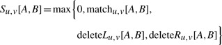where we define

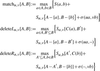(2)

Here, σ(ua, vb) denotes the score of the losses attached to arcs ua and vb, and σ(ua, −), σ(−, vb) accordingly. Recurrence (2) is the obvious modification of the recurrence presented in (Jiang et al., 1995) for global alignments and node similarities.

Fig. 3.

Representation of the match and the deleteL recurrences of the DP algorithm. (a) match_u,v[A, B] is the best score of matching edge ua on edge vb, such that maximally the children A of u and B of v are used. (b) deleteL_u,v[A, B] is the best score for deleting edge ua, such that maximally the children A of u and B of v are used. A subset B′⊆B of the children of v can now be matched to the children of a

Merging two losses in T₁ or T₂ requires two additional symmetric cases, namely join left and join right for merging in tree T₁ or T₂, respectively. To speed up computations, we add an additional prejoin case for nodes that will be joined in the alignment. We set

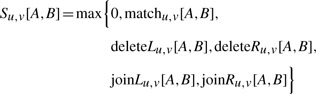(3)

where we define, in addition to (2),

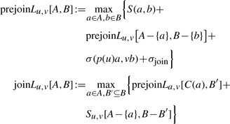(4)

Here, σ(p(u)a, vb) is the score for the combined losses on the path from p(u) to a with the loss of edge vb. Recall that σ_join≤0 is the penalty for joining a node. Again, we initialize joinL_u,v[A, ∅]=joinL_u,v[∅, B]=0 for all A, B. Analogously to (4), we can define recurrences for prejoinR_u,v[A, B] and joinR_u,v[A, B].

For bottom-up DP (Sniedovich, 2006), we have to find an order in which the entries of the DP tables can be filled. Computation of match_u,v[A, B], deleteL_u,v[A, B] and deleteR_u,v[A, B] only accesses entries S_u′,v′[A′, B′], such that u′∈{u}∪C(u) and v′∈{v}∪C(v). By processing nodes in postorder, we ensure that all S_u′,v′[A′, B′] are previously computed for (u′, v′)≠(u, v). For the remaining case, we iterate |A|+|B|=0, 1,…, |C(u)|+|C(v)|. Similar arguments hold for the computation of join and prejoin nodes.

Theorem 1. —

Let T₁=(V₁, E₁) and T₂=(V₂, E₂) be two trees, σ : E₁∪{−}×E₂∪{−}→ℝ a scoring function between edge pairs, and σ_join∈ℝ the penalty for joining a node. For i=1, 2 set n_i≔|V_i|, and let d_i be the maximum out degree in T_i. The maximum score σ(T₁, T₂) of a local alignment of T₁, T₂ can be computed in O(3^Δ · 2^δ · δn₁ n₂) using recurrence (3) and equation (1), where Δ≔max{d₁, d₂} and δ≔min{d₁, d₂}.

The proof of the theorem is based on the following lemma:

Lemma 1. —

Computing S_u,v[A, B] for all A⊆C(u) and B⊆C(v) is possible using recurrence (3) in O(3^d_u · 2^d_v · d_v+2^d_u · 3^d_v · d_u) time, where d_u=|C(u)| and d_v=|C(v)|.

See the Supplementary Material for proofs of Lemma 1 and Theorem 1. Similarly to Theorem 1, we can show that any pairwise tree alignment that does not take joining nodes into account, can also be computed in this time. We leave out the straightforward details.

Theorem 2. —

A pairwise unordered tree alignment (global or local, scoring nodes or edges or both, with similarities or costs) of rooted trees T₁, T₂ can be computed in O(3^Δ · 2^δ · δn₁ n₂) time. Here, n_i is the number of nodes in tree T_i, and d_i is the maximum out degree in T_i, for i=1, 2; furthermore, Δ≔max{d₁, d₂} and δ≔min{d₁, d₂}.

4 SPARSE DYNAMIC PROGRAMMING

Applying the above algorithm to real-world instances of aligning fragmentation trees, one can see that S(u, v)=0 holds for many node pairs u, v. This can be attributed to two factors: First, we are computing local alignments, so we can always choose to end the alignment subtrees in the nodes u, v. Second, there are many different labels found at the edges (or nodes) of a fragmentation tree. A reasonable scoring scheme will assign negative scores to most non-matching edge (or node) labels, so it is rather the exception than the rule that we can find two nodes u, v with S(u, v)>0.

The idea is to ‘sparsify’ our DP tables by storing only those table entries with positive values. Thereby, we face the following fact: If S_u,v[A, B]>0 for A⊆C(u) and B⊆C(v) then S_u,v[A′, B′]>0 holds for all supersets A′, B′ with A⊆A′⊆C(u) and B⊆B′⊆C(v). So, as soon as we have one non-zero entry in the table, then an exponentially large part of the table will be filled with non-zero entries, too.

To negate this rather unfortunate effect, we modify our DP as follows: for A⊆C(u) and B⊆C(v), we define S′_u,v[A, B] to be the score of an optimum local alignment with subtrees rooted in u and v, respectively, such that exactly the children A of u and B of v are used in the local alignment. If no such alignment exists, we set S′_u,v[A, B]=−∞. Then S′_u,v[∅, ∅]=0, but for all A, B ≠ ∅ we have S′_u,v[A, ∅]<0, S′_u,v[∅, B]<0. Clearly,

(5)

We need one more trick in our recurrence: in (2) we have accessed entries S_a,v[C(a), B′] and S_u,b[A′, C(b)], but this is not possible for the table S′ as the optimal alignments might not use all the children of a or b. To this end, we introduce

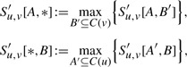for the maximum over all subsets of C(v) or C(u), respectively. For non-empty sets A⊆C(u) and B⊆C(v) we set

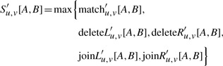(6)

which, compared to (3), misses the lower bound 0 and uses the definitions:

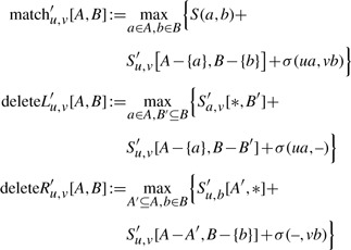(7)

For the further join recurrences, we only concentrate on the left tree. The definition of prejoinL′_u,v[A, *] and the join recurrences at the right tree are analogous.

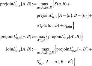(8)

To summarize, the central point is that we do not have to store any entries with S′_u,v[A, B]≤0: such entries will never lead to an optimal alignment, as we are better off removing all nodes A, B, plus everything below these nodes from the alignment. The only exception to this rule is that we store the entry S′_u,v[∅, ∅]=0. Furthermore, we do not have to store entries S′_u,v[A, B] if there exist subsets A′⊆A, B′⊆B with (A′, B′)≠(A, B) such that S′_u,v[A, B]≤S′_u,v[A′, B′]. In this case, we can replace an alignment that uses children A, B of u, v, by an alignment that uses only children A′, B′ and has better or equal score. We say that an entry S′_u,v[A, B] is dominated by entry S′_u,v[A′, B′]. For a scoring scheme that assigns negative scores for non-matching edge (or node) labels, large parts of the tables have negative scores or are dominated by another entry. We do not actually have to forbid that dominated entries are stored, as they do not interfere with our computations; rather, we are free to leave out dominated entries when we encounter them.

The resulting tables S′_u,v are sparsely populated, and for many vertices u, v, there are no entries with S′_u,v[A, B]>0. We can reduce the memory consumption of the method using hash maps instead of arrays. Hash map implementations like Cuckoo hashing (Pagh and Rodler, 2004) or Hopscotch hashing (Herlihy et al., 2008) can carry out all operations in constant (amortized) time. In practice, we find that memory consumption is usually not prohibitive. In this case, we can use lazy arrays that are not allocated until a first entry is stored.

Resolving the recurrences: Now, it is time for our final trick: instead of computing the scores using recurrence (6–8), we apply a successive approximation procedure similar to Dijkstra's Algorithm for shortest paths (Sniedovich, 2006). That is, instead of ‘pulling’ scores from previously calculated entries, we ‘push’ scores from entries that have been finalized. For example, assume that we have finalized the computation of some entry S′_u,v[A, B] for fixed A⊆C(u) and B⊆C(v). Also assume that S′_u,v[A, B]>0 as otherwise, S′_u,v[A, B] is dominated by S′_u,v[∅, ∅]=0. Then, recurrence (7) tells us that we can update other entries of the table accordingly: if S′_u,v[A, B]>S′_u,v[*, B] (which we assume to be incompletely calculated so far) then S′_u,v[*, B] ← S′_u,v[A, B]. Similarly, if S′_u,v[A, B]>S′_u,v[A, *] then S′_u,v[A, *] ← S′_u,v[A, B], and if S′_u,v[A, B]>S(u, v) then S(u, v) ← S′_u,v[A, B]. Regarding the recurrence for match′, we iterate over all a∈C(u)∖A and b∈C(v)∖B: If match′_u,v[A∪{a}, B∪{b}]<S(a,b)+S′_u,v[A, B]+σ(ua, vb) then update it accordingly. If match′_u,v[A∪{a}, B∪{b}]≤match′_u,v[A, B] then the entry match′_u,v[A∪{a}, B∪{b}] is dominated and we can remove it from the hash map.

For all other cases, similar updates can be performed, which we only sketch here: For deleteL′ we iterate over all a∈C(u)∖A and B′⊆C(v)∖B; if deletaL′_u,v[A∪{a}, B∪B′]<S′_a,v[*, B′]+S′_u,v[A, B]+σ(ua, −) then update it accordingly. Updates have to be performed as soon as an entry is finalized, that is, it cannot be changed by any future modifications. Finding finalized entries is similar to the order of computations in the previous section; we omit the technical details.

The above algorithm has exactly the same worst-case running time complexity as the initial recurrence from Section 3. But in practice, we can get even faster, at least in cases where the arrays are very sparse: to this end, finalizing some entry deleteL′_u,v[A, B] triggers updates for all subsets B′⊆C(v)∖B. But only those B′ can lead to relevant updates where S′_a,v[*, B′]>0 holds. Otherwise, the updated entry will be dominated by S′_a,v[*, ∅]=0. If we iterate over the hash map for those B′ with S′_a,v[*, B′]>0 then the worst-case running time increases to O(4^Δ · 2^δ · δn₁ n₂), assuming constant time access to the hash map. However, in practice, running time decreases if the DP tables are sparsely populated. We stress that the sparse DP still guarantees to find the optimal solution.

5 INTEGER LINEAR PROGRAMMING

ILPs are a classical approach for finding exact solutions of computationally hard problems. We now present an ILP for computing a pairwise unordered tree alignment. Again, let T₁=(V₁, E₁), T₂=(V₂, E₂) be the input trees with V₁∩V₂=∅. As the ILP is edge based, we have to introduce some additional notation: Let e∈E_i, i∈{1, 2}, be any edge in one of the two given trees. We denote by (e) the set of edges in the subtree rooted at the head of e, and by (e)≔E_i∖({e}∪(e)) the non-descendant edges of e. For an edge e, we define p(e) to be the parent edge, and p^*(e)≔{p(e), p(p(e)),…} all of its ancestor edges. Finally, (e)≔(p(e))∩(e) is the ‘extended family’ of e, that is, all descendants of e's parent edge, except for e and its descendants.

We start with the ILP without considering the join operation (ILP 1) and use the following binary variables: Iff an edge e′∈(E₁∪E₂) appears in the aligned subtree, we have z_e′=1; iff this edge is aligned to a gap, we have y_e′=1. Finally, iff an edge e∈E₁ is aligned to an edge f∈E₂, we have x_{e,f}=1. The constraints (10) ensure for each edge that we decide whether this edge is used in the alignment and if, how it is aligned. The inequalities (11) ensure that the subgraphs of T₁ (and T₂) are proper trees. Finally, (12) ensure that the obtained alignments are consistent: assume an alignment 〈e,f〉 then we cannot also align a descendant of e with a non-descendant of f and vice versa. The conditional term following the universal quantifier simply avoids redundancy.

ILP 1: —

The ILP for pairwise unordered tree alignment without join operations

(9)

(10)

(11)

(12)

(13)

Based thereon, we can construct an ILP allowing join operations (ILP 2). Therefore, we require additional binary variables x⁽ⁱ⁾_{e,f} (with i∈{1, 2}, e∈E_i, f∈E_3−i), which are 1 iff the joined edges (p(e), e) are aligned with f. Technically, we also require x_{e,f}=1 in such a case. Note that this amount of additional variables is necessary to compose a linear objective function, when the join costs cannot be computed only based on align- and gap costs. Furthermore, we introduce binary variables ϕ_e′, e′∈(E₁∪E₂), which are 1 iff the edge e′ is used as a parent edge within a join (e.g., ϕ_p(e)=1 if the former x⁽ⁱ⁾_{e,f} variable is 1). We use the shorthands σ⁽¹⁾(e,f)≔σ(e+p(e),f)+σ_join−σ(e,f) and σ⁽²⁾(e,f)≔σ(e,f+p(f))+σ_join−σ(e,f) in the objective function.

ILP 2: —

The ILP for pairwise unordered tree alignment including join operations

(14)

(15)

(16)

(17)

(18)

(19)

(20)

(21)

(22)

(23)

(24)

Constraints (15)–(17) are analogous to the former ILP. While (18) guarantees that joins are always separated from each other within an input tree, (19) ensures that at most one joined alignment may occur for any edge. Inequalities (20)–(22) make sure that a parent edge e′ is only marked as a joined parent iff all its aligned children are joined with e′. Finally, (23) guarantees that we do not align two joined edges with each other.

6 EXPERIMENTAL RESULTS

To evaluate our work, we used three different test datasets (Table 1). The Orbitrap dataset (Rasche et al., 2012) contains 97 compounds, measured on a Thermo Scientific Orbitrap XL instrument. The MassBank dataset (Horai et al., 2010) consists of 370 compounds measured on a Waters Q-Tof Premier spectrometer. The Hill dataset consists of 102 compounds measured on a Micromass Q-Tof, published by Hill et al. (2008). We omit the experimental details. Fragmentation trees were computed using ILP as described in Rauf et al. (2012). Self-alignments were excluded from the analysis.

Table 1.

The three datasets used in this study

Characteristics of the datasets	Orbitrap	MassBank	Hill
Number of compounds	97	370	102
Number of non-empty trees	93	343	102
Maximum out degree	7	6	10
Average/median out degreemax	3	2	5
Number of alignments	4 278	58 653	5 151

Fragmentation trees were computed for all compounds. Only non-empty trees were considered for tree alignment. The maximum out degree of a single tree is denoted by out degree_max. Number of alignments is given without self-alignments.

For our evaluations, we use a scoring function very similar to the one from (Rasche et al., 2012), evaluating pairs of losses and pairs of fragments. For losses nl₁, nl₂, we distinguish between size-dependent positive match scores σ(nl, nl)≔5 + number of non-hydrogen atoms and size-dependent negative mismatch scores σ(nl₁, nl₂)≔−5 number of different non-hydrogen atoms. For fragments f₁, f₂, we use size-dependent positive match scores σ(f,f)≔5 + number of non-hydrogen atoms and size-independent negative mismatch scores σ(f₁,f₂)≔−3. We allow insertion/deletions, as well as joining two subsequent losses, both without penalty. The idea behind this ad hoc scoring is to reward or penalize large losses stronger than small losses, whereas non-matching fragments are penalized independent of size. See Rasche et al. (2012) for details.

We implemented the DP algorithms in Java 1.6. For the sparse DP, we used lazy arrays to store the DP tables. We solved the ILP via branch and cut using CPLEX 12.1 in its default settings. Computation was done on two different but comparable computers, namely on a quad-core 2.2 GHz AMD Opteron processor with 5 GB of main memory for the DP algorithms, and on a quad-core Intel Xeon E5520 with 2.27 GHz in 32-bit mode for the ILP, using 2 GB RAM per job. For the DP algorithms, we repeated computations five times, reporting the minimum running time for each instance.

For the Orbitrap and the MassBank dataset, we found that for over 98% of the instances, the running time was in the range of microseconds for both DP algorithms. For these datasets, we only evaluate total running times for all alignments. For MassBank, the classical DP (Section 3) finished in 4.2 s for an all-against-all alignment of 343 trees, whereas sparse DP (Section 4) only required 1.8 s. For Orbitrap, the classical DP finished in 5.4 s for the all-against-all alignment of 93 trees, whereas sparse DP required 0.6 s, a 9-fold speed-up. In contrast, the ILP needed 9.6 min for all alignments in the MassBank datasets and 14.5 min for all alignments in the Orbitrap dataset.

The Hill dataset contains trees with much higher maximum out degree, so we performed a more detailed running time analysis. Classical DP required 13.9 min and sparse DP finished in 1.3 min, an 11-fold speed-up. Running times of the ILP could only be measured without allowing join operations. For 1241 instances, computations run into the memory limitation of 2 GB. For the remaining alignments, the ILP finished in 11.24 h. Hence, we excluded the ILP from our detailed analysis. To get an overview of the differences in the running times between hard and easy alignments, we sorted the instances by their running times in increasing order. This was done separately for each algorithm. See Figure 4 (top) and Table 2. For both algorithms, we found that the 99% fastest alignments need nearly as much computing time as the remaining 1% slowest alignments. We further sorted all instances by the running time of the classical DP (see again Figure 4). We found that for every instance, sparse DP requires less time than the classical DP.

Fig. 4.

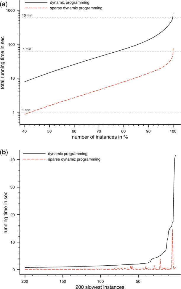
Running times for the Hill dataset with 5151 individual alignments. (a) Total running times when instances are sorted by individual running times. For any fraction x%, we calculate the total running time of the x%, instances for which the alignment was computed faster than for any of the remaining instances. For example at 50% one can find the running time that was needed to compute the 50% fastest instances. For each algorithm, instances were sorted separately. Note the logarithmic y-axis. (b) Individual running times for the 200 slowest instances of the classical DP algorithm. Instances are sorted by their running time for the classical DP algorithm. One can see that running times of the classical DP are outperformed by that of the sparse DP

Table 2.

Running times for the Hill dataset

Algorithm	All	90% fastest	99% fastest	1% slowest
DP	833.3 s	133.5 s (16.0%)	437.9 s (52.6%)	395.4 s (47.4%)
Sparse DP	75.3 s	13.9 s (18.5%)	33.9 s (45.0%)	41.4 s (55.0%)
Speed up	11-fold	10-fold	13-fold	10-fold

We report running times in seconds and as fractions of the total running time for all instances (5151 alignments). We also report running time for the 90 and 99% fastest and for the 1% slowest alignments. For both algorithms, instances were sorted separately.

7 CONCLUSION

Fragmentation trees are a tool to overcome the limitations of spectral library search, as they, for the first time, enable us to retrieve not only exact hits, but also similar compounds from a spectral database. But performing the workflows proposed by Rasche et al. (2012) on a large database requires tree alignments to be executed extremely fast. In this article, we have presented three exact algorithms for the alignment of fragmentation trees. We find that the sparse DP approach dominates the classical DP, resulting in an 11-fold speed-up for one dataset. ILPs have an excellent record of providing fast algorithms for NP-hard problems. Thus, it is rather unexpected that, for the problem discussed here, the ILP is usually clearly outperformed by both DP approaches; still, it has the potential to solve those instances that are ‘hard’ for DP-based algorithms. Also, in such cases we may use the ILP as a heuristic, solving only its LP relaxation and applying some integer rounding algorithm, many of which are standard in state-of-the-art ILP solvers.

When larger datasets become available, we expect the total running time of an all-against-all alignment to increase more than quadratic with dataset size: We have shown above that a large fraction of the total running time stems from a few ‘hard’ alignments which, in turn, correspond to a few trees in the dataset that are large and, in particular, have high out degrees. We conjecture that for larger datasets, the running time spent on computing the 99% fastest alignments will be significantly smaller than the running time spent on the 1% slowest alignments. Here, even faster methods for computing fragmentation tree alignments are sought. We will evaluate whether our ILP is capable of solving these ‘hard’ instances faster than a DP-based approach, as its running time is not directly dependent on the out degree of the trees.

We have put particular focus on fragmentation trees that are hard to align, namely large trees with high out degrees. Small trees with low out degree seem to be less interesting since they often belong to small compounds (<300 Da). Often, these compounds are ‘knowns’ (that is, reference measurements of the compound can be found in a spectral library) and can be identified by spectral comparison. Also, small fragmentation trees contain less information for, say, classifying an unknown compound. Nevertheless, we believe that we can also speed up alignments when one of the fragmentation trees is relatively small: this may be achieved using some preprocessing for small trees with, say, less than four losses.

We conjecture that running time of the DP (Theorems 1 and 2) can be improved to O(2^d₁+d₂ · poly (d₁, d₂)n₁ n₂) using the Möbius transform (Björklund et al., 2007), but this appears to be of theoretical interest only.

In our evaluations, we have used a scoring function similar to the one by Rasche et al. (2012). Both scorings lack any statistical explanation and should be refined in the future using, say, log odds scores. Also, the effect of merging two or possibly even more nodes has to be investigated. Both questions were beyond the scope of this work. Another interesting question is whether polynomial-time methods for tree alignment of unordered trees, such as the constrained tree edit distance (Zhang, 1996), can be used for aligning fragmentation trees: whereas the restrictions imposed by Zhang (1996) have no sensible interpretation in the context of fragmentation trees, quality of results may still be sufficient for certain applications.

Aligning fragmentation trees allows for an automated classification of unknown compounds into compound classes. Thus, large-scale compound screens can easily be searched for compounds of interest. This may be useful in the search for signaling molecules, biomarkers, or novel drugs and the identification of illegal drugs or toxins. In conjunction with other methods from systems biology, the concept can help to identify new metabolic pathways based on tandem MS experiments.

REFERENCES

- Arora S., et al. Proof verification and the hardness of approximation problems. J. ACM. 1998;45:501–555. [Google Scholar]
- Backofen R., et al. Sparse RNA folding: time and space efficient algorithms. J. Discrete Algorithms. 2011;9:12–31. [Google Scholar]
- Björklund A., et al. Proceedings of ACM Symposium on Theory of Computing (STOC 2007) New York: ACM Press; 2007. Fourier meets Möbius: fast subset convolution; pp. 67–74. [Google Scholar]
- Böcker S., Rasche F. Towards de novo identification of metabolites by analyzing tandem mass spectra. Bioinformatics. 2008;24:I49–I55. doi: 10.1093/bioinformatics/btn270. [Proceedings of European Conference on Computational Biology(ECCB 2008)] [DOI] [PubMed] [Google Scholar]
- Canzar S., et al. Proceedings of International Conference on Automata, Languages and Programming (ICALP 2011) Vol. 6755. Berlin: Springer; 2011. On tree-constrained matchings and generalizations; pp. 98–109. [Google Scholar]
- Cui Q., et al. Metabolite identification via the Madison Metabolomics Consortium Database. Nat. Biotechnol. 2008;26:162–164. doi: 10.1038/nbt0208-162. [DOI] [PubMed] [Google Scholar]
- Fernie A.R., et al. Metabolite profiling: from diagnostics to systems biology. Nat. Rev. Mol. Cell Biol. 2004;5:763–769. doi: 10.1038/nrm1451. [DOI] [PubMed] [Google Scholar]
- Fiehn O. Extending the breadth of metabolite profiling by gas chromatography coupled to mass spectrometry. Trends Analyt. Chem. 2008;27:261–269. doi: 10.1016/j.trac.2008.01.007. [DOI] [PMC free article] [PubMed] [Google Scholar]
- Halket J.M., et al. Chemical derivatization and mass spectral libraries in metabolic profiling by GC/MS and LC/MS/MS. J. Exp. Bot. 2005;56:219–243. doi: 10.1093/jxb/eri069. [DOI] [PubMed] [Google Scholar]
- Herlihy M., et al. Proceedings of Symposium on Distributed Computing (DISC 2008) Vol. 5218. Berlin: Springer; 2008. Hopscotch hashing; pp. 350–364. [Google Scholar]
- Hill D.W., et al. Mass spectral metabonomics beyond elemental formula: chemical database querying by matching experimental with computational fragmentation spectra. Anal. Chem. 2008;80:5574–5582. doi: 10.1021/ac800548g. [DOI] [PubMed] [Google Scholar]
- Horai H., et al. MassBank: a public repository for sharing mass spectral data for life sciences. J. Mass Spectrom. 2010;45:703–714. doi: 10.1002/jms.1777. [DOI] [PubMed] [Google Scholar]
- Jiang T., et al. Alignment of trees: an alternative to tree edit. Theor. Comput. Sci. 1995;143:137–148. [Google Scholar]
- Last R.L., et al. Towards the plant metabolome and beyond. Nat. Rev. Mol. Cell Biol. 2007;8:167–174. doi: 10.1038/nrm2098. [DOI] [PubMed] [Google Scholar]
- Lederberg J. Topological mapping of organic molecules. Proc. Natl. Acad. Sci. USA. 1965;53:134–139. doi: 10.1073/pnas.53.1.134. [DOI] [PMC free article] [PubMed] [Google Scholar]
- Le S.Y., et al. Tree graphs of RNA secondary structures and their comparisons. Comput. Biomed. Res. 1989;22:461–473. doi: 10.1016/0010-4809(89)90039-6. [DOI] [PubMed] [Google Scholar]
- Li J.W.-H., Vederas J.C. Drug discovery and natural products: end of an era or an endless frontier? Science. 2009;325:161–165. doi: 10.1126/science.1168243. [DOI] [PubMed] [Google Scholar]
- Ljubić I., et al. Proceedings of Algorithm Engineering and Experiments (ALENEX 2005) SIAM; 2005. Solving the prize-collecting steiner tree problem to optimality; pp. 68–76. [Google Scholar]
- Neumann S., Böcker S. Computational mass spectrometry for metabolomics – a review. Anal. Bioanal. Chem. 2010;398:2779–2788. doi: 10.1007/s00216-010-4142-5. [DOI] [PubMed] [Google Scholar]
- Oberacher H., et al. On the inter-instrument and inter-laboratory transferability of a tandem mass spectral reference library: 1. results of an Austrian multicenter study. J. Mass Spectrom. 2009;44:485–493. doi: 10.1002/jms.1545. [DOI] [PubMed] [Google Scholar]
- Pagh R., Rodler F.F. Cuckoo hashing. J. Algorithms. 2004;51:122–144. [Google Scholar]
- Rasche F., et al. Computing fragmentation trees from tandem mass spectrometry data. Anal. Chem. 2011;83:1243–1251. doi: 10.1021/ac101825k. [DOI] [PubMed] [Google Scholar]
- Rasche F., et al. Identifying the unknowns by aligning fragmentation trees. Anal. Chem. 2012;84:3417–3426. doi: 10.1021/ac300304u. [DOI] [PubMed] [Google Scholar]
- Rauf I., et al. Proceedings of Research in Computational Molecular Biology (RECOMB 2012). Vol. 7262. Berlin: Springer; 2012. Finding maximum colorful subtrees in practice; pp. 213–223. [DOI] [PubMed] [Google Scholar]
- Scheubert K., et al. Computing fragmentation trees from metabolite multiple mass spectrometry data. Proceedings of Research in Computational Molecular Biology (RECOMB 2011) 2011;6577:377–391. doi: 10.1089/cmb.2011.0168. [DOI] [PubMed] [Google Scholar]
- Schmidt B.M., et al. Revisiting the ancient concept of botanical therapeutics. Nat. Chem. Biol. 2007;3:360–366. doi: 10.1038/nchembio0707-360. [DOI] [PubMed] [Google Scholar]
- Sniedovich M. Dijkstra's algorithm revisited: the dynamic programming connexion. Control Cybern. 2006;35:599–620. [Google Scholar]
- Werner E., et al. Mass spectrometry for the identification of the discriminating signals from metabolomics: current status and future trends. J. Chromatogr. B. 2008;871:143–163. doi: 10.1016/j.jchromb.2008.07.004. [DOI] [PubMed] [Google Scholar]
- Zhang K., Jiang T. Some MAX SNP-hard results concerning unordered labeled trees. Inf. Process. Lett. 1994;49:249–254. [Google Scholar]
- Zhang K. A constrained edit distance between unordered labeled trees. Algorithmica. 1996;15:205–222. [Google Scholar]
Associated Data
This section collects any data citations, data availability statements, or supplementary materials included in this article.