Improved synapse detection for mGRASP-assisted brain connectivity mapping

Abstract

Motivation: A new technique, mammalian green fluorescence protein (GFP) reconstitution across synaptic partners (mGRASP), enables mapping mammalian synaptic connectivity with light microscopy. To characterize the locations and distribution of synapses in complex neuronal networks visualized by mGRASP, it is essential to detect mGRASP fluorescence signals with high accuracy.

Results: We developed a fully automatic method for detecting mGRASP-labeled synapse puncta. By modeling each punctum as a Gaussian distribution, our method enables accurate detection even when puncta of varying size and shape partially overlap. The method consists of three stages: blob detection by global thresholding; blob separation by watershed; and punctum modeling by a variational Bayesian Gaussian mixture models. Extensive testing shows that the three-stage method improved detection accuracy markedly, and especially reduces under-segmentation. The method provides a goodness-of-fit score for each detected punctum, allowing efficient error detection. We applied this advantage to also develop an efficient interactive method for correcting errors.

Availability: The software is available on http://jinny.kist.re.kr

Contact: tingzhao@gmail.com; kimj@kist.re.kr

1 INTRODUCTION

An important challenge in neuroscience is to map the synaptic connectivity of neuronal networks in mammalian brains. Among advanced technologies for mapping connectivity, the fluorescence-based mGRASP (Kim et al., 2012) stands as a markedly powerful tool for comprehensive studies of synaptic circuits in mammalian brains. The mGRASP technique is based on fluorescence that is reconstituted when two non-fluorescent split GFP fragments targeted to the synaptic membranes in two separate neuronal populations are closely opposed across the synaptic cleft; thus, fluorescence uniquely indicates a synapse. Computational methods including image stitch, neuron reconstruction and synapse detection have been applied successfully to investigate the locations and distributions of synapses in dendritic compartments and in neurons labeled with mGRASP. In our previous study, computational analysis for synapse detection achieved 93% accuracy. Here we introduce optimizations to improve synapse detection and other tasks.

Detecting mGRASP-labeled synapses is complicated by the low signal-to-noise ratios of the original images, the variety of the sizes and shapes of fluorescent puncta, and signal overlap from neighboring puncta (Fig. 1). To overcome these difficulties, we previously applied a method based on Gaussian template matching followed by blob merging (Kim et al., 2012). But, lacking a splitting procedure, this method frequently suffered from under-segmentation, which is the error of counting multiple puncta as one.

Fig. 1.

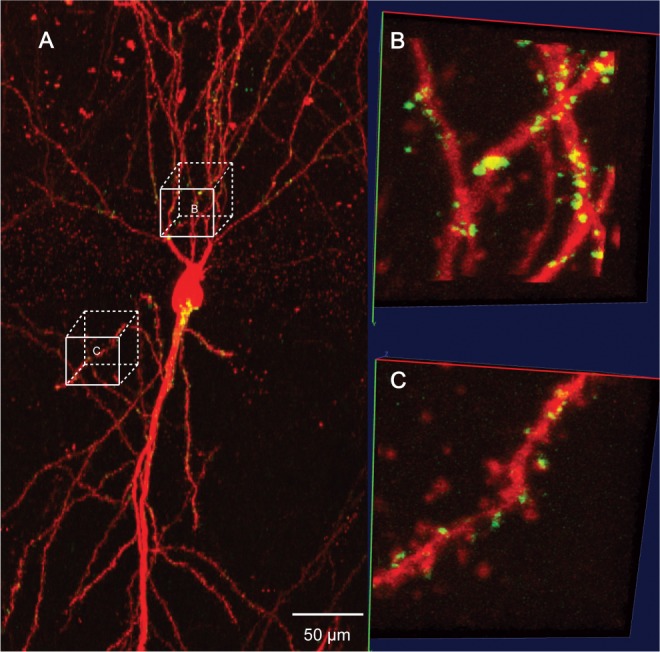
Synapses visualized by mGRASP in a mouse hippocampal CA1 neuron. (A) Merged images show neuronal dendrites in red and mGRASP-labeled synapse puncta in green. (B and C) Zoomed images of two selected areas. Image size of each area is 128×128×99 voxels (corresponding to 13.3 μm × 13.3 μm × 49.5 μm)

Although no other method had been developed specifically for punctum detection in mGRASP images, the problem is closely related to fluorescent particle detection (e.g. GFP-labeled peroxisomes and GLUT4), for which several methods have been published (Bonneau et al., 2005; Mashanov and Molloy, 2007; Sage et al., 2005; Smal et al., 2010). However, most of these methods are not suitable for mGRASP-labeled punctum detection because they cannot accommodate particles featuring a wide range of sizes, irregular shapes and degrees of overlap or they are not readily extended into three dimensions. For example, (Smal et al., 2010) evaluated several 2D particle detection methods and found that multiscale variance-stabilizing transform (MSVST) (Zhang et al., 2007) and h-dome transform (Smal et al., 2008) based methods offered the best performance among unsupervised methods. However, both these methods assume that the particles are well separated. MSVST takes any connected foreground feature as a particle without providing any splitting correction, and h-dome based method treats foreground clusters as noise. Neither method provides a solution to the problem of puncta overlap. The review also introduced two supervised methods, one of which was originally reported in (Jiang et al., 2007). But it is not straightforward to generalize the 2D edge features used in the methods to 3D. In particular, we found it impractical to design a set of template features for our data and to build a sufficiently large training set, both of which are necessary for any supervised method.

A more promising category of method includes those using mixture models, which estimate the shapes, sizes and locations of particles from a blob in one framework. For example, (Thomann et al., 2002) and (Jaqaman et al., 2008) used the mixture of point spread functions to fit clustered particles. (Zhao and Murphy, 2007) employed a Gaussian mixture models (GMMs) to detect protein particles in 2D images. Later this method was extended to 3D by (Peng and Murphy, 2011). However, these methods have a major disadvantage. Since the number of particles is unknown, it is necessary to fit every possible mixture model to the data and then determine the best fit with minimal model complexity. Since this fitting problem is highly non-linear, finding good initial parameters is crucial to the final result. However, for synapse puncta these parameters can be hard to choose because their size is uncertain. Also, these methods lack post-processing for the mixture model, a step necessary for puncta detection since puncta can have irregular shapes and GMMs are sensitive to outlier data.

Other related methods are those used for DAPI-labeled nuclei segmentation, in which a splitting procedure is often necessary (Lin et al., 2003). One of the most impressive nuclei segmentation methods was developed by (Al-Kofahi et al., 2010), who used watershed techniques to separate clustered nuclei and then applied graph cuts to refine the results.

Here we introduce a new method based on a splitting strategy using a marker-controlled watershed approach and a variational Bayesian Gaussian mixture models (VBGMMs) to accurately detect mGRASP-labeled synapses of variable sizes and shapes. Watershed is used for separating connected blobs by distinguishing their centers, and VBGMMs are then used for learning mixture models directly from the image data rather than requiring many initial parameters and an estimate of component number. Following VBGMMs, we implement an effective mean-shift and merge post-processing to further refine the mixture models. We compare our method to others, including the method in (Al-Kofahi et al., 2010), by testing them on a large set of mGRASP data. The results show that our method outperforms other tested methods and markedly improves detection accuracy compared with our previous method.

2 APPROACH

Our main challenge was to correctly separate clustered puncta of mGRASP-labeled synapses of variable sizes and shapes. The two main features of puncta used by our detection algorithm are a clear bright center and a convex shape; these features are also important for a human inspecting these images. Our detection algorithm follows a three stage process. The first stage is to use thresholding to separate the image's foreground voxels from background voxels. Foreground voxels form many clusters. In the second stage, centers of these clusters are marked and then a marker-controlled watershed is utilized to separate them. In the third stage, to detect the correct number and locations of puncta automatically, we use a variational bayesian mixture of gaussians followed by mean-shift to refine detection. For numeric stability, we set a global size threshold N_threshold. In any stage, if the voxel number of a separated part is smaller than N_threshold, this part is treated as a punctum and will not be separated further. N_threshold is set to 20 in the example shown here. Figure 2 shows a flowchart illustrating the main steps of our method.

Fig. 2.

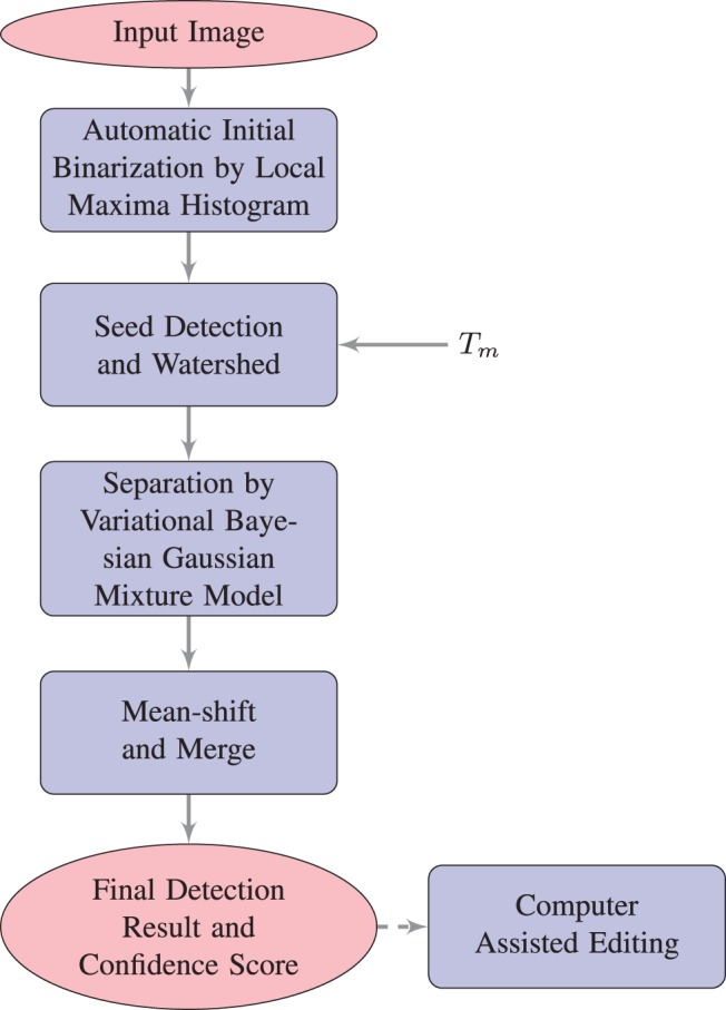
Flow chart outlining the main steps of the proposed puncta detection algorithm

3 METHODS

3.1 Automatic image binarization

The first step is to identify foreground voxels that correspond to fluorescence signals of mGRASP-labeled synapses. We employed a global thresholding method that has been successfully used to extract neurons from light microscope images (Xie et al., 2011; Zhao et al., 2011). In brief, the method takes advantage of the fact that most local maximal regions in a microscope image are background noise. We found that a good threshold turned out to be the transition point of the normalized histogram of local maxima. As shown in Figure 3, from the histogram h where h(i) is the number of local maximum voxels that have the intensity i, we first obtain i_max=argmax_i h(i), the intensity value that has the highest frequency, and i_min=argmin_i h(i), the intensity with the lowest frequency min h(i). We then normalize the histogram as

(1)

It can be shown that T=argmin_i(i−i_max+h_r(i)) is the transition point (Xie et al., 2011), which is also taken as the global threshold to separate the foreground and background of the image.

Fig. 3.

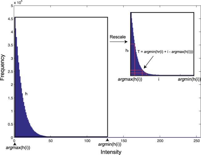
The method of finding a global intensity threshold. The original histogram of local maxima h is obtained by counting voxels in local maximal regions. The normalization rescales the histogram h to h_r by linearly mapping [min h(i), max h(i)] to range [0, argmin_i h(i)−argmax_i h(i)]. The threshold is argmin_i(h_r(i)+i−argmax_i h(i))

3.2 Marker-controlled watershed segmentation

Binarization of an image results in many isolated blobs of connected foreground voxels. There can be one or more puncta in each blob, and the goal of this stage is to identify individual puncta blob by blob. This task is similar to separating touching objects, which is a classical application of the watershed algorithm. In practice, however, the original watershed method tends to generate uncorrectable over-segmentation in a noisy image. One common solution to this problem is to use a marker-controlled version of watershed, which sets a size threshold for adding a ‘catchment basin’ (Vincent, 1993; Yang et al., 2006). Similar to any other watershed method, the marker-controlled watershed starts checking voxels progressively from the highest or lowest gray level, depending upon whether region borders are darker or brighter than region centers. In our case the process starts from the highest gray level because puncta usually have bright centers. At each gray level, a blob is dissected into connected components of voxels with intensities higher than the gray level. When a component contains only one previously defined marker, all voxels will be assigned to that marker; when a component contains more than one marker, any unmarked voxel is assigned to its closest marker. A new marker is added when a component contains no pre-defined marker and the size of a component exceeds the threshold T_m. High T_m value can suppress local maxima caused by noise, thus preventing over-segmentation. For our data, we choose T_m=6. After the watershed process, every voxel of a blob is assigned to one of the markers. Figure 4C shows the result of watershed separating for the example image. It misses one punctum in Part 3 because its signal is weak and the center of the punctum is unclear.

Fig. 4.

Key steps of the proposed puncta detection method. (A) One blob after automatic binarization shown as a maximum intensity projection. (B) 3D view of the blob. (C) The color-coded result of marker-controlled watershed separation, which produced three parts. (D) Each part is passed to the mean-shift regulated VBGMMs. Final detection result contains four puncta. (E) Detailed steps of mean-shift regulated VBGMMs for three watershed separated parts. Blue circles represent data points projected to x–y plane. Ellipsoids are 95% confidence interval Gaussian components in each step

3.3 Mean-shift regulated VBGMMs

Since a punctum is assumed to have a bright center and a convex shape, it can be modeled as a 3D Gaussian distribution. As a result, any blob that has one or more puncta can be modeled as mixture of Gaussians. The data for fitting GMMs at this stage are taken from the previous watershed segmentation. We denote the observed dataset by X={x₁,…, x_N}, where x_n=(x_n, y_n, z_n) for n=1,…, N are the coordinates of the n-th voxel of the component. The intensity I={i₁,…, i_N} where i_n is the intensity of x_n serves as weight value for fitting; that is, we can assume that there are a total of M=∑_n=1^N i_n samples, among which the position x_n is observed i_n times. So the observations can be expanded to (x_j1,…, x_jM), which contains all the duplicates of the voxels. For each observation x_jm we determine a corresponding latent variable z_m comprising a 1-of-K binary vector with elements z_mk for k=1,…, K, where K is the number of Gaussian components. The expectation-maximization (EM) algorithm is often used to estimate model parameters of GMM by maximizing likelihood. The number of Gaussian components, however, has to be given as a known parameter when using an EM procedure. As K is unknown in our case, instead, we would need to analyze the dataset for all possible K values and then use Akaike information criterion (AIC) or Bayesian information criterion (BIC) to compensate for the over-fitting of complex models. This is computationally inefficient. We found an alternative, better, way is to use a fully Bayesian approach based on variational inference that can optimize the trade-off between model complexity and goodness of fit at the same time (Attias, 2000; Bishop, 2006). We adopted this method by adding data weights {i_n|n=1,…, N} to make it better suited for our problem. Given the mixing coefficient π for each Gaussian component, the conditional distribution of the latent class variable Z={z₁,…, z_M} is

(2)

The distribution of the observed data vectors conditioned on the latent variables and the component parameters is

(3)

where μ and Λ are the mean vector and precision matrix. The prior distribution for mixing coefficients π is assumed to be a symmetric Dirichlet distribution

(4)

The mean and precision matrix of each Gaussian component are governed by the Gaussian-Wishart prior

(5)

By assuming that the variational posterior distribution can factorize between latent variables and parameters:

(6)

it can be optimized by repeating two steps, the expectation (E) step and the maximization (M) steps. In the E step, the model parameters are fixed. Current distributions are used to get the responsibility value 𝔼[z_mk], which is the k-th component's contribution to the data point x_jm. Let

(7)

and

(8)

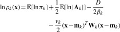
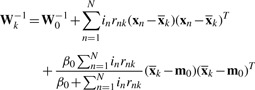
where D=3 is the dimensionality of the data variable x. β_k and v_k are two parameters of prior distributions and updated in the M step. 𝔼[lnπ_k] and 𝔼[ln |Λ_k|] can be calculated by using the Dirichlet and Wishart distribution. Then we have . Since the responsibility value is only related to data position, we can only caculate responsibility for each voxel rather than all duplicated data points. The overall contribution of the k-th component to the data point x_n is i_nr_nk. In the M step, variational distribution parameters are updated based on the fixed responsibility. Define

(9)

We can get the updated variational posterior distributions of π, μ_k and Λ_k as

(10)

(11)

where

(12)

(13)

(14)

(15)

(16)

After convergence, only components that take responsibility for explaining the data points ‘survive’, and those with low responsibility values (∑_n=1^N i_n r_nk) are removed.

Although VBGMMs nicely solve the model selection problem, it requires specifying a proper initial value K₀, which should be the upper bound of the actual number of puncta. For a non-saturated watershed component, we set K₀ as the number of local maximal regions. When the intensity of the component is highly saturated, we use a 2D Euclidean distance map to estimate K₀ instead. To build the distance map, we first binarize the maximum intensity projection (on the x–y plane) of the target component by setting all saturated voxels to 1 and other voxels to 0. The distance map is built upon the foreground of the binary image. We set K as the number of local maxima in the distance map plus the number of non-saturated local maxima in the component. Since bayesian clustering using mixture of Gaussian components is sensitive to outliers and noise (Svensén and Bishop, 2005), both of which can lead to over-estimating the number of components, it is necessary to provide a merging procedure to check whether some components actually belong to the same punctum and, if they do, to merge them. In this procedure, the center m_k of the k-th Gaussian component is readjusted by the mean-shift algorithm, an efficient procedure for locating the nearest stationary point of the underlying density function. By using mean-shift, we can move Gaussian components disturbed by outliers and noise to the desired locations. We can then merge the adjusted components according to their degree of overlap. The mean-shift radius R_k is defined as the semi-minor axis length of the x–y projection of the Gaussian component within its 90% confidence interval. It can be calculated as follows

(17)

where μ_1/2(λ_i) is the median eigenvalue of the covariance matrix of the corresponding Gaussian component and p_conf=0.9 defines the confidence region for its projection. Figure 4E and Figure 5 shows the process of VBGMM fitting, mean-shift and merging. The initial K in Figure 5 is 12, which gives 12 Gaussians in a GMM (Figure 5B), and after the EM steps, only three components remain. The second column of Figure 4E shows the noise sensitivity of GMMs. Since some Gaussian components are fit only to a small number of data points and the number of components is overestimated, they are then fed into the merging procedure. Figure 5D and the third column of Figure 4E show the result of the mean-shift process, where all components were moved to the center of puncta. After that, we merge any pair of Gaussian components if either of their x–y projections have 80% overlap with the other. Figure 5E and last column of Figure 4E show the final results of merging.

Fig. 5.

Illustrating typical mean-shift regulated vbgmm steps. (A) 3D image of one punctum. (B) twelve local maxima voxels are detected, therefore K=12. (C) After VBGMM convergence, three components left. (D) Adjust each component using mean-shift. (E) Final merged result

3.4 Proof-Editing

Although automated detection can provide reasonably accurate results, proof-editing is needed for correcting detection errors in order to avoid drawing misleading conclusions, as can occur in some other bioimage analysis tasks (Peng et al., 2011). Nevertheless, it is very time consuming to scan the whole image visually to search for detection errors because large images may contain thousands of puncta. Therefore, it would be very helpful for an algorithm to provide a detection score for each punctum to estimate the likelihood a given detection is wrong. With such a score, we can significantly improve the efficiency of proof-editing by presenting puncta in the order of their scores or with visual hints of the scores. Another advantage of our method is that it allows calculating the fitting score, e.g. the Pearson's correlation coefficient, between the signal of a punctum and its Gaussian model. The lower this confidence score, the more likely the detection is in error. Low scores can be spotted easily with a colormap as shown in Figure 6B. The punctum with the lowest score in the image is marked by an arrow, and it is indeed an under-segmentation error (Figure 6B).

Fig. 6.

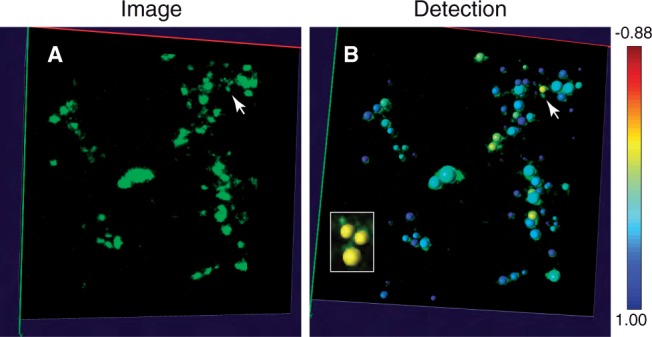
Detection confidence score of puncta for two sample image areas, where the scores are shown as colormap. Image size of each area is 128×128×99 voxels (corresponding to 13.3 μm × 13.3 μm × 49.5 μm). The lower the score (yellow), the more likely the detection error is. (A) Images with green puncta. (B) Confidence score for every punctum. Lowest score is marked by arrow. The marked puncta is clearly under-segmented. After user input the actual puncta number which is 3 and run the EM GMM split, the result becomes correct as shown in the small cropped image

The score and colormap can guide users to find the most problematic regions quickly. After errors are located, they can be corrected using computer-assisted manual editing. Two types of errors can occur. The first is over-segmentation that can be corrected by merging neighboring puncta with one mouse click. The second type is under-segmentation that can be corrected with a splitting procedure carried out by computer after the user specifies that blob to split and how many puncta should result. Here we use GMMs again to split any under-segmented blob. An example of correcting under-segmentation is shown in Figure 6B.

4 EXPERIMENTAL RESULTS

The mGRASP-labeled synapse data used for testing our method were acquired under a Zeiss 710 confocal microscope as described in our previous study (Kim et al., 2012). In all, 33 randomly selected regions, which correspond to three neurons, were annotated semi-automatically to build a ground truth set. These regions contain more than 1000 puncta of various sizes and shapes. Some regions contain highly clustered puncta, while others contain relatively few or no puncta. Automatically detected mGRASP puncta (Kim et al., 2012) in these regions were manually inspected in the 3D visualization program vaa3d (Peng et al., 2010). True positives (TP), false positives (FP) and false negatives (FN) were counted. FP include over-segmentation errors (i.e. excessive splitting). FN include under-segmentation errors (i.e. failed splitting) and missed puncta. We compared our method with two other blob detection methods used in (Al-Kofahi et al., 2010) and (Kim et al., 2012). The method in (Al-Kofahi et al., 2010) starts with an automatic binarization by Graph Cuts; we therefore refer to this method here as ‘Graph Cuts’. The parameters of ‘Graph Cut’ are chosen based the characteristics of our data. Minimum and Maximum scale of LoG are set to 1 and 3 because our puncta range in radius from 1 to 6. The method in (Kim et al., 2012) uses template matching to find the best Gaussian fit for covering the initial position; we therefore refer to this method as ‘Template Matching’. To illustrate benefits of our three stage processing algorithm, we also created two more methods by omitting the marker-controlled watershed stage or mean-shift modified VBGMM stage. We refer to these two methods as ‘VBGMM’ and ‘Watershed’ respectively. Pmtk3 (http://code.google.com/p/pmtk3/) was used for our VBGMM implementation. Results from all methods were inspected manually and ambiguous puncta, which cannot even be identified by biologists, were not counted in FP and FN.

Table 1 summarizes the average performance measurements of all methods. Overall, our fully automated algorithm achieved an accuracy above 97%. The average F−measure (2 × precision × recall)/(precision + recall) for these data is 98.5%. Over-and under-segmentation errors can be described in terms of precision and recall. Our method has the highest recall value, which indicates that it performs better than other methods for separating clustered puncta. The precision is slightly lower than ‘Watershed’ because our marker selection procedure is designed to prevent over-segmentation. Figure 7 shows the detection results of each method for two example regions. Incorrect detections are marked by red arrows. We can see that when dealing with a cluster composed of puncta with various sizes, other methods tend to under-segment. The multiscale LoG used in the ‘Graph Cuts’ method favors larger puncta, even after we disabled the segmentation refinement step of ‘Graph Cuts’ to avoid even greater under-segmentation (this step requires clear edges between objects to be separated, but punctum clusters in our data usually do not have this property). In the ‘Template Matching’ method, under-segmentation can be produced by its masking procedure, which may occlude small neighboring puncta. The results in Figure 7E and F show that we need both watershed and VBGMM stages to better utilize the characteristic features of puncta. In the watershed stage, puncta with clear centers are identified. Then the mean-shift modified VBGMM stage use shape information to separate weak puncta from a cluster. The post merge mechanism we designed for VBGMMs works better for a small number of puncta. As the number of puncta grows, Gaussian components become more complicated, and two or more distant Gaussian components could be merged just because they overlap with an ill conditioned Gaussian. The combination of ‘Watershed’ and ‘VBGMM’ in our method can overcome this problem and avoid missing weak puncta in ‘Watershed’ at the same time.

Table 1.

Comparison of detection performance

Method	Accuracy	Precision	Recall	F-measure
Ours	0.970	0.988	0.982	0.985
Graph cuts	0.861	0.983	0.875	0.926
Template matching	0.937	0.961	0.974	0.967
Watershed	0.929	0.994	0.933	0.963
VBGMM	0.928	0.987	0.934	0.960

Fig. 7.

Detection results for two areas from different methods. Image size of each area is 128 × 128 × 99 voxels (corresponding to 13.3 μ m × 13.3 μ m × 49.5 μ m). Detected puncta are shown as yellow spheres. Red arrows show incorrect detection. (A) 3D mGRASP channel. (B) Detection results of our method. (C) Detection results of ‘Graph Cuts’. (D) Detection results of ‘Template Matching’, which detects big and small puncta separately and does not have size information. (E) Results of ‘Watershed’. (F) Results of ‘VBGMM’

During our experiments, we found that a few watershed-separated components only have signals on single slices. For these data, a two-dimensional version VBGMMs might give better results. Indeed, testing 2D VBGMMs on these data showed a modest improvement of the results (30% of the cases were improved). Nevertheless, more test cases are required to make a strong conclusion.

5 CONCLUSION

We developed a fully automated puncta-like object detection algorithm based on distinctive morphological features of puncta, i.e. a punctum has a convex shape and its center is brighter than surrounding voxels. Marker-controlled watershed is used to detect puncta with clear centers and mean-shift modified VBGMMs is used to separate puncta by exploiting their convex shapes. Simple GMMs often emphasize the distribution of data. The mean-shift and merge procedure in post-processing can make sure that fitted Gaussians not only have appropriate shapes but also have stable centers. Our method achieved very high accuracy from the detection of puncta in real images.

Parameters needed for our algorithm are intuitive and easy to choose. Only T_m used for watershed marker selection needs to change for different application or data. It represents the expected center voxel number which is proportional to average puncta size. However, post-processing of the detected result is necessary since our method may pick up some image noise. This procedure is relatively easy because we can compute many kinds of features for each detected punctum. In our experience, maximum intensity and radius are good choices for filter conditions. We process our detection result by removing punctum with radii smaller than 1 and maximum intensity less than T+σ. T is global image threshold we calculated in the binarization stage. sigma is an empirical choice based on the visibility of corresponding puncta. Typically it is chosen from 10 to 20 for an 8-bit image.

Although only rarely, we found some cases in which our algorithm did not work as expected. Based on our analysis of testing data, we found under-segmentation usually occurs when several small elongated puncta are clustered together, like the position marked in Figure 7B. Since such a feature is elongated and consists of few voxels, it tends to be fitted by a Gaussian with an axis larger than its actual radius. Then mean-shift uses this overestimated radius value to adjust the Gaussian position, which can end up in the middle of several small puncta. Over-segmentation occurs when large saturated puncta have unusual shapes. Our method might separate it into several convex shapes. In such cases, the actual number of puncta can be hard to determine, even by an expert biologist. Fortunately, these saturated big puncta are easy to spot and can be treated differently. Our method for calculating the confidence scores of puncta can readily help us locate these problematic regions.

REFERENCES

- Al-Kofahi Y., et al. Improved automatic detection and segmentation of cell nuclei in histopathology images. Biomed. Eng. IEEE Trans. 2010;57:841–852. doi: 10.1109/TBME.2009.2035102. [DOI] [PubMed] [Google Scholar]
- Attias H. A variational bayesian framework for graphical models. Adv. Neural Informat. Process. Sys. 2000;12:209–215. [Google Scholar]
- Bishop C. Pattern Recognition and Machine Learning (Information Science and Statistics). New York, NY, USA: Springer; 2006. [Google Scholar]
- Bonneau S., et al. Single quantum dot tracking based on perceptual grouping using minimal paths in a spatiotemporal volume. Image Proc. IEEE Trans. 2005;14:1384–1395. doi: 10.1109/tip.2005.852794. [DOI] [PubMed] [Google Scholar]
- Jaqaman K., et al. Robust single-particle tracking in live-cell time-lapse sequences. Nat. Methods. 2008;5:695–702. doi: 10.1038/nmeth.1237. [DOI] [PMC free article] [PubMed] [Google Scholar]
- Jiang S., et al. Detection of molecular particles in live cells via machine learning. Cytometry Part A. 2007;71:563–575. doi: 10.1002/cyto.a.20404. [DOI] [PubMed] [Google Scholar]
- Kim J., et al. mgrasp enables mapping mammalian synaptic connectivity with light microscopy. Nat. Methods. 2012;9:96–102. doi: 10.1038/nmeth.1784. [DOI] [PMC free article] [PubMed] [Google Scholar]
- Lin G., et al. A hybrid 3d watershed algorithm incorporating gradient cues and object models for automatic segmentation of nuclei in confocal image stacks. Cytometry Part A. 2003;56:23–36. doi: 10.1002/cyto.a.10079. [DOI] [PubMed] [Google Scholar]
- Mashanov G., Molloy J. Automatic detection of single fluorophores in live cells. Biophys. J. 2007;92:2199–2211. doi: 10.1529/biophysj.106.081117. [DOI] [PMC free article] [PubMed] [Google Scholar]
- Peng H., et al. Proof-editing is the bottleneck of 3d neuron reconstruction: the problem and solutions. Neuroinformatics. 2011:1–3. doi: 10.1007/s12021-010-9090-x. [DOI] [PubMed] [Google Scholar]
- Peng H., et al. V3d enables real-time 3d visualization and quantitative analysis of large-scale biological image data sets. Nat. Biotechnol. 2010;28:348–353. doi: 10.1038/nbt.1612. [DOI] [PMC free article] [PubMed] [Google Scholar]
- Peng T., Murphy R. Image-derived, three-dimensional generative models of cellular organization. Cytometry A. 2011;9:383–91. doi: 10.1002/cyto.a.21066. [DOI] [PMC free article] [PubMed] [Google Scholar]
- Sage D., et al. Automatic tracking of individual fluorescence particles: application to the study of chromosome dynamics. Image Proc. IEEE Trans. 2005;14:1372–1383. doi: 10.1109/tip.2005.852787. [DOI] [PubMed] [Google Scholar]
- Smal I., et al. Biomedical Imaging: From Nano to Macro, 2008. IEEE International Symposium on. Paris, France: IEEE; 2008. A new detection scheme for multiple object tracking in fluorescence microscopy by joint probabilistic data association filtering; pp. 264–267. [Google Scholar]
- Smal I., et al. Quantitative comparison of spot detection methods in fluorescence microscopy. Med. Imag. IEEE Trans. 2010;29:282–301. doi: 10.1109/TMI.2009.2025127. [DOI] [PubMed] [Google Scholar]
- Svensén M., Bishop C. Robust bayesian mixture modelling. Neurocomputing. 2005;64:235–252. [Google Scholar]
- Thomann D., et al. Automatic fluorescent tag detection in 3d with super-resolution: application to the analysis of chromosome movement. J. Microscopy. 2002;208:49–64. doi: 10.1046/j.1365-2818.2002.01066.x. [DOI] [PubMed] [Google Scholar]
- Vincent L. Morphological grayscale reconstruction in image analysis: Applications and efficient algorithms. Image Process. IEEE Trans. 1993;2:176–201. doi: 10.1109/83.217222. [DOI] [PubMed] [Google Scholar]
- Xie J., et al. Anisotropic path searching for automatic neuron reconstruction. Med. Image Anal. 2011;15:680–689. doi: 10.1016/j.media.2011.05.013. [DOI] [PubMed] [Google Scholar]
- Yang X., et al. Nuclei segmentation using marker-controlled watershed, tracking using mean-shift, and kalman filter in time-lapse microscopy. IEEE Trans. Circuits Syst. I: Reg. Papers. 2006;53:2405–2414. [Google Scholar]
- Zhang B., et al. Image Processing, 2007. IEEE International Conference on. Vol. 6. San Antonio, TA, USA: IEEE; 2007. Multiscale variance-stabilizing transform for mixed-poisson-gaussian processes and its applications in bioimaging; pp. VI–233-VI-236. [Google Scholar]
- Zhao T., Murphy R. Automated learning of generative models for subcellular location: building blocks for systems biology. Cytometry Part A. 2007;71:978–990. doi: 10.1002/cyto.a.20487. [DOI] [PubMed] [Google Scholar]
- Zhao T., et al. Automated reconstruction of neuronal morphology based on local geometrical and global structural models. Neuroinformatics. 2011;9:1–15. doi: 10.1007/s12021-011-9120-3. [DOI] [PMC free article] [PubMed] [Google Scholar]