Towards 3D structure prediction of large RNA molecules: an integer programming framework to insert local 3D motifs in RNA secondary structure

Abstract

Motivation: The prediction of RNA 3D structures from its sequence only is a milestone to RNA function analysis and prediction. In recent years, many methods addressed this challenge, ranging from cycle decomposition and fragment assembly to molecular dynamics simulations. However, their predictions remain fragile and limited to small RNAs. To expand the range and accuracy of these techniques, we need to develop algorithms that will enable to use all the structural information available. In particular, the energetic contribution of secondary structure interactions is now well documented, but the quantification of non-canonical interactions—those shaping the tertiary structure—is poorly understood. Nonetheless, even if a complete RNA tertiary structure energy model is currently unavailable, we now have catalogues of local 3D structural motifs including non-canonical base pairings. A practical objective is thus to develop techniques enabling us to use this knowledge for robust RNA tertiary structure predictors.

Results: In this work, we introduce RNA-MoIP, a program that benefits from the progresses made over the last 30 years in the field of RNA secondary structure prediction and expands these methods to incorporate the novel local motif information available in databases. Using an integer programming framework, our method refines predicted secondary structures (i.e. removes incorrect canonical base pairs) to accommodate the insertion of RNA 3D motifs (i.e. hairpins, internal loops and k-way junctions). Then, we use predictions as templates to generate complete 3D structures with the MC-Sym program. We benchmarked RNA-MoIP on a set of 9 RNAs with sizes varying from 53 to 128 nucleotides. We show that our approach (i) improves the accuracy of canonical base pair predictions; (ii) identifies the best secondary structures in a pool of suboptimal structures; and (iii) predicts accurate 3D structures of large RNA molecules.

Availability: RNA-MoIP is publicly available at: http://csb.cs.mcgill.ca/RNAMoIP.

Contact: jeromew@cs.mcgill.ca

1 INTRODUCTION

Ribonucleic acids perform a broad range of functions in cells. Ribozymes such as the RNase P or the group II introns catalyze chemical reactions, whereas microRNAs hybridize to messenger RNA to regulate gene expression. To achieve these functions, many RNAs fold into specific 3D structures that are directly encoded in their nucleotide sequence. The structural information is therefore useful to predict the function. Nonetheless, experimental determination of RNA structures remains time-consuming and technically challenging. It follows that we need to develop fast and reliable computational tools to help to predict them.

During the last few years, several groups have developed fully automated RNA 3D structure prediction programs. To date, the most popular ones are FARNA (Das and Baker, 2007), the MC-Pipeline (Parisien and Major, 2008), iFoldRNA (Sharma et al., 2008) and NAST (Jonikas et al., 2009). A recent review by Laing and Schlick (2010) proposes a comprehensive overview of these strategies. Conditional random fields techniques implemented in BARNACLE (Frellsen et al., 2009) and TreeFolder (Wang and Xu, 2011) also appear as a promising approach.

However, unlike classical secondary structure predictors such as RNAstructure (Reuter and Mathews, 2010), RNAfold (Hofacker, 2009), unafold (Markham and Zuker, 2008), contrafold (Do et al., 2006) or contextfold (Zakov et al., 2011), the range of application of the RNA 3D structure predictors is limited. Currently, their time requirement and/or their accuracy restrict their application range to sequences with < 50 nucleotides. By contrast, secondary structure predictors are fast and reliable on sequences with > 100 nucleotides. MC-Fold (Parisien and Major, 2008) and RNAwolf (zu Siederdissen et al., 2011) expanded these techniques to predict extended secondary structures (i.e. including non-canonical interactions), but these algorithms remain limited to predict nested secondary structures without k-way junctions, thus, precisely lacking the structural motifs shaping the RNA 3D structure.

Thus, ab-initio 3D structure prediction of large RNA molecules (i.e. > 50 nucleotides in our context) is still an open question. To overcome this barrier, new models are required. Indeed, due to the paucity of structural data available, the design of a complete model accounting for all the subtle 3D structural variations observed in experimentally determined structures is unlikely.

The methods developed in this article are based on a recent idea suggesting that RNA 3D structures share common structural subunits. The decomposition of RNA structures in elementary blocks was first introduced by Lemieux and Major (2002) who proposed a description of RNA secondary structures (including non-canonical interactions) based on cycles. More recently, the analysis of experimental 3D structures revealed that similar 3D motifs can be found in multiple unrelated structures. Here, we define a motif as a group of nucleotides that adopt a specific 3D shape and interaction pattern (including non-canonical interactions). Several groups have developed computational methods to extract and classify RNA 3D motifs. The most popular databases are FR3D (Sarver et al., 2008), RNAmotif (Djelloul and Denise, 2008) and RNAjunction (Bindewald et al., 2008). Importantly, these databases identify 3D motifs involving three or more segments of the same molecule defined as k-way junctions (when the motif is the branching point of several helical segments). Such motifs are important because they are precisely those shaping the 3D structure of an RNA molecule.

Despite the knowledge accumulated in these databases, the integration of this information into current models remains complicated. First, the classification of RNA motifs can be ambiguous (i.e. a motif and its submotifs can match different database entries). Next, the structural compatibility between two or more motifs can be difficult to resolve (i.e. how to concatenate two motifs). It is worth noting that a method to predict the topological family of a given 3-way junction has been recently introduced by Lamiable et al. (2012).

Interestingly, to complement the secondary structure programs, Martinez et al. (2008) and Jossinet et al. (2010) implemented semi-automated methods (resp. RNA2D3D and assemble) for building 3D models from known/predicted secondary structure information. These programs provide intuitive interfaces enabling their users to insert 3D motifs and modify backbone angles of a coarse grained input structure.

From this standpoint, the hierarchical approaches (i.e. RNA2D3D and assemble) appear well suited to the prediction of large RNA structures. Their advantage resides in their capacity to benefit from the high accuracy of classical secondary structure predictors (i.e. thermodynamic or comparative models) to build a scaffold of the structure, and then to leave to the user the task of decorating the model with the various structural motifs found in databases. Although this strategy is flexible, it is time-consuming and requires human participation. Recently, Cruz and Westhof (2011) developed RMDetect, a method to predict G-bulge loops, kink-turns, C-loops and tandem-GA loops in RNA secondary structures. But the prediction of more complex motifs such as the k-way junctions and the construction of 3D RNA structures remain open problems.

In this article, we introduce RNA-MoIP, an integer programming (IP) framework for inserting RNA 3D motifs inside known (or predicted) RNA secondary structures. We use our predictions as a template to generate putative RNA 3D structures using the MC-Sym software, and show that we are able to predict accurate 3D structures of large RNA sequences. Integer programming techniques have gained a lot of interest recently as they provided state-of-the-art methods for predicting RNA secondary structures with pseudo- knots (Poolsap et al., 2009; Sato et al., 2011). One of their strengths resides in their flexibility and capacity to incorporate heterogeneous constraints, a valuable advantage when it comes to incorporate k-way junctions.

The article is organized as follows. In Section 2 we formally define the motifs, describe our motif database, and introduce our IP model RNA-MoIP. In Section 3, we apply RNA-MoIP on a set of nine RNA used by Laing and Schlick (2010) to benchmark RNA 3D structure prediction programs. Our results show that RNA-MoIP (i) improves the accuracy of canonical base pair predictions; (ii) identifies the best secondary structures in a pool of suboptimal structures generated by RNAsubopt; and (iii) predicts accurate 3D structures for sequences with sizes varying between 53 and 128 nucleotides—an insight that cannot be reached by other programs. Finally, in Section 4, we discuss our results and propose future research directions.

2 METHODS

Let ω be a RNA sequence. First, we use a classical secondary structure predictor (e.g. RNAsubopt) to generate a list of sub-optimal secondary structures. Second, for each structure from the list we use RNA-MoIP to insert RNA 3D motifs in the structure using the sequence information provided by ω. RNA-MoIP works in two steps:

1. Given a database of sequences of RNA 3D motifs (cf. Section 2.2), the preprocessing step applies a classical pattern matching algorithm to find all occurrences of each motif in the input sequence ω.

2. Given this list of potential insertion sites and a secondary structure, we solve an IP problem which minimize our objective function (cf. Section 2.3). Importantly, under certain conditions, RNA-MoIP allows base pair removals to insert the 3D motifs.

Finally, we use the best solutions as templates for MC-Sym (Parisien and Major, 2008) and generate 3D structures. In particular, we constrain MC-Sym to use the motifs inserted by RNA-MoIP at their predicted location. As we will see later, these constraints enable us to produce 3D structures, when an unconstrained run would simply never end.

2.1 Definitions

Motif: We represent a motif x as an ordered list of components (i.e. sequences) where x_i^j is the i-th nucleotide of the j-th component (i.e sequence). As presented in Figure 1, hairpins have one component, bulges and internal loops have two and k-way junctions have k. Let r be the number of components, we represent a motif as x:=[(x¹₁, ···,x¹_k1), ···,(x^r₁,···, x^r_kr)] and x_i^j∈{A, U, G, C, *} where * represents a wildcard. We also write a motif x as M^x:=x₁¹··· x_k1¹−x₁²··· x_kr−1^r−1−x₁^r··· x_kr^r, i.e. the concatenations of its letters with the added character ‘−’ between the components. We define |M^x| as the number of nucleotides in x.

Fig. 1.

This is an example of motifs extracted by Rna3Dmotif [Djelloul and Denise, 2008] from a given RNA. When our framework receives these as input it defines the following. The hairpins form the group with one component and we write: A:=[(GGAAAC)], B:=[(CGAAAG)]]. Interior loops, and Bulges, have two components (e.g. C:=[(GAU),(AG AU GC)]). The n-way junctions naturally have n components. In this case there is a 3-way junction which can be written in our framework in two ways: D:=[(CGAA),(UGU AAC),(GG*)] or D:=[(CGAA),(UGU AAC),(*GG)], since we want components to be of size at least 3. D can also be written as M^D :=CGAA−UGU AAC−GG* (resp. CGAA−UGU AAC−*GG) and we can say that D match this sequence at (6,35,47) but also, (6,35,48) and many other positions. A motif can be inserted multiple times

Match: Given a sequence ω∈{A, U, G, C}⁺, and a motif x with r components, we say that ω_i is the i-th character of ω, and that a motif x match the sequence ω at (p₁,···, p_r) if ∀  1≤i<r:   p_i+k_i+5≤p_i+1 and ∀ ^{j∈{1,···, r}} _{i∈{1,···, kj}}}:   x_i^j≡ω_{pj+i − 1} where the p_i's indicate the first positions of the i-th component of motif x in ω. The inequality ensures that each component is separated by at least five nucleotides.

2.2 RNA motifs database

Here we describe how we build the motifs database. First, we retrieve 888 experimentally determined RNA 3D structures from the Protein Data Bank [(Berman et al., 2000; www.pdb.org]. Then, we use the program RNA3Dmotifs from (Djelloul and Denise, 2008) to extract all the motifs from these structures. This results in a dataset of 35 724 motifs for which we have a 3D pdb file and a description of the interactions.

We processed these data to create a non-redundant database of curated motifs. To ensure the compactness and coherency of the motifs, we assume that each component is at least five nucleotides farther than the previous one; otherwise the nucleotides are merged in a single component and the missing positions are replaced by a wildcard ‘*’ (See Section 2.1). We describe a motif m returned by RNA3Dmotifs as m:={(m1, p1),···, (mn, pn)}, where mk∈{A, U, G, C} and pk<pk+1∈ℕ is the position of nucleotide mk in the sequence it was extracted from. We create x such that if we set xij=mk and 1≤pk+1 − pk=α<5 then ∀  i<i′<i+α:   xi′j=* and xi+αj=mk+1. If pk+1 − pk≥5 then x1j+1=mk+1.

Some motifs may have small components composed of one or two nucleotides. In our framework, the insertion of these components will be less constrained by the secondary structure and thus less specific. To avoid this case, we extend all small components in all possible combinations with the character * until they reach a size of three (e.g. the last component of motif D in Figure 1).

It is worth noting that all these constraints are empirical rules which aim to remove discrepancies and unify the sequence constraints applied on motifs. They should not be considered as a rigid framework but rather as a tentative to clarify the RNA3Dmotifs output.

Finally, we cluster together all pairs of motifs x, y if M^x≡M^y (i.e. the sequences are identical) to obtain a non-sequence-redundant database of 4708 motifs.

It is important to note that in our database, the motifs with one single component are all hairpins and do not include bulges. In this article, bulges will be seen as a particular case of interior loops since for the motif to loop, it needs to include the complementary strand.

Finally, we excluded from this database the structures used in the benchmark (see Section 3.2).

2.3 IP model

Here, we describe the IP equations used to insert the motifs into a given secondary structure. To insert a motif into the structure, our model allows some base pairs to be removed.

2.3.1 Input:

We introduce the notations and sets that will be used to model our input data. Let ω be a RNA sequence, and S a secondary structure of ω without pseudo-knots. We denote by n=|ω| the length of ω, and by δ the maximum percentage of base pairs that is allowed to be removed. We call B the set of base pairs found in the secondary structure S. We denote by Mot ^j the set of motifs with j components that match ω:

(1)

We store in Seq ^j_i the positions where the i-th component of the motifs of order j can be inserted:

(2)

We note that the criteria used to determine whether a motif can be inserted is based on the sequence only. At this stage, the secondary structure S is not used.

2.3.2 Variables:

We now describe the two variables used in our model. Our program will make two predictions: first, it finds the location of the insertion sites of the motifs, and second, it predicts which base pairs are removed. We denote C_k,l^x,j as the boolean variable indicating the insertion of the j-th component of the motif x between positions k and l in ω. Similarly, we use the boolean variable D_u,v to indicate if the base pair (u, v)∈B is removed or not (i.e. D_u,v=1 if (u,v) is removed from the secondary structure S and 0 otherwise).

2.3.3 Objective function:

We describe here the optimization criteria that will be used to predict the insertion of the RNA motifs. As mentioned earlier, we do not have any estimate of the energy of the motifs retrieved with RNA3Dmotifs. Instead, we will use a principle of minimum entropy. We assume that a molecule folds in a configuration that stabilizes its backbone and side chains through various base pairings. In other words, we aim to minimize the free variables of the molecule. In the absence of reliable energy values, we assign to the motifs a weight equivalent to the square of the number of nucleotides in its components. This objective function aims to increase the coherency of the motif insertions as it maximizes the nucleotide positions coverage and favours the insertion of large motifs instead multiple small ones. It also ease the 3D reconstruction process with MC-Sym. Although this objective function is purely heuristic, it performed well in this work. We give a penalty of 10 for every base pair deleted (other values have been tried with similar results, data not shown). Formally, we aim to minimize the following function:

(3)

2.3.4 Constraints:

Here, we describe the constraints that we use to ensure the correctness of the motif insertion and to control the coherency of the final structure. We detail these equations below.

Hairpins:

(4)

We use Constraint (4) to insert the hairpins (i.e. x∈Mot ¹). A hairpin can be inserted if and only if one of two following criteria holds: A base pair (u, v)∈B exists such that both extremities are stacked or overlap on the motif x (Fig. 2a), or there is an inserted motif y with two components (i.e. y∈Mot ²) such that x is nested inside y and stacked onto one of its components (Fig. 2b).

Fig. 2.

(2a) shows how a hairpin can be inserted in our model, with both extremities stacked, or overlapping a canonical base pair. In (2b) we show the last configuration, where we require the hairpin to be between the components of a 2-way junction and to have at least one extremity stacked. In (2c) we show another view of Figure 1 without the base pairs overlapping the 3-way junction. We can notice that we can go from any component of the 3-way junction to any other without crossing the base pairs

Interior loops and bulges:

(5)

(6)

Constraints (5) and (6) are used to insert bulges and interior loops. Constraint (5) stipulates that for all base pairs (u,v)∈B, every motif in Mot ² must have as many first component inserted before u or after v, as it has second components, allowing to create an arc between the components of every motif without creating a pseudo-knot with the base pairs in the secondary structure. Constraint (6) allows both components to be inserted only if they fill at least 2 unpaired positions. Indeed, such insertion would most likely not produce valuable structural information.

k-way junctions:

(7)

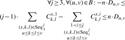(8)

Constraints (7) and (8) describe how k-way junctions are inserted. Constraint (7) restricts the number of inserted motifs with three or more components to one, which is a reasonable assumption given the size of the RNAs. Combined with (8), it means that for every conserved base pair (u,v)∈B, a motif can be inserted if all or none of the components are between u and v. This is equivalent, as we can see in Figure 2c, to saying that we can connect the components which are shown in red without creating a pseudo-knot with the base pairs in the secondary structure.

Motifs completeness:

(9)

(10)

(11)

Constraints (9) , (10) and (11) ensure that the insertions of the components in ω respect their order given in the motif. Constraints (9) and (10) require that if C^x,j_k,l is the j-th component of motif x and it is inserted at positions k,l, then at least one (j−1)-th component of the same motif should be inserted five nucleotides above, and one (j+1)-th component after. The last constraint restricts that, since a motif can be inserted many times, the multiplicity of every component should be equal to the multiplicity of the first component.

Secondary structure constraints:

(12)

(13)

(14)

(15)

We conclude by describing the constraints regulating the secondary structure properties. Constraint (12) use the secondary structure to guide the sites of the components by allowing insertions if and only if one extremity overlaps or is stacked on top of a base pair. Constraint (13) forbids two components from overlapping to each other, and prevents base pairs to occur inside a component. Constraint (14) uses the formulation of (Poolsap et al., 2009) to prevent lonely base pairs (i.e. every position in a base pair must also have an adjacent position in a base pair). Constraint (15) limits the number of canonical base pairs δ of S that can be removed.

3 RESULTS

3.1 Implementation

To solve the IP problem, we use the Gurobi optimizer v.4.5.1 (Houston, 2011) API for Python. We ran our benchmark on a Ubuntu-Server 10.04 on a Dell PE T610 2x Intel Quad core X5570 Xeon Processor, 2.93 GHz 8 M Cache, 64 GB Memory (8×8 GB), 1333 MHz Dual Ranked RDIMMs for 15 Processors, Advanced ECC.

3.2 Dataset

We validate our method on the dataset defined by (Laing and Schlick, 2010) to benchmark the RNA 3D structure prediction programs. In this work, we aim to predict the structure of large RNAs with 3-way and 4-way junctions. Small sequences ( < 50 nucleotides) with simpler structures can be accurately predicted using existing methods such as MC-Pipeline or NAST. Therefore, we removed from the dataset sequences with < 50 nucleotides. We also removed RNAs with secondary structures that include pseudo-knots. Indeed, our approach has been designed to use secondary structures predicted by classical secondary structure predictors such as RNAfold and RNAstructure, thus without pseudo-knots. Moreover, our motif database and IP model have not been designed to insert pseudo-knots. We redirect the reader interested in application of IP techniques to the prediction of pseudo-knots to the recent works of Poolsap et al. (2009) and Sato et al. (2011). Our final dataset includes 11 RNAs with sequences of lengths ranging from 53 to 128 nucleotides. We note that 2 of these 11 had no homologous 3-way junctions in our database. We present here the results on the remaining nine RNAs. Eight of them have a 3-way junction and the other a 4-way junction. Importantly, the motifs extracted from these RNAs by RNA3Dmotifs (Djelloul and Denise, 2008) have been removed from our motif database.

For the negative control test, we used a test set composed of the 24 RNAs from the dataset defined by C.Laing and T.Schlick without pseudo-knot, 3 or 4-way junction. Their sizes range from 16 to 77 nucleotides.

3.3 RNA-MoIP pipe-line

Our RNA tertiary structure prediction pipe-line works in three steps. First, secondary structures are predicted using classical predictors such as RNAfold, RNAstructure or unafold. In this work, we generated the input secondary structures with RNAsubopt (Wuchty et al., 1999). We used the default parameters but discarded structures with lonely pairs (i.e stems of length 1). This procedure generated between 1 and 22 secondary structures for each RNA sequence. Nonetheless, the quality of secondary structure predictions is too low on the riboswitch 3D2G from Arabidopsis thaliana and the tRNA 2DU3 from Archaeoglobus fulgidus to accommodate k-way junction motifs insertion. Therefore, we extended our list of suboptimal structures and generated all secondary structures in the range of 4.5 kcal/mol from the mfe. This operation resulted in a total of 242 (resp. 58) secondary structures. We also note that extending the list of suboptimal structures of other RNAs produces identical results. Typically the secondary structure predictors generate lists of suboptimal structures from which it is difficult to extract the best ones. We will see in Section 3.3.2 that our method is able to identify the best candidates in these ensemble predictions.

We apply RNA-MoIP to insert RNA 3D motifs in these secondary structures as described in Section 2.3. The solution with an optimal score, under our objective function (Section 2.3.3) is scripted manually for MC-Sym with the motifs locked in. Due to various MC-Sym features, it is currently difficult to generate automatically these scripts. Hence, the processing of very large sequence datasets remains challenging. We recall that many 3D structures can have the same motif, which is only determined by the sequence. Here we provide all alternative configurations to MC-Sym. Time is a major limitation of MC-Sym. Using our strategy, we show that preprocessing the sequences with RNA-MoIP results in a dramatic time improvement and at the same time improves the accuracy. We set a time limit of 30 min. Then on every set of predicted structures we apply a minimization of steepest-descent until [(G RMS <5 Kcal/mol/A) or (steps >500)] (Parisien and Major, 2008). It is worth noting that MC-Sym was not able to generate a structure in two cases (3E5C and 2GDI), although RNA-MoIP predicted the 3-way junctions at the correct positions.

3.3.1 Negative control

We verify that RNA-MoIP does not predict wrong insertions (i.e. false positives). We use a negative control dataset composed of the 24 RNAs extracted from the dataset of C.Laing and T.Schlick that contain hairpins and interior loops motifs but without pseudo-knots and k-way junctions. Then, we apply the protocol described as in Section 3.3. Our results indicate that no k-way junction have been inserted in the optimal solution returned by RNA-MoIP.

3.3.2 Secondary structure

The identification of the best secondary structures in a list of suboptimals is one major challenges in RNA secondary structure ensemble prediction. As we can see in Table 1, the average base pair accuracy of the secondary structure prediction is ~63%. But when we look at the base pair accuracy of the secondary structures selected by RNA-MoIP (78%) we observe a major improvement of 15% which means that our approach is able to identify the best secondary structures in a pool of candidates. Interestingly, our program is able to extract candidates with a very low rank. For instance, on 2DU3 RNA-MoIP extracts the 163-th candidate with a base pair accuracy of 91% (versus 43% in average) in a pool of 258 structures. Finally, to accommodate motif insertions RNA-MoIP can remove base pairs. Once removed, the ratio of well-predicted base pairs reaches 84%, thus increases by 6%. This experiment demonstrates that the insertion of motifs can help to identify incorrectly predicted base pairs.

Table 1.

The first column shows the PDB identifier of the RNAs. The two following columns show the ratio of well-predicted base pairs in two structures. The former is the structure in the optimal solution of the RNA and the latter is the same structure after RNA-MoIP was applied and removed some base pairs (we highlight in bold the improved scores). There is an average increase of 6% and only one case where it decreased. The fourth column represents the average of well-predicted base pairs for each RNA over all secondary structures considered by RNA-MoIP. The penultimate column shows the rank of the best secondary structure selected by RNA-MoIP in the ordered list of suboptimal secondary structures generated with RNAsubopt, whereas the last column shows the total number of suboptimal secondary structures in that list.

	Percentage of well-predicted base pairs in the predicted secondary structures			Secondary structure selected by RNA-MoIP
PDB	Optimal solution		Average over all secondary structures	Rank in RNAsubopt list	Nb. of candidate secondary structures
	Before	After
3E5C	100	100	100	1	2
1DK1	88	92	82	1	7
1MMS	47	67	49	2	2
2DU3	79	100	44	52	58
3D2G	91	100	43	163	243
2HOJ	68	68	61	13	20
2GDI	96	94	71	10	22
1LNG	100	100	82	1	7
1MFQ	29	31	31	1	4
Average	78	84	63

3.3.3 Three-dimensional structure

We evaluate the quality of our 3D structure predictions using the RMSD and the RNA Interaction Network Fidelity (Gendron et al., 2001) tool, available with the MC-Pipeline at major.iric.ca/MC-Pipeline/. The latter computes the true positive (TP), false positive (FP) and false negative (FN) tertiary structure interactions between the experimental structures deposited in the PDB (Berman et al., 2000) and our predictions, and returns the positive predictive value (PPV) and sensitivity (STY) defined as:

We report our results in Figure 3. Figure 3b shows that RNA-MoIP coupled with MC-Sym is able to predict most of the tertiary structure interactions.

Fig. 3.

(3a) shows the PPV and STY for all the 3D structures generated by our scripts on MC-Sym against the reference on the PDB (Berman et al., 2000). (3b) Shows in green the distribution of the RMSD of the solutions obtained with MC-Sym when the structures of the motifs were given and in blue when only the secondary structure was provided. N.B.: In the latter, the molecules are identified by their size

We show in green in Figure 3b the RMSDs of the solutions obtained with MC-Sym as described in Section 3.3. We recall that each script for MC-Sym is done manually with the positions inside the predicted motifs directly mapped to the pool of corresponding 3D structures, obtained by RNA3Dmotifs from (Djelloul and Denise, 2008). We also recall that (Laing and Schlick, 2010) report that only the two smallest structures were resolved by MC-Fold∣MC-Sym when only the sequence was given. We thus decided to input into the MC-Fold∣MC-Sym pipeline the sequence with the secondary structure selected by RNA-MoIP. Under this scenario, MC-Sym was allowed to run for 48 h. Those results are shown in blue. As we can see, having the secondary structures allowed to solve five of the seven structures. We note that two of them only produced seven solutions in the first half-hour. The largest one took more then 4 h to produce the first results, and had only two solutions after the 48 h. Nonetheless the information given by the motifs allows to our method to predict significantly more accurate results.

Figure 4 shows that our program outperforms other software and produces 3D structures with a RMSD significantly lower than those observed by Laing and Schlick (2010) for other programs. It also shows that our method scales with the length of the RNA better than other approaches.

Fig. 4.

Comparison of the RMSD obtained by RNA-MoIP, MC-Pipeline, iFoldRNA and FARNA by Laing and Schlick (2010). This figure is derived from the data computed by Laing and Schlick (2010) on which we superposed the results obtained by RNA-MoIP and MC-Sym. The dots are the average RMSD shown in Figure 3b. We also show in dotted line the extrapolated RMSD for MC-Sym and in black the best fit for the average RMSD obtained with our pipeline

We completed this analysis by computing the Matthews correlation coefficient (MCC), defined as: , and the running time of our method. We show in Table 2 an overview of the results obtained on each RNA. We note the fast execution time of RNA-MoIP, even when a large number of secondary structures are used. Also, despite a time limit of 30 min, MC-Sym generates good candidates. Noticeably, our RMSD can be as low as 2.23Å for the tRNA 2DU3 and are considerably smaller than those reported by (Laing and Schlick, 2010) (Fig. 4).

Table 2.

In the first column RNA identifiers are followed by an ‘*’ or a ‘#’ to denote that MC-Sym (reps. NAST) failed to predict them, as reported by Laing and Schlick (2010). The second column contains the length of each RNA. The third column contains the number of secondary structure predicted by RNAfold and used as input for RNA-MoIP. The fourth column is the total time (preprocessing and solve) in seconds taken by RNA-MoIP to find an optimal solution for all the secondary structures. The fifth column contains the number of 3D structures generated by MC-Sym with the script made with RNA-MoIP optimal solution. We then have the maximal, average and SD of the MCC. The following three columns present the minimal, average and SD of the RMSD. Finally, the last column indicate the type of junction found in the native structure.

PDB	NTs	RNA-MoIP		Nb. 3D	MCC			RMSD			Structure
		Sec. structs.	Time (s)		Max	Avg	SD	Min	Avg	SD
3E5C	53	2	0.27	0	–	–	–	–	–	–	3-way (riboswitch)
1DK1	57	7	3.11	106	0.88	0.81	0.03	2.95	4.76	0.99	3-way
1MMS*	58	2	0.31	105	0.68	0.63	0.03	5.66	7.65	0.86	3-way
2DU3*	71	58	139.96	7	0.90	0.82	0.04	2.23	2.91	0.44	4-way (tRNA)
3D2G*#	77	243	1268.63	8	0.84	0.80	0.02	5.34	7.35	1.34	3-way (riboswitch)
2HOJ*#	79	20	27.44	155	0.84	0.80	0.01	3.19	7.29	2.31	3-way (riboswitch)
2GDI*	80	22	47.1	0	–	–	–	–	–	–	3-way (riboswitch)
1LNG*	97	7	110.96	146	0.88	0.84	0.02	2.73	6.30	1.91	3-way (SRP)
1MFQ*	128	4	46.06	14	0.77	0.72	0.03	9.07	14.34	5.01	3-way (SRP)

4 DISCUSSION

In this article we demonstrated that large RNA 3D structures can be automatically predicted using a hierarchical approach. We benefits of the progresses accumulated over the last 30 years in the field of RNA secondary structure prediction and, using an IP framework, expands these methods to incorporate the novel local motifs information available in databases. We show that this approach enables us to predict very quickly accurate 3D structures for large RNA sequences ( > 50 nucleotides). By contrast, previous methods were either too slow or too inaccurate on molecules with similar sizes.

We show that motif insertion enables us to identify the best secondary structures in a pool of suboptimal structures. Nonetheless, the choice of the size of the sample set that need to be generated remains an open problem. As illustrated by the 3D2G and 2DU3 experiments, some RNAs may require significantly more suboptimal than those generated by default by RNAsubopt. A simple strategy to reduce the search space would be to cluster those samples and pick representatives structures.

RNA-MoIP demonstrates that we can already benefit from the information accumulated in RNA local motif databases without deriving a new model. This is important because the paucity of the data currently available in these databases prevents us to develop accurate statistical potentials for predicting tertiary structure interactions in high-order motifs such as the k-way junctions.

Therefore, another important issue with RNA-MoIP is the completeness of the motif database. For instance, we have seen that there is no homologous 3-way junction in our database that can be correctly inserted in 3EGZ (riboswitch in H. sapiens) and 2OIU (synthetic ribozyme). To circumvent this limitation, an interesting approach would be to generate highly probable new motifs from the existing ones using isostericity matrices (Stombaugh et al., 2009).

Some of the IP techniques developed here could be re-written using a dynamic programming approach. However, we argue that the IP approach is more flexible and more suited to this problem. Indeed, in our framework the rules of insertions can be easily modified (i.e. adding, removing or changing an equation) whereas a dynamic programming scheme would required a complete re-implementation. This is particularly useful in this case where some motifs present in our databases have specific insertion constraints. This situation is more likely to happen in the future with the growth of RNA local motif databases. Moreover, we demonstrated in this article that our implementation is fast enough for realistic applications.

Finally, our methods are compatible with state-of-the-art IP programs for pseudo-knot predictions (Poolsap et al., 2009; Sato et al., 2011). In future work, we could envision to merge the two models and include new rules for inserting highly sophisticated 3D motifs with long-range interactions, coaxial stacking or base triplets. Beside its inherent flexibility, the development of IP models for RNA structure prediction finds a justification in recent results showing the inapproximability of the prediction of RNA pseudo-knotted secondary structures with a nearest neighbour model (Sheik et al., 2012).

REFERENCES

- Berman H.M., et al. The protein data bank. Nucleic Acids Res. 2000;28:235–242. doi: 10.1093/nar/28.1.235. [DOI] [PMC free article] [PubMed] [Google Scholar]
- Bindewald E., et al. RNAJunction: a database of RNA junctions and kissing loops for three-dimensional structural analysis and nanodesign. Nucleic Acids Res. 2008;36:D392–D397. doi: 10.1093/nar/gkm842. [DOI] [PMC free article] [PubMed] [Google Scholar]
- Cruz J.A., Westhof E. Sequence-based identification of 3D structural modules in RNA with RMDetect. Nat. Meth. 2011;8:513–521. doi: 10.1038/nmeth.1603. [DOI] [PubMed] [Google Scholar]
- Das R., Baker D. Automated de novo prediction of native-like RNA tertiary structures. Proc. Natl. Acad. Sci. USA. 2007;104:14664–14669. doi: 10.1073/pnas.0703836104. [DOI] [PMC free article] [PubMed] [Google Scholar]
- Djelloul M., Denise A. Automated motif extraction and classification in RNA tertiary structures. RNA. 2008;14:2489–2497. doi: 10.1261/rna.1061108. [DOI] [PMC free article] [PubMed] [Google Scholar]
- Do C.B., et al. CONTRAfold: RNA secondary structure prediction without physics-based models. Bioinformatics. 2006;22:e90–e98. doi: 10.1093/bioinformatics/btl246. [DOI] [PubMed] [Google Scholar]
- Frellsen J., et al. A probabilistic model of RNA conformational space. PLoS Comput. Biol. 2009;5:e1000406. doi: 10.1371/journal.pcbi.1000406. [DOI] [PMC free article] [PubMed] [Google Scholar]
- Gendron P., et al. Quantitative analysis of nucleic acid three-dimensional structures. J. Mol. Biol. 2001;308:919–936. doi: 10.1006/jmbi.2001.4626. [DOI] [PubMed] [Google Scholar]
- Hofacker I.L. Curr. Protoc. Bioinform. 2009. RNA secondary structure analysis using the Vienna RNA package. Chapter 12Unit12.2. [DOI] [PubMed] [Google Scholar]
- Houston Texas. Gurobi Optimization, I. 2011. Gurobi optimizer version 4.5.1. Software Program. [Google Scholar]
- Jonikas M.A., et al. Knowledge-based instantiation of full atomic detail into coarse-grain RNA 3D structural models. Bioinformatics. 2009;25:3259–3266. doi: 10.1093/bioinformatics/btp576. [DOI] [PMC free article] [PubMed] [Google Scholar]
- Jossinet F., et al. Assemble: an interactive graphical tool to analyze and build RNA architectures at the 2D and 3D levels. Bioinformatics. 2010;26:2057–2059. doi: 10.1093/bioinformatics/btq321. [DOI] [PMC free article] [PubMed] [Google Scholar]
- Laing C., Schlick T. Computational approaches to 3D modeling of RNA. J. Phys. Condens. Matter. 2010;22:283101. doi: 10.1088/0953-8984/22/28/283101. [DOI] [PMC free article] [PubMed] [Google Scholar]
- Lamiable A., et al. Automated prediction of three-way junction topological families in RNA secondary structures. Comput. Biol. and Chem. 2012;37:1–5. doi: 10.1016/j.compbiolchem.2011.11.001. [DOI] [PubMed] [Google Scholar]
- Lemieux S., Major F. RNA canonical and non-canonical base pairing types: a recognition method and complete repertoire. Nucleic Acids Res. 2002;30:4250–4263. doi: 10.1093/nar/gkf540. [DOI] [PMC free article] [PubMed] [Google Scholar]
- Markham N.R., Zuker M. UNAFold: software for nucleic acid folding and hybridization. Methods Mol. Biol. 2008;453:3–31. doi: 10.1007/978-1-60327-429-6_1. [DOI] [PubMed] [Google Scholar]
- Martinez H.M., et al. RNA2D3D: a program for generating, viewing, and comparing 3-dimensional models of RNA. J. Biomol. Struct. Dyn. 2008;25:669–683. doi: 10.1080/07391102.2008.10531240. [DOI] [PMC free article] [PubMed] [Google Scholar]
- Parisien M., Major F. The MC-Fold and MC-Sym pipeline infers RNA structure from sequence data. Nature. 2008;452:51–55. doi: 10.1038/nature06684. [DOI] [PubMed] [Google Scholar]
- Poolsap U., et al. Prediction of RNA secondary structure with pseudoknots using integer programming. BMC Bioinformatics. 2009;10(Suppl. 1):S38. doi: 10.1186/1471-2105-10-S1-S38. [DOI] [PMC free article] [PubMed] [Google Scholar]
- Reuter J.S., Mathews D.H. RNAstructure: software for RNA secondary structure prediction and analysis. BMC Bioinformatics. 2010;11:129. doi: 10.1186/1471-2105-11-129. [DOI] [PMC free article] [PubMed] [Google Scholar]
- Sarver M., et al. FR3D: finding local and composite recurrent structural motifs in RNA 3D structures. J. Math. Biol. 2008;56:215–252. doi: 10.1007/s00285-007-0110-x. [DOI] [PMC free article] [PubMed] [Google Scholar]
- Sato K., et al. IPknot: fast and accurate prediction of RNA secondary structures with pseudoknots using integer programming. Bioinformatics. 2011;27:i85–i93. doi: 10.1093/bioinformatics/btr215. [DOI] [PMC free article] [PubMed] [Google Scholar]
- Sharma S., et al. iFoldRNA: three-dimensional RNA structure prediction and folding. Bioinformatics. 2008;24:1951–1952. doi: 10.1093/bioinformatics/btn328. [DOI] [PMC free article] [PubMed] [Google Scholar]
- Sheik S., et al. Proceedings the 23rd Annual Symposium on Combinatorial Pattern Matching (CPM 2012). Helsinki, Finland: 2012. Impact of the energy model on the complexity of RNA folding with pseudoknots; pp. 3–5. July 2012. [Google Scholar]
- Stombaugh J., et al. Frequency and isostericity of RNA base pairs. Nucleic Acids Res. 2009;37:2294–2312. doi: 10.1093/nar/gkp011. [DOI] [PMC free article] [PubMed] [Google Scholar]
- Wang Z., Xu J. A conditional random fields method for RNA sequence-structure relationship modeling and conformation sampling. Bioinformatics. 2011;27:i102–i110. doi: 10.1093/bioinformatics/btr232. [DOI] [PMC free article] [PubMed] [Google Scholar]
- Wuchty S., et al. Complete suboptimal folding of RNA and the stability of secondary structures. Biopolymers. 1999;49:145–165. doi: 10.1002/(SICI)1097-0282(199902)49:2<145::AID-BIP4>3.0.CO;2-G. [DOI] [PubMed] [Google Scholar]
- Zakov S., et al. Rich parameterization improves rna structure prediction. RECOMB. 2011:546–562. doi: 10.1089/cmb.2011.0184. [DOI] [PubMed] [Google Scholar]
- zu Siederdissen,C.H., et al. A folding algorithm for extended RNA secondary structures. Bioinformatics. 2011;27:i129–i136. doi: 10.1093/bioinformatics/btr220. [DOI] [PMC free article] [PubMed] [Google Scholar]