Identifying disease sensitive and quantitative trait-relevant biomarkers from multidimensional heterogeneous imaging genetics data via sparse multimodal multitask learning

Abstract

Motivation: Recent advances in brain imaging and high-throughput genotyping techniques enable new approaches to study the influence of genetic and anatomical variations on brain functions and disorders. Traditional association studies typically perform independent and pairwise analysis among neuroimaging measures, cognitive scores and disease status, and ignore the important underlying interacting relationships between these units.

Results: To overcome this limitation, in this article, we propose a new sparse multimodal multitask learning method to reveal complex relationships from gene to brain to symptom. Our main contributions are three-fold: (i) introducing combined structured sparsity regularizations into multimodal multitask learning to integrate multidimensional heterogeneous imaging genetics data and identify multimodal biomarkers; (ii) utilizing a joint classification and regression learning model to identify disease-sensitive and cognition-relevant biomarkers; (iii) deriving a new efficient optimization algorithm to solve our non-smooth objective function and providing rigorous theoretical analysis on the global optimum convergency. Using the imaging genetics data from the Alzheimer's Disease Neuroimaging Initiative database, the effectiveness of the proposed method is demonstrated by clearly improved performance on predicting both cognitive scores and disease status. The identified multimodal biomarkers could predict not only disease status but also cognitive function to help elucidate the biological pathway from gene to brain structure and function, and to cognition and disease.

Availability: Software is publicly available at: http://ranger.uta.edu/%7eheng/multimodal/

Contact: heng@uta.edu; shenli@iupui.edu

1 INTRODUCTION

Recent advances in acquiring multimodal brain imaging and genome-wide array data provide exciting new opportunities to study the influence of genetic variation on brain structure and function. Research in this emerging field, known as imaging genetics, holds great promise for a system biology of the brain to better understand complex neurobiological systems, from genetic determinants to cellular processes to the complex interplay of brain structure, function, behavior and cognition. Analysis of these multimodal datasets will facilitate early diagnosis, deepen mechanistic understanding and improved treatment of brain disorders.

Machine learning methods have been widely employed to predict Alzheimer's disease (AD) status using imaging genetics measures (Batmanghelich et al., 2009; Fan et al., 2008; Hinrichs et al., 2009b; Shen et al., 2010a). Since AD is a neurodegenerative disorder characterized by progressive impairment of memory and other cognitive functions, regression models have also been investigated to predict clinical scores from structural, such as magnetic resonance imaging (MRI), and/or molecular, such as fluorodeoxyglucose positron emission tomography (FDG-PET), neuroimaging data (Stonnington et al., 2010; Walhovd et al., 2010). For example, Walhovd et al. (2010) performed stepwise regression in a pairwise fashion to relate each of MRI and FDG-PET measures of eight candidate regions to each of four Rey's Auditory Verbal Learning Test (RAVLT) memory scores. This univariate approach, however, did not consider either interrelated structures within imaging data or those within cognitive data. Using relevance vector regression, Stonnington et al. (2010) jointly analyzed the voxel-based morphometry (VBM) features extracted from the entire brain to predict each selected clinical score, while the investigations of different clinical scores are independent from each other.

One goal of imaging genetics is to identify genetic risk factors and/or imaging biomarkers via intermediate quantitative traits (QTs, e.g. cognitive memory scores used in this article) on the chain from gene to brain to symptom. Thus, both disease classification and QT prediction are important machine learning tasks. Prior imaging genetics research typically employs a two-step procedure for identifying risk factors and biomarkers: one first determines disease-relevant QTs, and then detects the biomarkers associated with these QTs. Since a QT could be related to many genetic or imaging markers on different pathways that are not all disease specific (e.g. QT 2 and Gene 3 in Fig. 1), an ideal scenario would be to discover only those markers associated with both QT and disease status for a better understanding of the underlying biological pathway specific to the disease.

Fig. 1.

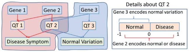
A simplified schematic example of two pathways from gene to QTs to phenotypic endpoints: the red one is disease relevant while the blue one yields only normal variation. Traditional two-stage imaging genetic strategy identifies QT 1 and QT 2 first and then Genes 1, 2, 3. Our new method will identify only disease relevant genes (i.e. Gene 1 and Gene 2); and Gene 3 would not be identified because it cannot be used to classify disease status

On the other hand, identifying genetic and phenotypic biomarkers from large-scale multidimensional heterogeneous data is an important biomedical and biological research topic. Unlike simple feature selection working on a single data source, multimodal learning describes the setting of learning from data where observations are represented by multiple types of feature sets. Many multimodal methods have been developed for classification and clustering purposes, such as co-training (Abney, 2002; Brefeld and Scheffer, 2004; Ghani, 2002; Nigam et al., 2000) and multiview clustering (Bickel and Scheffer, 2004; Dhillon et al., 2003). However, they typically assume that the multimodal feature sets are conditionally independent, which does not hold in many real-world applications such as imaging genetics. Considering different representations give rise to different kernel functions, several Multiple Kernel Learning (MKL) approaches (Bach et al., 2004; Hinrichs et al., 2009a; Kloft et al., 2008; Lanckriet et al., 2004; Rakotomamonjy et al., 2007; Sonnenburg et al., 2006; Suykens et al., 2002; Ye et al., 2008; Yu et al., 2010; Zien and Ong, 2007) have been recently studied and employed to integrate heterogeneous data and select multitype features. However, such models train a single weight for all features from the same modality, i.e. all features from the same data source are weighted equally, when they are combined with the features from other sources. This limitation often yields inadequate performance.

To address the above challenges, we propose a new sparse multimodal multitask learning algorithm that integrates heterogeneous genetic and phenotypic data effectively and efficiently to identify disease-sensitive and cognition-relevant biomarkers from multiple data sources. Different to LASSO (Tibshirani, 1996), group LASSO (Yuan and Lin, 2006) and other related methods that mainly find the biomarkers correlated to each individual QT (memory score), we consider predicting each memory score as a regression task and select biomarkers that tend to play an important role in influencing multiple tasks. A joint classification and regression multitask learning model is utilized to select the biomarkers correlated to memory scores and disease categories simultaneously.

Sparsity regularizations have recently been widely investigated and applied to multitask learning models (Micchelli et al., 2010; Argyriou et al., 2007; Kim and Xing, 2010; Obozinski et al., 2006; Obozinski et al., 2010; Sun et al., 2009). Sparse representations are typically achieved by imposing non-smooth norms as regularizers in the optimization problems. From the view of sparsity organization, we have two types: (i) The flat sparsity is often achieved by ℓ₀-norm or ℓ₁-norm regularizer or trace norm in matrix/tensor completion. Optimization techniques include LARS (Efron et al., 2004), linear gradient search (Liu et al., 2009), proximal methods (Beck and Teboulle, 2009). (ii) The structured sparsity is usually obtained through different sparse regularizers such as ℓ_2,1-norm (Kim and Xing, 2010; Obozinski et al., 2010; Sun et al., 2009), ℓ_2,0-norm (Luo et al., 2010), ℓ_∞,1-norm (Quattoni et al., 2009) (also denoted as ℓ_1,2-norm, ℓ_1,∞-norm in different papers) and group ℓ₁-norm (Yuan and Lin, 2006) which can be solved by methods in Micchelli et al. (2010) and Argyriou et al. (2008). We propose a new combined structured sparse regularization to integrate features from different modalities and to learn a weight for each feature leading to a more flexible scheme for feature selection in data integration, which is illustrated in Figure 3. In our combined structured sparse regularization, the group ℓ₁-norm regularization (blue circles in Fig. 3) learns the feature global importance, i.e. the modal-wise feature importance of every data modality on each class (task), and the ℓ_2,1-norm regularization (red circles in Fig. 3) explores the feature local importance, i.e. the importance of each feature for multiple classes/tasks. The proposed method is applied to identify AD-sensitive biomarkers associated with the cognitive scores by integrating heterogeneous genetic and phenotypic data (as shown in Fig. 2). Our empirical results yield clearly improved performance on predicting both cognitive scores and disease status.

Fig. 3.

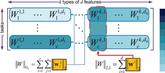
Illustration of the feature weight matrix W^T. The elements in matrix with deep blue color have large values. The group ℓ₁-norm (G₁-norm) emphasizes the learning of the group-wise weights for a type of features (e.g. all the SNPs features, or all the MRI imaging features, or all the FDG-PET imaging features) corresponding to each task (e.g. the prediction for a disease status or a memory score) and the ℓ_2,1-norm accentuates the individual weight learning cross multiple tasks

Fig. 2.

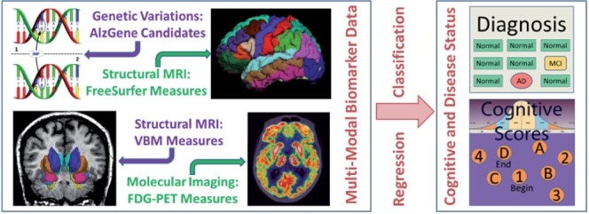
The proposed sparse multimodal multitask feature selection method will identify biomarkers from multimodal heterogeneous data resources. The identified biomarkers could predict not only disease status, but also cognitive functions to help researchers better understand the underlying mechanism from gene to brain structure and function, and to cognition and disease

2 IDENTIFYING DISEASE SENSITIVE AND QT-RELEVANT BIOMARKERS FROM HETEROGENEOUS IMAGING GENETICS DATA

Pairwise univariate correlation analysis can quickly provide important association information between genetic/phenotypic data and QTs. However, it treats the features and the QTs as independent and isolated units, therefore the underlying interacting relationships between the units might be lost. We propose a new sparse multimodal multitask learning model to reveal genetic and phenotypic biomarkers, which are disease sensitive and QT-relevant, by simultaneously and systematically taking into account an ensemble of SNPs (single nucleotide polymorphism) and phenotypic signatures and jointly performing two heterogeneous tasks, i.e. biomarker-to-QT regression and biomarker-to-disease classification. The QTs studied in this article are the cognitive scores.

In multitask learning, given a set of input variables (i.e. features such as SNPs and MRI/PET measures), we are interested in learning a set of related models (e.g. relations between genetic/imaging markers and cognitive scores) to predict multiple outcomes (i.e. tasks such as predicting cognitive scores and disease status). Because these tasks are relevant, they share a common input space. As a result, it is desirable to learn all the models jointly rather than treating each task as independent and fitting each model separately, such as Lasso (Tibshirani, 1996) and group Lasso (Yuan and Lin, 2006). Such multitask learning can discover robust patterns (because significant patterns in a single task could be outliers for other tasks) and potentially increase the predictive power.

In this article, we write matrices as uppercase letters and vectors as boldface lowercase letters. Given a matrix W=[w_ij], its i-th row and j-th column are denoted as wⁱ and w_j, respectively. The ℓ_2,1-norm of the matrix W is defined as ||W||_2,1=∑_i=1||wⁱ||₂ (also denoted as ℓ_1,2-norm by other researchers).

2.1 Heterogeneous data integration via combined structured sparse regularizations

First, we will systematically propose our new multimodal learning method to integrate and select the genetic and phenotypic biomarkers from large-scale heterogeneous data. In the supervised learning setting, we are given n training samples {(x_i, y_i)}ⁿ_i=1, where x_i=(x_i¹,···, x_i^k)^T∈ℜ^d is the input vector including all features from a total of k different modalities and each modality j has d_j features (d=∑_j=1^kd_j). y_i∈ℜ^c is the class label vector of data point x_i (only one element in y_i is 1, and others are zeros), where c is the number of classes (tasks). Let X=[x₁,···, x_n]∈ℜ^d×n and Y=[y₁,···, y_c]∈ℜ^c×n. Different to MKL, we directly learn a d×c parameter matrix as:

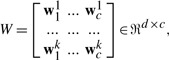(1)

where w_p^q∈ℜ^d_q indicates the weights of all features in the q-th modality with respect to the p-th task (class). Typically, we can use a convex loss function (X, W) to measure the loss incurred by W on the training samples. Compared with MKL approaches that learn one weight for one kernel matrix representing one modality, our method will learn the weight for each feature to capture the local feature importance. Since the features come from heterogeneous data sources, we impose the regularizer (W) to capture the interrelationships of modalities and features as:

(2)

where γ is a trade-off parameter. In heterogeneous data fusion, from multiview perspective of view, the features of a specific view (modality) can be more or less discriminative for different tasks (classes). Thus, we propose a new group ℓ₁-norm (G₁-norm) as a regularization term in Equation (2), which is defined over W as following:

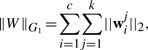(3)

which is illustrated by the blue circles in Figure 3. Then the Equation (2) becomes:

(4)

Since the group ℓ₁-norm uses ℓ₂-norm within each modality and ℓ₁-norm between modalities, it enforces the sparsity between different modalities, i.e. if one modality of features are not discriminative for certain tasks, the objective in Equation (4) will assign zeros (in ideal case, usually they are very small values) to them for corresponding tasks; otherwise, their weights are large. This new group ℓ₁-norm regularizer captures the global relationships between data modalities.

However, in certain cases, even if most features in one modality are not discriminative for the classification or regression tasks, a small number of features in the same modality can still be highly discriminative. From the multitask learning point of view, such important features should be shared by all/most tasks. Thus, we add an additional ℓ_2,1-norm regularizer into Equation (4) as:

(5)

The ℓ_2,1-norm was popularly used in multitask feature selection (Argyriou et al., 2008; Obozinski et al., 2010). Since the ℓ_2,1-norm regularizer impose the sparsity between all features and non-sparsity between tasks, the features that are discriminative for all tasks will get large weights.

Our regularization items consider the heterogeneous features from both group-wise and individual viewpoints. Figure 3 visualizes the matrix W^T as a demonstration. In Figure 3, the elements with deep blue color have large values. The group ℓ₁-norm emphasizes the group-wise weights learning corresponding to each task and the ℓ_2,1-norm accentuates the individual weight learning cross multiple tasks. Through the combined regularizations, for each task (class), many features (not all of them) in the discriminative modalities and a small number of features (may not be none) in the non-discriminative modalities will learn large weights as the important and discriminative features.

The multidimensional data integration has been increasingly important to many biological and biomedical studies. So far, the MKL methods are most widely used. Due to the learning model deficiency, the MKL methods cannot explore both modality-wise importance and individual importance of features simultaneously. Our new structured sparse multimodal learning method integrates the multidimensional data in a more efficient and effective way. The loss function (X, W) in Equation (8) can be replace by either least square loss function or logistic regression loss function to perform regression/classification tasks.

2.2 Joint disease classification and QT regression

Since we are interested in identifying the disease-sensitive and QT-relevant biomarkers, we consider performing both logistic regression for classifying disease status and multivariate regression for predicting cognitive memory scores simultaneously (Wang et al., 2011). A similar model was used in Yang et al. (2009) for heterogeneous multitask learning. Regular multitask learning only considers homogeneous tasks such as regression or classification individually. Joint classification and regression can be regarded as a learning paradigm for handling heterogeneous tasks.

First, logistic regression is used for disease classification, which minimizes the following loss function:

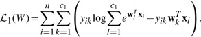(6)

Here, we perform three binary classification tasks for the following three diagnostic groups respectively (c₁=3): AD, mild cognitive impairment (MCI), and health control (HC).

Second, we use the traditional multivariate least squares regression model to predict memory scores. Under the regression matrix P∈ℜ^d×c₂, the least squares loss is defined by

(7)

where X is the data points matrix, P is the coefficient matrix of regression with c₂ tasks, the label matrix .

We perform the joint classification and regression tasks, the disease-sensitive and QT-relevant biomarker identification task can be formulated as the following objective:

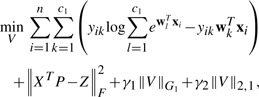(8)

where V=[W P]∈ℜ^{d×(c₁+c₂)}. As a result, the identified biomarkers will be correlated to memory scores and also be discriminative to disease categories.

Since the objective in Equation (8) is a non-smooth problem and cannot be easily solved in general, we derive a new efficient algorithm to solve this problem in the next subsection.

2.3 Optimization algorithm

We take the derivatives of Equation (8) with respect to W and P respectively, and set them to zeros, we have

(9)

(10)

where D_i(1≤i≤c₁+c₂) is a block diagonal matrix with the k-th diagonal block as (I_k is a d_k by d_k identity matrix), D is a diagonal matrix with the k-th diagonal element as . Since D_i(1≤i≤c₁+c₂) and D depend on V = [W P], they are also unknown variables to be optimized. In this article, we provide an iterative algorithm to solve Equation (8). First, we guess a random solution V∈ℜ^{d×(c₁+c₂)}, then we calculate the matrices D_i(1≤i≤c₁+c₂) and D according to the current solution V. After obtaining the D_i(1≤i≤c₁+c₂) and D, we can update the solution V = [W P] based on Equation (9). Specifically, the i-th column of P is updated by pb_i=(XX^T+γ₁D_i+γ₂D)⁻¹Xzb_i. We cannot update W with a closed form solution based on Equation (9), but we can obtained the updated W by the Newton's method. According to Equation (9), we need to solve the following problem:

(11)

Similar to the traditional method in the logistic regression (Krishnapuram et al., 2005; Lee et al., 2006), we can use the Newton's method to obtain the solution W.

For the first term, the traditional logistic regression derivatives can be applied to get the first-and second-order derivatives (Lee et al., 2006).

For the second term, the first-and second-order derivatives are

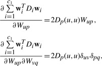(12)

where D_p(u,u) is the u−th diagonal element of D_p.

For the third term, the first-and second-order derivatives are

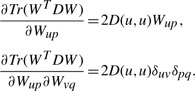(13)

After obtaining the updated solution V=[W P], we can calculate the new matrices D_i(1≤i≤c₁+c₂) and D. This procedure is repeated until the algorithm converges. The detailed algorithm is listed in Algorithm 1. We will prove that the above algorithm will converge to the global optimum.

2.4 Algorithm analysis

To prove the convergence of the proposed algorithm, we need a lemma as follows.

Lemma 1. —

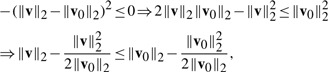
For any vectors v and v₀, we have the following inequality: .

Proof. —

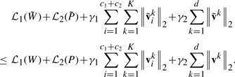
Obviously, −(‖v‖₂−‖v₀‖₂)²≤0, so we have

(14)

which completes the proof. □

Then we prove the convergence of the algorithm, which is described in the following theorem.

Theorem 1. —

The algorithm decreases the objective value of problem (8) in each iteration.

Proof. —

In each iteration, suppose the updated W is , and the updated P is , then the updated V is . From Step 3 in the Algorithm 1, we know that:

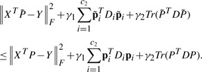
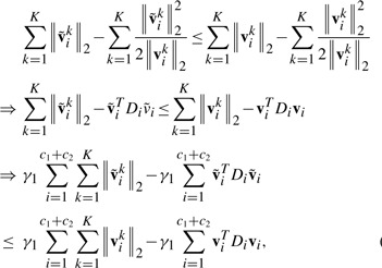
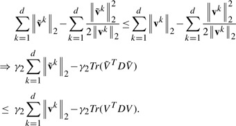
(15)

According to Step 4, we have:

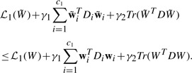
(16)

Based on the definitions of D_i(1≤i≤c₁+c₂) and D, and Lemma 1, we have two following inequalities:

(17)

and

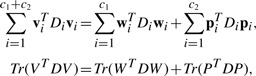
(18)

Note that the following two equalities:

(19)

then by adding Equations (15–18) in the both sides, we arrive at

Therefore, the algorithm decreases the objective value of problem (8) in each iteration. □

In the convergence, W, P, D_i(1≤i≤c₁+c₂) and D satisfy the Equation (9). As the Equation (8) is a convex problem, satisfying the Equation (9) indicates that V=[W P] is a global optimum solution to the Equation (8). Therefore, the Algorithm 1 will converge to the global optimum of the Equation (8). Since our algorithm has the closed form solution in each iteration, the convergency is very fast.

3 EMPIRICAL STUDIES AND DISCUSSIONS

Data used in the preparation of this article were obtained from the Alzheimer's Disease Neuroimaging Initiative (ADNI) database (adni.loni.ucla.edu). One goal of ADNI has been to test whether serial magnetic resonance imaging (MRI), positron emission tomography (PET), other biological markers, and clinical and neuropsychological assessment can be combined to measure the progression of MCI and early AD. For up-to-date information, see www.adni-info.org. Following a prior imaging genetics study (Shen et al., 2010b), 733 non-Hispanic Caucasian participants were included in this study. We empirically evaluate the proposed method by applying it to the ADNI cohort, where a wide range of multimodal biomarkers are examined and selected to predict memory performance measured by five RAVLT scores and classify participants into HC, MCI and AD.

3.1 Experimental design

Overall setting

our primary goal is to identify relevant genetic and imaging biomarkers that can classify disease status and predict memory scores (Fig. 2). We describe our genotyping, imaging and memory data in Section 3.1; present the identified biomarkers in Section 3.2; discuss the disease classification in Section 3.3; and demonstrate the memory score prediction in Section 3.4.

Genotyping data

the single-nucleotide polymorphism data (Saykin et al., 2010) were genotyped using the Human 610-Quad BeadChip (Illumina, Inc., San Diego, CA, USA). Among all SNPs, only SNPs, belonging to the top 40 AD candidate genes listed on the AlzGene database (www.alzgene.org) as of June 10, 2010, were selected after the standard quality control (QC) and imputation steps. The QC criteria for the SNP data include (i) call rate check per subject and per SNP marker, (ii) gender check, (iii) sibling pair identification, (iv) the Hardy–Weinberg equilibrium test, (v) marker removal by the minor allele frequency and (vi) population stratification. The quality-controlled SNPs were then imputed using the MaCH software to estimate the missing genotypes. After that, the Illumina annotation information based on the Genome build 36.2 was used to select a subset of SNPs, belonging or proximal to the top 40 AD candidate genes. This procedure yielded 1224 SNPs, which were annotated with 37 genes (Wang et al., 2012). For the remaining 3 genes, no SNPs were available on the genotyping chip.

Imaging biomarkers

in this study, we use the baseline structural MRI and molecular FDG-PET scans, from which we extract imaging biomarkers. Two widely employed automated MRI analysis techniques were used to process and extract imaging genotypes across the brain from all baseline scans of ADNIA participants as previously described (Shen et al., 2010b). First, VBM (Ashburner and Friston, 2000) was performed to define global gray matter (GM) density maps and extract local GM density values for 86 target regions (Fig. 4a). Second, automated parcellation via freeSurfer V4 (Fischl et al., 2002) was conducted to define 56 volumetric and cortical thickness values (Fig. 4b) and to extract total intracranial volume (ICV). Further information about these measures is available in Shen et al. (2010b). All these measures were adjusted for the baseline age, gender, education, handedness and baseline ICV using the regression weights derived from the healthy control participants. For PET images, following (Landau et al., 2009), mean glucose metabolism (CMglu) measures of 26 regions of interest (ROIs) in the Montreal Neurological Institute (MNI) brain atlas space were employed in this study (Fig. 4c).

Fig. 4.

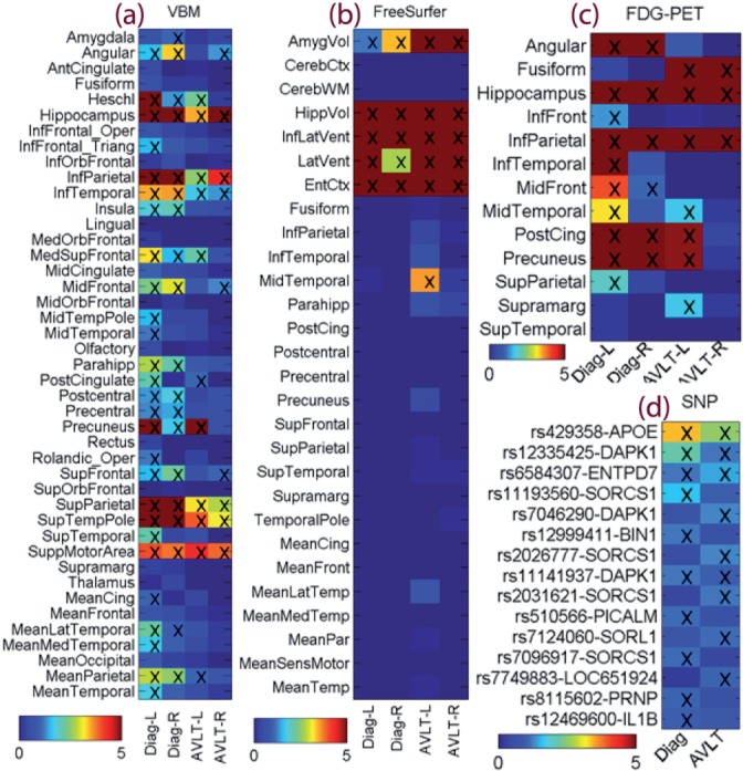
Weight maps for multimodal data: (a) VBM measures from MRI, (b) FreeSurfer measures from MRI, (c) glucose metabolism from FDG-PET, and (d) top SNP findings. Weights for disease classification were labeled as Diag-L (left side), Diag-R (right side) or Diag; and weights for RAVLT regression were labeled as AVLT-L, AVLT-R or AVLT. In (a–c), weights were normalized by dividing the corresponding threshold used for feature selection, and thus all selected features had normalized weights ≥1 and were marked with ‘x’. In (d), only top SNPs were shown, weights were normalized by dividing the weight of the 10th top SNP, and the top 10 SNPs for either classification or regression task had normalized weights ≥1 and were marked with ‘x’

Memory data

The cognitive measures we use to test the proposed method are the baseline RAVLT memory scores from all RADNI participants. The standard RAVLT format starts with a list of 15 unrelated words (List A) repeated over five different trials and participants are asked to repeat. Then the examiner presents a second list of 15 words (List B), and the participant is asked to remember as many words as possible from List A. Trial 6, termed as 5 min recall, requests the participant again to recall as many words as possible from List A, without reading it again. Trial 7, termed as 30 min recall, is administrated in the same way as Trial 6, but after a 30 min delay. Finally, a recognition test with 30 words read aloud, requesting the participant to indicate whether or not each word is on List A. The RAVLT has proven useful in evaluating verbal learning and memory. Table 1 summarizes five RAVLT scores used in our experiments.

Table 1.

RAVLT cognitive measures as responses in multitask learning

Task ID	Description of RAVLT scores
TOTAL	Total score of the first 5 learning trials
TOT6	Trial 6 total number of words recalled
TOTB	List B total number of words recalled
T30	30 minute delay total number of words recalled
RECOG	30 minute delay recognition score

Participant selection

In this study, we included only participants with no missing data for all above four types (views) of features and cognitive scores, which resulted in a set of 345 subjects (83 HC, 174 MCI and 88 AD). The feature sets extracted from baseline multimodal data of these subjects are summarized in Table 2.

Table 2.

Multimodal feature sets as predictors in multiview learning

View ID (feature set ID)	Modality	No. of features
VBM	MRI	86
FreeSurfer	MRI	56
FDG-PET	FDG-PET	26
SNP	Genetics	1244

3.2 Biomarker identifications

The proposed heterogeneous multitask learning scheme aims to identify genetic and phenotypic biomarkers that are associated with both cognition (e.g. RAVLT in this study) and disease status in a joint regression and classification framework. Here we first examine the identified biomarkers. Shown in Figure 4 is a summarization of selected features for all four data types, where the regression/classification weights are color-mapped for each feature and each task.

In Figure 4a, many VBM measures are selected to be associated with disease status, which is in accordance with known global brain atrophy pattern in AD. The VBM measures associated with RAVLT scores seem to be a subset of those disease-sensitive markers, showing a specific memory circuitry contributing to the disease, as well as suggesting that the disease is implicated by not only this memory function but also other complicated factors. Evidently, the proposed method could have a potential to offer deep mechanistic understandings. Shown in Figure 5 is a comparison between RAVLT-relevant markers and AD-relevant markers and their associated weights mapped onto a standard brain space.

Fig. 5.

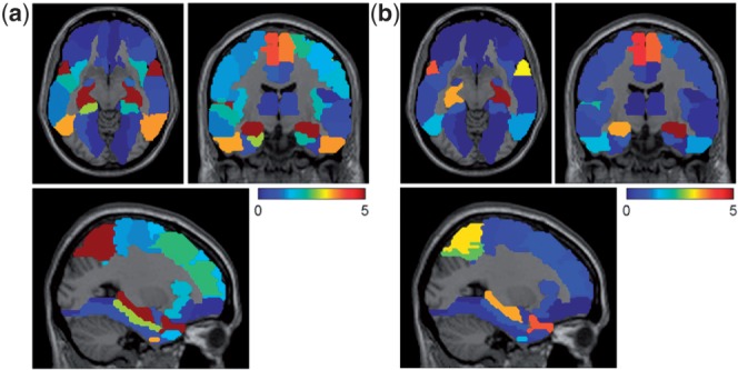
VBM weights of joint regression of AVLT scores and classification of disease status were mapped onto brain (a) Overall weights for disease classification; (b) Overall weights for AVLT regression

Figure 4b shows the identified markers from the FreeSurfer data. In this case, a small set of markers are discovered. These markers, such as hippocampal volume, amygdala volume and entorhinal cortex thickness, are all well-known AD-relevant markers, showing the effectiveness of the proposed method. These markers are also shown to be associated with both AD and RAVLT. The FDG-PET findings (Fig. 4c) are also interesting and promising. The AD-relevant biomarkers include angular, hippocampus, middle temporal and post cingulate regions, which agrees with prior findings e.g. (Landau et al., 2009). Again, a subset of these markers are also relevant to RAVTL scores.

As to the genetics, only top findings are shown in Figure 4d. The APOE E4 SNP (rs429358), the best known AD risk factor, shows the strongest link to both disease status and RAVLT scores. A few other important AD genes, including recently discovered and replicated PICALM and BIN1, are also included in the results. For those newly identified SNPs, further investigation in independent cohorts should be warranted.

3.3 Improved disease classification

We classify the selected participants of ADNI cohort using the proposed methods by integrating the four different types of data. We report the classification performances of our method. We compare our methods against several most recent MKL methods that are able to make use of multiple types of data including SVM ℓ_∞ MKL method (Sonnenburg et al., 2006), SVM ℓ₁ MKL (Lanckriet et al., 2004), SVM ℓ₂ MKL method (Kloft et al., 2008), least square (LSSVM) ℓ_∞ MKL method (Ye et al., 2008), LSSVM ℓ₁ MKL method (Suykens et al., 2002) and LSSVM ℓ₂ MKL method (Yu et al., 2010). We also compare a related method, Heterogeneous Multitask Learning (HML) method (Yang et al., 2009), which simultaneously conducts classification and regression like our method. However, because this method is designed for homogenous input data and is not able to deal with multiple types of data at the same time, we concatenate the four types of features as its input. In addition, we report the classification performances by our method and SVM on each individual types of data as baselines. SVM on a simple concatenation of all four types of features are also reported. In our experiments, we conduct three-class classification, which is more desirable and more challenging than binary classifications using each pair of three categories.

We conduct standard 5-fold cross-validation and report the average results. For each of the five trials, within the training data, an internal 5-fold cross-validation is performed to fine tune the parameters. The parameters of our methods [γ₁ and γ₂ in Equation (8)] are optimized in the range of . For SVM method and MKL methods, one Gaussian kernel is constructed for each type of features , where the parameters γ are fine tuned in the same range used as our method. We implement the MKL methods using the codes published by Yu et al. (2010). Following Yu et al. (2010), in LSSVM ℓ_∞ and ℓ₂ methods, the regularization parameter λ is estimated jointly as the kernel coefficient of an identity matrix; in LSSVM ℓ₁ method, λ is set to 1; in all other SVM approaches, the C parameter of the box constraint is set to 1. We use LIBSVM (http://www.csie.ntu.edu.tw/cjlin/libsvm/) software package to implement SVM. We implement HML method following the details in its original work, and set the parameters to be optimal. The classification performances measured by classification accuracy of all compared methods in AD detection are reported in Table 3.

Table 3.

Classification performance comparison between the proposed method and related methods for distinguishing HC, MCI and AD

Methods	Accuracy (mean + SD)
SVM (SNP)	0.561 ± 0.026
SVM (FreeSurfer)	0.573 ± 0.012
SVM (VBM)	0.541 ± 0.032
SVM (PET)	0.535 ± 0.026
SVM (all)	0.575 ± 0.019
HML (all)	0.638 ± 0.019
SVM ℓ∞ MKL method	0.624 ± 0.031
SVM ℓ1 MKL method	0.593 ± 0.042
SVM ℓ2 MKL method	0.561 ± 0.037
LSSVM ℓ∞ MKL method	0.614 ± 0.031
LSSVM ℓ1 MKL method	0.585 ± 0.018
LSSVM ℓ2 MKL method	0.577 ± 0.033
Our method (SNP)	0.673 ± 0.021
Our method (FreeSurfer)	0.689 ± 0.029
Our method (VBM)	0.669 ± 0.031
Our method (PET)	0.621 ± 0.028
Our method	0.726 ± 0.032

A first glance at the results shows that our methods consistently outperform all other compared methods, which demonstrates the effectiveness of our methods in early AD detection. In addition, the methods using multiple data sources are generally better than their counterparts using one single type of data. This confirms the usefulness of data integration in AD diagnosis. Moreover, our methods always outperform the MKL methods in these experiments, although both take advantage of multiple data sources. This observation is consistent with our theoretical analysis. That is, our methods not only assign proper weight to each type of data, but also consider the relevance of the features inside each individual type of data. In contrast, the MKL methods address the former while not taking into account the latter.

3.4 Improved memory performance prediction

Now we evaluate the memory performance prediction capability of the proposed method. Since the cognitive scores are continuous, we evaluate the proposed method via regression and compare it to two baseline methods, i.e. multivariate linear regression (MRV) and ridge regression. Since both MRV and ridge regression are for single-type input data, we conduct regression on each of the four types of features and a simple concatenation of them. Similarly, we also predict memory performance by our method on the same test conditions. When multiple-type input data are used, as demonstrated in Section 3.2, our method automatically and adaptively select the prominent biomarkers for regression. For each test case, we conduct standard 5-fold cross-validation and report the average results. For each of the five trials, within the training data, an internal 5-fold cross-validation is performed to fine tune the parameters in the range of for both ridge regression and our method. For our method, in each trial, from the learned coefficient matrix we sum the absolute values of the coefficients of a single feature over all the tasks as the overall weight, from which we pick up the features with non-zero weights (i.e. w>10⁻³) to predict regression responses for test data. The performance assessed by root mean square error (RMSE), a widely used measurement for statistical regression analysis, are reported in Table 4.

Table 4.

Comparison of memory prediction performance measured by average RMSEs (smaller is better)

Test case	TOTAL	TOT6	TOTB	T30	RECOG
MRV (SNP)	6.153	2.476	2.168	2.201	3.483
MRV (FreeSurfer)	5.928	2.235	2.039	2.088	3.339
MRV (VBM)	6.093	2.289	2.142	2.137	3.394
MRV (PET)	6.246	2.514	2.237	2.215	3.615
MRV (all)	5.909	2.232	1.992	2.032	3.306
Ridge (SNP)	6.076	2.416	2.147	2.117	3.368
Ridge (FreeSurfer)	5.757	2.203	2.004	2.017	3.237
Ridge (VBM)	5.976	2.147	2.038	2.129	3.249
Ridge (PET)	6.153	2.443	2.186	2.107	3.515
Ridge (all)	5.704	2.143	1.989	1.994	3.193
Our method (SNP)	5.991	2.201	2.008	2.001	3.107
Our method (FreeSurfer)	5.601	2.106	1.947	1.886	3.015
Our method (VBM)	5.715	2.011	1.899	1.974	3.041
Our method (PET)	6.013	2.241	2.017	2.017	3.331
Our method (all)	5.506	1.984	1.886	1.841	2.989

From Table 4 we can see that the proposed method always has better memory prediction performance. Among the test cases, the FreeSurfer imaging measures and VBM imaging measure have similar predictive power, which are better than those of PET imaging measures and SNP features. In general, combining the four types of features are better than only using one type of data. Since our method adaptively weight each type of data and each feature inside a type of data, it has the least regression error when using all available input data. These results, again, demonstrated the usefulness of our method and data integration in early AD diagnosis.

4 CONCLUSIONS

We proposed a novel sparse multimodal multitask learning method to identify the disease-sensitive biomarkers via integrating heterogeneous imaging genetics data. We utilized the joint classification and regression learning model to identify the disease-sensitive and QT-relevant biomarkers. We introduced a novel combined structured sparsity regularization to integrate heterogeneous imaging genetics data, and derived a new efficient optimization algorithm to solve our non-smooth objective function and followed with the rigorous theoretical analysis on the global convergency. The empirical results showed our method improved both memory scores prediction and disease classification accuracy.

REFERENCES

- Abney S. Bootstrapping. Annual Meeting of the Association for Computational Linguistics. 2002:360–367. [Google Scholar]
- Argyriou A., et al. Advances in Neural Information Processing System (NIPS) The MIT Press; 2007. Multi-task feature learning; pp. 41–48. [Google Scholar]
- Argyriou A., et al. Convex multitask feature learning. Machine Learning. 2008;73:243–272. [Google Scholar]
- Ashburner J., Friston K. Voxel-based morphometry–the methods. Neuroimage. 2000;11:805–821. doi: 10.1006/nimg.2000.0582. [DOI] [PubMed] [Google Scholar]
- Bach F., et al. International Conference on Machine Learning (ICML) ACM; 2004. Multiple Kernel Learning, Conic Duality, and the SMOAlgorithm; p. 6. [Google Scholar]
- Batmanghelich N., et al. A general and unifying framework for feature construction, in image-based pattern classification. Inf Process Med Imaging. 2009;21:423–434. doi: 10.1007/978-3-642-02498-6_35. [DOI] [PubMed] [Google Scholar]
- Beck A., Teboulle.,M. A fast iterative shrinkage-thresholding algorithm for linear inverse problems. SIAM J. Imaging Sci. 2009;2:183–202. [Google Scholar]
- Bickel S., Scheffer T. IEEE International Conference on Data Mining (ICDM) 2004. Multi-view clustering; p. 36. [Google Scholar]
- Brefeld U., Scheffer T. International Conference on Machine Learning (ICML) ACM; 2004. Co-em support vector learning; p. 16. [Google Scholar]
- Dhillon I.S., et al. ACM SIGKDD (Special Interest Group on Knowledge Discovery and Data Mining) International Conference on Knowledge Discovery and Data Mining. 2003. Information-theoretic co-clustering; pp. 89–98. [Google Scholar]
- Efron B., et al. Least angle regression. Ann. Stat. 2004;32:407–499. [Google Scholar]
- Fan Y., et al. Spatial patterns of brain atrophy in MCI patients, identified via high-dimensional pattern classification, predict subsequent cognitive decline. Neuroimage. 2008;39:1731–1743. doi: 10.1016/j.neuroimage.2007.10.031. [DOI] [PMC free article] [PubMed] [Google Scholar]
- Fischl B., et al. Whole brain segmentation: automated labeling of neuroanatomical structures in the human brain. Neuron. 2002;33:341–355. doi: 10.1016/s0896-6273(02)00569-x. [DOI] [PubMed] [Google Scholar]
- Ghani R. International Conference on Machine Learning. ACM; 2002. Combining labeled and unlabeled data for multi-class text categorization; pp. 187–194. [Google Scholar]
- Hinrichs C., et al. Proceedings of the 12th International Conference on Medical Image Computing and Computer-Assisted Intervention: Part II. 2009a. MKL for robust multi-modality ad classification; pp. 786–794. [DOI] [PMC free article] [PubMed] [Google Scholar]
- Hinrichs C., et al. Spatially augmented LPboosting for AD classification with evaluations on the ADNI dataset. Neuroimage. 2009b;48:138–149. doi: 10.1016/j.neuroimage.2009.05.056. [DOI] [PMC free article] [PubMed] [Google Scholar]
- Kim S., Xing E. International Conference on Machine Learning (ICML). 2010. Tree-Guided Group Lasso for Multi-Task Regression with Structured Sparsity; pp. 352–359. [Google Scholar]
- Kloft M., et al. Proceedings of the NIPS Workshop on Kernel Learning: Automatic Selection of Optimal Kernels. 2008. Non-sparse multiple kernel learning. [Google Scholar]
- Krishnapuram B., et al. Sparse multinomial logistic regression: fast algorithms and generalization bounds. In. IEEE Trans. Pattern Anal. Mach. Intell. 2005;27:957–968. doi: 10.1109/TPAMI.2005.127. [DOI] [PubMed] [Google Scholar]
- Lanckriet G., et al. Learning the kernel matrix with semidefinite programming. JMLR. 2004;5:27–72. [Google Scholar]
- Landau S., et al. Associations between cognitive, functional, and FDG-PET measures of decline in AD and MCI. Neurobiol. Aging. 2009;32:1207–1218. doi: 10.1016/j.neurobiolaging.2009.07.002. [DOI] [PMC free article] [PubMed] [Google Scholar]
- Lee S.-I., et al. The 21st National Conference on Artificial Intelligence (AAAI) 2006. Efficient l1 regularized logistic regression; p. 401. [Google Scholar]
- Liu J., et al. ACM SIGKDD International Conference on Knowledge Discovery and Data Mining. 2009. Large-scale sparse logistic regression; pp. 547–556. [Google Scholar]
- Luo D., et al. IEEE International Conference on Data Mining (ICDM) 2010. Towards structural sparsity: an explicitl2/l0approach; pp. 344–353. [Google Scholar]
- Micchelli C., et al. Advances in Neural Information Processing System (NIPS) The MIT Press; 2010. A family of penalty functions for structured sparsity; pp. 1612–1623. [Google Scholar]
- Nigam K., et al. Text classification from labeled and unlabeled documents using em. Machine Learning. 2000;39:103–134. [Google Scholar]
- Obozinski G., et al. Multi-task feature selection. Berkeley: Technical report, Department of Statistics, University of California; 2006. [Google Scholar]
- Obozinski G., et al. Joint covariate selection and joint subspace selection for multiple classification problems. Stat. Comput. 2010;20:231–252. [Google Scholar]
- Quattoni A., et al. International Conference on Machine Learning (ICML) ACM; 2009. An efficient projection forl1,∞regularization; pp. 857–864. [Google Scholar]
- Rakotomamonjy A., et al. International Conference on Machine Learning (ICML) ACM; 2007. More efficiency in multiple kernel learning; pp. 775–782. [Google Scholar]
- Saykin A.J., et al. Alzheimer's disease neuroimaging initiative biomarkers as quantitative phenotypes: genetics core aims, progress, and plans. Alzheimers Dement. 2010;6:265–273. doi: 10.1016/j.jalz.2010.03.013. [DOI] [PMC free article] [PubMed] [Google Scholar]
- Shen L., et al. Sparse bayesian learning for identifying imaging biomarkers in AD prediction. Med. Image Comput. Comput. Assist. Interv. 2010a;13(Pt 3):611–618. doi: 10.1007/978-3-642-15711-0_76. [DOI] [PMC free article] [PubMed] [Google Scholar]
- Shen L., et al. Whole genome association study of brain-wide imaging phenotypes for identifying quantitative trait loci in MCI and AD: A study of the ADNI cohort. Neuroimage. 2010b;53:1051–1063. doi: 10.1016/j.neuroimage.2010.01.042. [DOI] [PMC free article] [PubMed] [Google Scholar]
- Sonnenburg S., et al. Large scale multiple kernel learning. In. JMLR. 2006;7:1531–1565. [Google Scholar]
- Stonnington C.M., et al. Predicting clinical scores from magnetic resonance scans in alzheimer's disease. Neuroimage. 2010;51:1405–1413. doi: 10.1016/j.neuroimage.2010.03.051. [DOI] [PMC free article] [PubMed] [Google Scholar]
- Sun L., et al. Advances in Neural Information Processing Systems (NIPS) 22. The MIT Press; 2009. Efficient recovery of jointly sparse vectors; pp. 1812–1820. [Google Scholar]
- Suykens J., et al. Least Squares Support Vector Machines. Singapore: World Scientific; 2002. (ISBN 981-238-151-1) [Google Scholar]
- Tibshirani R. Regression shrinkage and selection via the LASSO. J. R. Statist. Soc B. 1996;58:267–288. [Google Scholar]
- Walhovd K., et al. Multi-modal imaging predicts memory performance in normal aging and cognitive decline. Neurobiol. Aging. 2010;31:1107–1121. doi: 10.1016/j.neurobiolaging.2008.08.013. [DOI] [PMC free article] [PubMed] [Google Scholar]
- Wang H., et al. The Proceedings of The 14th International Conference on Medical Image Computing and Computer Assisted Intervention (MICCAI 2011), Lecture Notes in Computer Science (LNCS) 6893. Springer; 2011. Identifying AD-Sensitive and Cognition-Relevant Imaging Biomarkers via Joint Classification and Regression; pp. 115–123. [DOI] [PMC free article] [PubMed] [Google Scholar]
- Wang H., et al. Identifying quantitative trait loci via group-sparse multitask regression and feature selection: an imaging genetics study of the ADNI cohort. Bioinformatics. 2012;28:229–237. doi: 10.1093/bioinformatics/btr649. [DOI] [PMC free article] [PubMed] [Google Scholar]
- Yang X., et al. Advances in Neural Information Processing System (NIPS) The MIT Press; 2009. Heterogeneous multitask learning with joint sparsity constraints; pp. 2151–2159. [Google Scholar]
- Ye J., et al. Multi-class discriminant kernel learning via convex programming. JMLR. 2008;9:719–758. [Google Scholar]
- Yu S., et al. L 2-norm multiple kernel learning and its application to biomedical data fusion. BMC Bioinformatics. 2010;11:309. doi: 10.1186/1471-2105-11-309. [DOI] [PMC free article] [PubMed] [Google Scholar]
- Yuan M., Lin Y. Model selection and estimation in regression with grouped variables. J. R. Stat. Soc. Ser. B. 2006;68:49C–67. [Google Scholar]
- Zien A., Ong C. International Conference on Machine Learning (ICML) ACM; 2007. Multiclass multiple kernel learning; pp. 1191–1198. [Google Scholar]