Detection of allele-specific methylation through a generalized heterogeneous epigenome model

Abstract

Motivations: High-throughput sequencing has made it possible to sequence DNA methylation of a whole genome at the single-base resolution. A sample, however, may contain a number of distinct methylation patterns. For instance, cells of different types and in different developmental stages may have different methylation patterns. Alleles may be differentially methylated, which may partially explain that the large portions of epigenomes from single cell types are partially methylated, and may have major effects on transcriptional output. Approaches relying on DNA sequence polymorphism to identify individual patterns from a mixture of heterogeneous epigenomes are insufficient as methylcytosines occur at a much higher density than SNPs.

Results: We have developed a mixture model-based approach for resolving distinct epigenomes from a heterogeneous sample. In particular, the model is applied to the detection of allele-specific methylation (ASM). The methods are tested on a synthetic methylome and applied to an Arabidopsis single root cell methylome.

Contact: qpeng@cs.ucsd.edu

1 INTRODUCTION

The advancement of high-throughput sequencing has opened up many important areas of applications, one of which is epigenome sequencing. DNA methylation may repress or activate transcription, and is known to be involved in embryogenesis, genomic imprinting and tumorigenesis in mammals, and transposon silencing in plants (Bestor, 2000; Li et al., 1992; Lippman et al., 2004; Rhee et al., 2002; Zhang et al., 2006; Zilberman et al., 2007). To understand the regulation and dynamics of DNA methylation, the locations of the modified cytosines need to be identified. The first single-base resolution mappings of DNA methylation were produced for the whole Arabidopsis thaliana genome (Cokus et al., 2008; Lister et al., 2008) and for selected subsets of sites in the mouse genome (Meissner et al., 2008) using various bisulfite sequencing technologies. DNA methylation is the modification of DNA base cytosine (methylcytosine). A map of DNA methylation at single-base resolution is referred to as methylome or epigenome.

Cells of different types and in different developmental stages may have different methylation patterns. It has been observed that large portions of the Arabidopsis methylomes are partially methylated (Lister et al., 2008). This may be as a result of the sample containing a number of distinct methylomes. Aberrant methylation is also a general feature of cancer genomes. A better understanding of methylation patterns in cancer genomes may lead to both new diagnostic markers and therapies based on the detection of methylation changes occurring early in tumorigenesis (Laird, 2003). In a tumor tissue particularly of an early stage, however, cancerous cells and normal cells are often mixed together. DNA methylation patterns can also act as markers for tracing stem cell expansion and tumor growth (Kim et al., 2005; Shibata and Tavaré, 2006; Yatabe et al., 2001). Making use of methylation patterns in this way requires determining methylation patterns associated with individual cells or cells from the same clone.

When comparing human fibroblast cell IMR90 and H1 embryonic stem cell (ESC) lines, it is observed that IMR90 has a lower level of methylation than H1 ESC (Lister et al., 2009). Both IMR90 and H1 are of a single cell type. While it is expected that large portions (80%) of the X chromosome are partially methylated as the IMR90 cell line is from a female and the DNA methylation is known to play an important role in X chromosome inactivation (Riggs, 1975), it is unexpectedly observed that around 38% of IMR90 autosomes are identified as partially methylated domains (PMD). What is the nature of partial methylations in a single cell type? Might allelic differences contribute to the partial methylations? Answering these questions requires detecting allele-specific methylation (ASM) patterns.

The methylcytosine is sometimes referred to as the fifth DNA base (Lister and Ecker, 2009). Applying methods for detection of single nucleotide polymorphism (SNP) to methylation, however, may present difficulties. Methylcytosine is much more dynamic than nucleotides and observations generally suggest that methylation of a cytosine site is a statistical event. Unlike SNPs where a nucleotide occurs at a rate of 0, 50 or 100% in a diploid individual (if sequencing errors may be ignored), the methylation level at a particular site may fall anywhere in the range from 0% to 100%. Whether a methylcytosine is allele-specific therefore cannot be determined by the site alone. It needs supporting evidence from the neighboring nucleotides.

If a partially methylated cytosine is in the close vicinity of a SNP such that reads are long enough to cover both sites, then it is straightforward to determine from which allele the reads are originated thus determining the methylation level of the respective alleles. Some studies have shown that ASM is associated with SNPs (Kerkel et al., 2008; Shoemaker et al., 2010). The density of methylation across the whole genome, however, is much higher than that of DNA sequence polymorphism. For instance, while there are close to 3 million SNPs discovered in the human genome ~62 million and 45 million methylcytosines were detected in H1 and IMR90 cells (Lister et al., 2009). It has also been observed that changes in cytosine methylation occur at a frequency much greater than that of the DNA sequence mutations (Ossowski et al., 2010; Schmitz et al., 2011). As a result, SNPs are absent in large portions of the methylomes. We will describe a method in this article that detects ASM without the assistance of SNPs. In addition, even though the functionalities of ASM are not well understood except that they play an important role in imprinting (Hellman and Chess, 2007; Kerkel et al., 2008), it seems that the methylation level of an individual cytosine is less important than the overall levels of methylations within a region, which is also in contrast to the SNPs. We, therefore, focus our effort in detecting regions of ASM.

The remainder of the article is organized as follows. A mixture model is described in Section 2 for modeling the outcome of a methylation sequencing experiment where the sample may contain a mixture of heterogeneous epigenomes. It aims at predicting methylation levels for each cytosine in each individual epigenome. Section 3 lays out the details for detecting regions of ASM based on the mixture model and validates the methods on a synthetic methylome. The methods are then applied to an Arabidopsis root cell methylome and the results are listed in Section 4. Section 5 discusses the results and offers some future directions.

2 A MIXTURE MODEL FOR HETEROGENEOUS EPIGENOMES

In bisulfite sequencing experiments, DNA fragments are treated with sodium bisulfite. The process converts unmethylated cytosines into uracils. The sequence of nucleotides (reads) in the converted fragments are subsequently determined by a sequencer. The reads produced by the sequencer are aligned to a reference genome. Usually only uniquely mapped reads are retained. As a result, what we have is a set of reads that are most similar in sequence to their respective mapped locations in the reference genome, which are presumably the genomic origins of the fragments that produced the reads. In addition, each cytosine on every mapped read is labeled as either methylated or unmethylated.

The methylation level of a particular cytosine is computed as follows: if there are x reads that map to the position, and y out of the x reads have at this position a methylcytosine, then the methylation level is y/x. Note that if the read depth at a cytosine position is below a certain threshold, which is determined by the allowed false positive rate, the methylation is not called, i.e. y=0. (Lister et al., 2008)

If the original sample is composed of a mixture of epigenomes, be it from a set of different cell types, tissues or alleles, the mapped reads will reflect the mixture. Our goal is to infer the original makeup of the mixture from the mapped reads. It should be noted that the attainment of the goal depends on whether the original epigenomes are sufficiently heterogeneous so that we may distinguish them.

As we are only concerned with methylation, we restrict the reads to the genomic positions where the methylation level is greater than zero. The epigenomes and reads may be represented as binary strings, where methylcytosine is set to 1 and the remainder to 0. Let R be a set of binary strings, which we assume are the reads produced by a bisulfite sequencing experiment further restricted to methylation sites. For string r∈R, let x_ri be the letter appearing at position i from r; let [r_a, r_b] be the positions that r spans. Let C={c_j | j=1··· k} be the set of natural frequencies of epigenomes, where c_j is the frequency of the j-th epigenome, and k is the total number of epigenomes. When the model is used to detect the ASM of a diploid organism, k equals to 2. Let M={m_ij | i=1··· n, j=1··· k}, where m_ij is the probability of methylation of epigenome j at position i, and n is the length of the epigenome. The probability of observing string r is

where p_rj is the probability that string r originates from epigenome j, and

(1)

The probability of observing the set R is therefore

or equivalently the log likelihood

The optimization goal is to determine parameters C and M such that the probability of observing the set R is maximum, thus best explaining the reads. We estimate array C and matrix M by maximizing the likelihood l,

which can be solved by using the expectation-maximization (EM) algorithm (Dempster et al., 1977). First, we define a membership matrix

where

As the membership of string r with respect to epigenome j is unknown, it is estimated by its expected value as

(2)

The likelihood can then be rewritten as

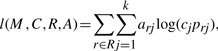(3)

and the optimization becomes

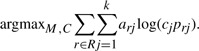Solving the maximization constrained by ∑_j=1^k c_j=1 yields the update equations at each M-step iteration of the EM algorithm as follows (see Appendix A for the detailed derivation),

When the algorithm converges, the matrix M contains the predicted methylation levels for each epigenome in the mixture.

3 DETECTION OF ASM

In this section, we describe how the model is used to detect allele-specific methylated regions in a diploid organism. Notice that ASM is not a precisely defined term. It generally refers to a significant difference between the methylation levels of the two alleles. First, the methylome of a diploid individual is scanned for partially methylated regions (PMRs) as candidates for further analysis. Second, for each candidate region, the reads that align to this region are computationally assigned to the two alleles and the methylation levels of individual cytosines from each allele are estimated. Last, regions are classified to allele-specific or non-specific methylated regions, based on read assignments and the predicted methylation levels from the previous step. A synthetic methylome is used to test the model and to illustrate the details of each step.

We remark that determining whether a read along with its methylcytosines has a higher probability to originate from one allele or the other relies on the differences between the reads, i.e. the methylation states of the cytosines on the reads. The density of methylcytosines of a genome relative to the read length in a sequencing experiment is therefore critical. For instance, if, on average, a read covers at most one methylcytosine, then there is very little hope to deconvolve the allelic methylation states without additional information. While anticipating the rapid growth of the read length in high-throughput sequencing technology, we first tested our method on Arabidopsis thaliana, which has a reasonably high methylation density. The median genomic distance, for instance, between consecutive methylcytosines on Chromosome 1 of A. thaliana Col-0 is 15, while the typical read length of an Illumina sequencer is between 100 and 150 bp presently.

3.1 Identify PMRs as candidates

To detect ASM regions, the whole methylome is scanned for PMRs as candidates, as there is obviously not much difference between the two alleles if the methylation level of a region is near nil or complete. A contiguous methylated region (CMR) refers to a genomic region where the genomic distance between any two consecutive methylcytosines is no larger than a separation threshold s, which is set at around a width comparable to the read length. Each CMR is scanned with a fixed-width sliding window where the window width is the number of methylcytosines. A fixed-width window inside a CMR is classified as a PMR if no fewer than 90% of the methylcytosines are at most 70% methylated (Lister et al., 2009). A PMR may be called with or without a specific lower bound for methylation levels. In the data we have analyzed, the average level of methylations in a CMR is at least 25%, due to that (i) the region has contiguous methylcytosines; (ii) the allowed false positive rate for calling a methylcytosine (Lister et al., 2008) in combination with the sequencing coverage dictates an implicit lower bound on the methylation levels. Consecutive PMRs within the same CMR are merged into a single region.

The dataset being tested is a synthetic methylome that is made up by combining the reads of two methylomes from Arabidopsis root cells: epidermis (Wer+) and endodermis (Scr+). The root cells are obtained by flow sorting; their methylomes by MethylC-Seq bisulfite sequencing (Lister et al., 2008). The genomic length of the reads is 83 bp. The reads from one cell type in the mixture are treated as if they are from one allele of the synthetic methylome. The ASM of the synthetic methylome is, therefore, simulated by cell-specific methylation in the mixture. Forward strand and reverse strand are processed separately.

As ASM and cell-specific methylation arise from different biological processes, the patterns of differential methylations might, therefore, carry signatures unique to each type. The aforementioned synthetic methylome is appropriate for testing cell-specific methylations; yet whether it is a good surrogate for testing ASMs may be questioned. We argue that since the classification is largely based on overall methylation levels within a region rather than relations among methylation levels of individual cytosine sites, the criteria similarly apply to both cell-specific methylation and ASM.

The separation threshold s is set to 100 bp. Each CMR is scanned with a sliding window of width 20, 35 and 50 methylcytosines respectively. Each PMR in the synthetic methylome is labeled as either cell-specific (allele-specific), if no fewer than 90% cytosines in the region are methylated in only one of the two cells, or non-specific otherwise. For the purpose of learning, consecutive windows within the same CMR are merged into one region only if they are labeled as the same type. For a sliding window of width 20, both cell-specific regions and non-specific regions have a median width of 23 methylcytosines. All of the cell-specific regions and around the same number of randomly selected non-specific regions are kept as samples for further analysis. The samples are divided into training and testing samples (Table 1).

Table 1.

Samples of partially methylated regions for classification

	≥20 mC		≥35 mC		≥50 mC
Samples	CS	NS	CS	NS	CS	NS
Training	255	255	42	44	10	10
Testing	100	100	19	21	6	6

mc: methylcytosine; CS: cell-specific; NS: non-specific

3.2 Predict allelic methylation levels

For each PMR, the algorithm described in Section 2 is applied with k=2. For each sample of the synthetic methylome, the reads from the two individual methylomes are mixed together.

One potential problem with the EM algorithm is that it may converge to a local optimum. There are various ways to initialize the parameters. One initialization is to randomly assign each read to a cluster, i.e. set a_rj=1 at probability 1/k. Another option is to set c_j=1/k, and then randomize matrix M. A third option is to randomize the membership matrix A, which appears to be the best option after testing with simulated data. We run the algorithm L times, each with a new random matrix A as the initialization. Let A¹,  A², …, A^L be the membership matrix when each individual run converges, from which two new initializations are derived: A^L+1 and A^L+2, for two additional runs.¹ They are defined as follows: for r∈R, j=1 … k,

Of the total L+2 runs, the one that converges to the largest likelihood is selected. The matrix M yields a predicted level of methylations at each cytosine site. Figure 1 illustrates two samples of PMRs from the synthetic methylome: one cell-specific and the other non-specific. Both experimental and predicted methylation states are shown. The experimental data are from the individual methylomes and are thus treated as golden. The predicted methylation states are used for further classification.

Fig. 1.

Experimental (a and b) versus predicted (c and d) methylation levels of the synthetic methylome. Experimental methylation levels from Wer+ are shown in circles, Scr+ in stars. Two symbols in the bottom figures (c and d) indicate two predicted individual methylomes for the synthetic methylome. The left (a and c) is of an allele-specific region: chromosome 1: [7313026, 7313482] on forward strand. The region contains 50 methylcytosines (mC); 160 reads are aligned to this region. The right (b and d) is of a non-specific region: chromosome 3: [12698733, 12699133] on forward strand. The region contains 42 mC; 367 reads are aligned to the region

3.3 Classify candidate regions with a support vector machine classifier

Once the methylation levels of individual methylcytosines in each allele are estimated and the membership of reads predicted by the model, what remains is to characterize and classify each region based on the estimations. Recall that we used a rather simplistic rule to automatically label the samples in the synthetic methylome when preparing the training and testing samples. The labels are derived from the knowledge of the two individual methylomes making up the synthetic methylome, and therefore are independent of the predictions made by the mixture model. One option is to use the same rule to classify a region from predicted methylation levels. We hope to capture more characteristics of the two classes, however, so multiple measures are employed for this task when it is applied to the real epigenome. We also use the synthetic methylome to train a support vector machine (SVM) classifier that is later used for a real single cell methylome. Notice that the value a_rj gives the probability that the read r is from allele j. If a read needs to be assigned to a single allele, it should be assigned to the j that has the larger value of a_rj, or formally, to cluster j_r=argmax_j (a_rj).

The features for SVM are extracted from the estimated methylation levels (M) and allele frequencies (C). A total of nine features are used (details omitted due to exigencies of space). Both linear and radial basis function (RBF) kernels are tested; the latter yield better performance. Five-fold cross-validation is used to select the best parameters for the kernel function from each training set. The testing results are shown in Table 2. In some of the false positive (FP) samples, both cells have completely unmethylated reads and these reads are clustered together in the synthetic methylome, which are then classified as allele-specific (cell-specific). We hypothesize that these regions have ASM in both individual cell types.

Table 2.

Testing results for classification of partially methylated regions

	≥20 mC		≥35 mC		≥50 mC
Samples	CS	NS	CS	NS	CS	NS
Predicted CS	88 (TP)	13 (FP)	17	3	5	1
Predicted NS	12 (FN)	87 (TN)	2	18	1	5
Accuracy	87.5%		87.5%		83.3%

CS: cell-specific; NS: non-specific

3.4 Identify ASM regions with multiple filters

Using an SVM classifier has its limitations. A classifier trained on one organism will certainly not be appropriate for other organisms. A classifier trained on one cell type may be questionable for another very different type. When parameters for the sequencing experiment change, the classifier should be retrained. In addition, there may not be sufficient data samples for learning at all. Additional measures are therefore necessary for real data.

The Mann–Whitney–Wilcoxon (mww) test is performed on the two clusters resulting from the mixture model. If the null hypothesis is rejected, one cannot readily claim that the methylations are allele-specific. But if on the other hand the null hypothesis is not rejected, it is unlikely that the methylations are allele-specific. Two additional filters are based on methylation rates. One filter is called low methylation rate (lmr). It computes whether one of the two clusters is ≤10% methylated at ≥80% sites. The other is called differential averaged methylation rate (dmr). The averaged methylation rate for each cluster in the region is defined as

and the differential averaged methylation as

We define three classes based on this measure shown in Table 3.

Table 3.

Classes based on differential averaged methylation

d	Class name	Label
[0.0, 0.2]	Similarly methylated	ds
(0.2, 0.9)	Moderately differentially methylated	dm
[0.9, 1.0]	Highly differentially methylated	dh

4 DETECT ASM REGIONS FOR ARABIDOPSIS EPIDERMIS METHYLOME

The methods are applied to the methylome of a single cell type, a root epidermis (Wer+) cell from A. thaliana Col-0. There are a total of 452 partially methylated regions as defined in Section 3.1. The total genomic length of the regions is 84 397 bp, covering 9980 methylcytosines. The 22926 reads are aligned to these regions.

Once the methylation levels of the two alleles and the membership of all reads are predicted by the models, the results are subject to four methods for classification as mentioned in Sections 3.3 and 3.4. Recall that the SVM model is trained on the synthetic methylome made up of two Arabidopsis root methylomes, Wer+ being one of them. Table 4 shows the number of PMRs predicted to be allele-specific by each method and the intersection is taken so as to obtain the most conservative predictions. The first two rows of the table reflect the intersections taken between the d_h class and all other criteria, and d_m class and other criteria, respectively, totaling 34 regions. Table 5 lists the details and annotations for group (1), and Table 6 for group (2). Based on the predicted methylation levels, both groups are highly allele-specific. While one of the two alleles has nearly no methylation, in the first group of 18 regions, the other allele is in general highly methylated; and in the second group of 16 regions, the methylated allele is more partially methylated. An example from each group is shown in Figure 2. If the criteria for ASM are relaxed a bit by removing the rather stringent filter lmr, many more regions [the last row (3) in Table 4] are admitted for further examination. An example from this group is shown in Figure 3.

Table 4.

Predicted ASM regions

Method	svm	lmr	dmr	mww	Intersection
Regions	277	39	dh: 19	362	18(1)
	✓	✓	dm: 368	✓	16(2)
	✓		dm	✓	192(3)

Table 5.

Predicted ASM regions, group (1) in Table 4

ch	Coord start	Coord end	No. of mC	str	Gene model
1	6173395	6173517	20	+	< AT1G17940 −
1	17295458	17295563	24	+	AT1TE57315 −
1	17824930	17825022	20	+	AT1TE59180 −
1	18450185	18450342	20	−	AT1TE61145
1	21929675	21929885	21	+	> AT1G59660
					< AT1G59670
2	7089119	7089281	21	−	AT2G16380 3'UTR +
2	7340522	7340662	23	+	AT2TE29970
					< AT2G16930
2	14386759	14387012	23	+	> AT2G34060
					> AT2G34070 −
3	12092053	12092151	20	+	AT3TE50300 −
3	16726743	16726938	29	−	< AT3G45570
					AT3TE67795 +
4	2367251	2367352	20	+	< AT4G04670
4	10912792	10913005	25	+	> AT4G20210 −
					AT4TE50030 −
4	11932172	11932467	24	+	AT4TE55215 −
					> AT4G22690
					< AT4G22700
4	13269127	13269376	28	−	AT4TE62330
5	5128508	5128716	22	−	AT5TE18530
					> AT5G15725 +
5	8215115	8215303	24	+	AT5TE29690 −
5	22267311	22267477	25	−	AT5TE80145 +
					< AT5G54810
5	26117272	26117538	20	+	AT5TE94040

ch: chromosome; str: strand; < : upstream; > : downstream; Signs in the last column indicate opposite strands.

Table 6.

Predicted ASM regions, group (2) in Table 4

ch	Coord start	Coord end	No. of mC	str	Gene model
1	18054504	18054609	20	−	< AT1G48820 +
					< AT1G48810
1	21249227	21249472	20	+	AT1TE70195 −
					AT1TE70200 −
1	29696108	29696354	26	+	< AT1G78960
2	2168534	2168695	21	−	AT2TE09960
					> AT2G05752
2	11844725	11844944	20	−	AT2TE51520
					> AT2G27780
2	11844762	11845016	25	−	AT2TE51520
					> AT2G27780
3	10865759	10866031	21	+	> AT3TE45185 −
3	12092064	12092269	25	+	AT3TE50300 −
3	16266681	16266822	21	+	AT3TE65915 −
					< AT3G44718 −
3	16934173	16934369	20	−	AT3TE68630 +
					> AT3G46110 +
4	4097347	4097458	20	+	> AT4TE17760
4	4547945	4548048	39	−	AT4TE19110
					< AT4G07747
5	13812896	13813035	21	+	AT5TE49235 −
5	15205421	15205719	23	+	AT5TE55020
5	15268332	15268498	21	−	AT5TE55235
					< AT5G38220 +
5	17406449	17406557	22	+	AT5TE62865 −

ch: chromosome; str: strand; < : upstream; > : downstream; Signs in the last column indicate opposite strands.

Fig. 2.

Read assignments (a and b) and methylation levels (c and d) of the predicted ASM regions of Arabidopsis Wer+ cell. Circle and star symbols in c and d represent two alleles. Lines in top (a and b) figures are restricted reads (solid and dotted lines represent two alleles); small diamonds on lines are methylations. Left (a and c) : a region of Table 4(1): chrom 4: [13269127, 13269376] − strand. Right (b and d) : a region of Table 4(2): chrom 5: [17406449, 17406557] + strand

Fig. 3.

An example from Table 4 group (3): region: chrom 1: [77393, 77508] − strand, 20 mC. (a) reads assignments. (b) predicted methylation levels

Table 7 summarizes the TAIR9 annotations (TAIR, 2009) for all three groups of a total of 226 predicated ASM regions. Many regions overlap with natural transposons as expected; the last row in the table reports the number of regions that have no other annotation than transposon. For the protein coding genes, the gene ontology annotations are summarized in Table 8. One region from group (3), on forward strand of chromosome 1: 11267775 – 11268327, is on the antisense of an exon of protein coding gene AT3G29360, an imprinted gene in A. thaliana seed reported by McKeown et al. (2011). The region has 26 methylcytosines.

Table 7.

Annotation summary of all ASM regions in Table 4

Annotation	Overlap	Upstream	Downstream
Protein coding gene	4 (4) exon	50 (24)	56 (25)
	9 (7) intron
	1 (1) 3′UTR
TE gene	19 (8)	11 (3)	4 (1)
Pseudogene	2	2	3
mi, t, other RNA	1	5 (2)	3
Transposon (only)	66 (39)

Numbers in parenthesis are on the opposite strands. Upstream and downstream are within 1kb.

Table 8.

GO annotation summary for protein coding genes in Table 7

Functional category	Gene body	Upstream	Downstream
Unknown cellular components	2	15	16
Chloroplast	2	8	6
Other intracellular components	2	6	6
Other cellular components		7	6
Other cytoplasmic components	2	6	4
Other membranes	3	4	3
Nucleus	2	2	5
Plastid	1	5	1
Plasma membrane	1	3	3
Unknown molecular functions	2	12	19
Other enzyme activity	5	7	8
Other binding	3	6	6
Protein binding	1	4	3
Transferase activity	2		4
Other molecular functions		4	2
Transferase activity		5
Transporter activity		1	4
Hydrolase activity		3
DNA or RNA binding		3
Nucleotide binding		3
Other metabolic processes	8	19	12
Unknown biological processes	1	17	18
Other cellular processes	4	18	12
Response to stress	4	5	7
Response to abiotic or biotic stimulus		5	6
Transcription,DNA-dependent	1	3	4
Protein metabolism		5	1
Transport		1	4
Others	10	15	10

5 CONCLUSION AND DISCUSSION

We have described a computational model for resolving distinct epigenomes from a heterogeneous sample. In particular, we applied this model to identify allele-specific methylated regions. The reads from potentially multiple epigenomes are mapped to a common reference genome. The goal is essentially to infer the distinct methylation patterns from the mapped reads. Our approach is different from previous attempts in that it does not rely on SNPs, which are few and far between when compared with methylcytosines.

The model was tested on a synthetic methylome. The classification based on the mixture model in conjunction with an SVM classifier yielded an accuracy of 87.5%. Even though the SVM approach is not always applicable to real methylomes, since all the features are derived from the predicted methylation levels and cluster frequencies, the test results reflect the reliability of the predictions made by the model. Additional multiple filters for ASMs may further reduce the number of false positives.

Additional approaches may be employed to validate the methods for ASM detection. One approach is to use ASMs determined with SNP data as ground truth, although such data are presently sparse and anecdotal. Another approach to validate ASM is to use heritable epi-alleles in combination with phasing information obtained from crossing of plants.

We applied the methods to regions of the genome with relatively high density of methylcytosines with each region being treated independently. By taking advantage of pair-end reads and other information, it will also be possible to do phasing and extend and connect the regions. Our model assumes that methylations are independent of each other. Methylations in some regions have a tendency to occur in clusters, which indicates a certain dependency. While our model gives a reasonably good first-order approximation, Markov chain-based models perhaps may be explored to take the dependency into consideration. Identifying ASM is still only at initial research stages. Another direction for future research is to focus on understanding the functionalities of ASM, for instance, how they are related to allele-specific expression.

More complicated heterogeneous epigenome samples may arise from a mixture of various cell types, or a mixture of cancerous cells at various stages, which present yet more and greater challenges than the allelic methylations of a diploid cell. Such samples will enable an ultimate test for the power of the methods. The initial steps are to develop scenarios and criteria for validation as it becomes less obvious what defines cell-specific methylations in the context of multiple cell types.

APPENDIX A

Section 2 described the model for a mixture of epigenomes. This section details the derivation of the update equations at each M-step iteration for the EM algorithm.

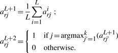
Recall from Section 2 that the optimization goal is to determine the methylation probability matrix M and the epigenome frequency array C such that the likelihood l(M, C, R, A) as defined by Equation (3) is maximized given the set of observed restricted reads R. The membership matrix A is estimated by Equation (2) at each iteration.

As the maximization of likelihood l(M, C, R, A) is constrained by ∑_j=1^k c_j=1, i.e. the epigenome frequencies sum up to 1, we will introduce Lagrange multiplier λ and maximize the unconstrained function

Substituting in p_rj given by Equation (1), we have

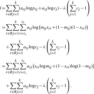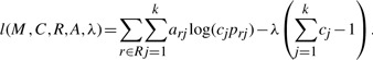
Maximizing l with respect to M, C, λ by setting the respective partial derivatives to zero yields the following set of equations

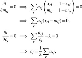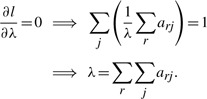Solving for m_ij and substituting in λ for c_j lead to the update equations at each M-step iteration of the EM algorithm as follows,

REFERENCES

- Bestor T.H. The DNA methyltransferases of mammals. Hum. Mol. Genet. 2000;9:2395–2402. doi: 10.1093/hmg/9.16.2395. [DOI] [PubMed] [Google Scholar]
- Cokus S.J., et al. Shotgun bisulphite sequencing of the Arabidopsis genome reveals DNA methylation patterning. Nature. 2008;452:215–219. doi: 10.1038/nature06745. [DOI] [PMC free article] [PubMed] [Google Scholar]
- Dempster A., et al. Maximum likelihood from incomplete data via the EM algorithm. J. R. Stat. Soc. Ser. B. 1977;39:1–38. [Google Scholar]
- Hellman A., Chess A. Gene body-specific methylation on the active X chromosome. Science. 2007;315:1141–1143. doi: 10.1126/science.1136352. [DOI] [PubMed] [Google Scholar]
- Huala E., et al. The Arabidopsis Information Resource (TAIR): a comprehensive database and web-based information retrieval, analysis, and visualization system for a model plant. Nucleic Acids Res. 2001;29:102–105. doi: 10.1093/nar/29.1.102. [DOI] [PMC free article] [PubMed] [Google Scholar]
- Kerkel K., et al. Genomic surveys by methylation-sensitive SNP analysis identify sequence-dependent allele-specific DNA methylation. Nat. Genet. 2008;40:904–908. doi: 10.1038/ng.174. [DOI] [PubMed] [Google Scholar]
- Kim J.Y., et al. Counting human somatic cell replications: Methylation mirrors endometrial stem cell divisions. Proc. Natl. Acad. Sci. USA. 2005;102:17739–17744. doi: 10.1073/pnas.0503976102. [DOI] [PMC free article] [PubMed] [Google Scholar]
- Laird P.W. The power and the promise of DNA methylation markers. Nat. Rev. Cancer. 2003;3:253–266. doi: 10.1038/nrc1045. [DOI] [PubMed] [Google Scholar]
- Li E., et al. Targeted mutation of the DNA methyltransferase gene results in embryonic lethality. Cell. 1992;69:915–926. doi: 10.1016/0092-8674(92)90611-f. [DOI] [PubMed] [Google Scholar]
- Lippman Z., et al. Role of transposable elements in heterochromatin and epigenetic control. Nature. 2004;430:471–476. doi: 10.1038/nature02651. [DOI] [PubMed] [Google Scholar]
- Lister R., Ecker J.R. Finding the fifth base: Genome-wide sequencing of cytosine methylation. Genome Res. 2009;19:959–966. doi: 10.1101/gr.083451.108. [DOI] [PMC free article] [PubMed] [Google Scholar]
- Lister R., et al. Highly integrated single-base resolution maps of the epigenome in Arabidopsis. Cell. 2008;133:523–536. doi: 10.1016/j.cell.2008.03.029. [DOI] [PMC free article] [PubMed] [Google Scholar]
- Lister R., et al. Human DNA methylomes at base resolution show widespread epigenomic differences. Nature. 2009;462:315–322. doi: 10.1038/nature08514. [DOI] [PMC free article] [PubMed] [Google Scholar]
- McKeown P., et al. Identification of imprinted genes subject to parent-of-origin specific expression in arabidopsis thaliana seeds. BMC Plant Biol. 2011;11:113. doi: 10.1186/1471-2229-11-113. [DOI] [PMC free article] [PubMed] [Google Scholar]
- Meissner A., et al. Genome-scale DNA methylation maps of pluripotent and differentiated cells. Nature. 2008;454:766–U91. doi: 10.1038/nature07107. [DOI] [PMC free article] [PubMed] [Google Scholar]
- Ossowski S., et al. The rate and molecular spectrum of spontaneous mutations in Arabidopsis thaliana. Science. 2010;327:92–94. doi: 10.1126/science.1180677. [DOI] [PMC free article] [PubMed] [Google Scholar]
- Rhee I., et al. DNMT1 and DNMT3b cooperate to silence genes in human cancer cells. Nature. 2002;416:552–556. doi: 10.1038/416552a. [DOI] [PubMed] [Google Scholar]
- Riggs A. X inactivation, differentiation, and DNA methylation. Cytogenet. Cell Genet. 1975;14:9–25. doi: 10.1159/000130315. [DOI] [PubMed] [Google Scholar]
- Schmitz R.J., et al. Transgenerational epigenetic instability is a source of novel methylation variants. Science. 2011;334:369–373. doi: 10.1126/science.1212959. [DOI] [PMC free article] [PubMed] [Google Scholar]
- Shibata D., Tavaré S. Counting divisions in a human somatic cell tree: How, what and why? Cell Cycle. 2006;5:610–614. doi: 10.4161/cc.5.6.2570. [DOI] [PubMed] [Google Scholar]
- Shoemaker R., et al. Allele-specific methylation is prevalent and is contributed by CpG-SNPs in the human genome. Genome Res. 2010;20:883–889. doi: 10.1101/gr.104695.109. [DOI] [PMC free article] [PubMed] [Google Scholar]
- Yatabe Y., et al. Investigating stem cells in human colon by using methylation patterns. Proc. Natl. Acad. Sci. USA. 2001;98:10839–10844. doi: 10.1073/pnas.191225998. [DOI] [PMC free article] [PubMed] [Google Scholar]
- Zhang X., et al. Genome-wide high-resolution mapping and functional analysis of DNA methylation in Arabidopsis. Cell. 2006;126:1189–1201. doi: 10.1016/j.cell.2006.08.003. [DOI] [PubMed] [Google Scholar]
- Zilberman D., et al. Genome-wide analysis of Arabidopsis thaliana DNA methylation uncovers an interdependence between methylation and transcription. Nat. Genet. 2007;39:61–69. doi: 10.1038/ng1929. [DOI] [PubMed] [Google Scholar]