Incorporating prior information into association studies

Abstract

Summary: Recent technological developments in measuring genetic variation have ushered in an era of genome-wide association studies which have discovered many genes involved in human disease. Current methods to perform association studies collect genetic information and compare the frequency of variants in individuals with and without the disease. Standard approaches do not take into account any information on whether or not a given variant is likely to have an effect on the disease. We propose a novel method for computing an association statistic which takes into account prior information. Our method improves both power and resolution by 8% and 27%, respectively, over traditional methods for performing association studies when applied to simulations using the HapMap data. Advantages of our method are that it is as simple to apply to association studies as standard methods, the results of the method are interpretable as the method reports p-values, and the method is optimal in its use of prior information in regards to statistical power.

Availability: The method presented herein is available at http://masa.cs.ucla.edu

Contact: eeskin@cs.ucla.edu

1 INTRODUCTION

The cost of collecting genetic information has been decreasing with advances in high-throughput genomic technology (Matsuzaki et al., 2004). Over the last few years, hundreds of genes have been identified as being associated with common human disease (Risch and Merikangas, 1996; Visscher et al., 2012). Traditionally, association studies are performed without making any assumptions about which variants are more or less likely to be involved in the disease. These methods evaluate an association statistic at each single nucleotide polymorphism (SNP), and only take into account one SNP at a time. The Bonferroni correction is often used to control the overall false-positive rate by uniformly limiting the significance threshold at each SNP (Franke et al., 2010).

Current standard approaches report a p-value for each variant and there is a good understanding in the community of what significance levels are required for genome-wide association (Pe'er et al., 2008). Virtually all association studies report p-values as their results which allows investigators to interpret their findings in the context of other groups' findings.

Although the lack of assumptions has the advantage of being unbiased in the search for variants involved in the disease, we know that not all SNPs contribute equally to the disease (Adzhubei et al., 2010). Recent studies (Eskin, 2008) have shown that incorporating prior information such as the results of functional studies (ENCODE Project Consortium, 2007) can increase statistical power. Unfortunately, the methods for incorporating prior information are complicated and difficult to apply in practice. Methods that use prior information are typically Bayesian association study methods (Pe'er et al., 2006; Fridley et al., 2010) and instead report Bayes factors which are not usually reported in other studies. Although standard methods do not take into account prior information, they do have the advantage of being simple.

We present a novel method for performing association studies using prior information, which is as simple to apply as standard association statistics and reports p-values, yet, optimally incorporates prior information. We extend our method to take advantage of the correlation structure to consider multiple markers in a region (de Bakker et al., 2005; Devlin and Risch, 1995). When considering multiple markers, we compute an association statistic at each SNP in the region, not only the collected SNPs. Incorporating prior SNP information increases power over traditional association studies while maintaining the same overall false-positive rate.

Our method can be used in association studies to improve both the power and resolution of a study. When our method is applied to simulations using data from individuals in the HapMap, we demonstrate a significant increase in power and resolution compared with the methods used in a traditional association study. Our method also has the advantage of maintaining the inherent simplicity of a traditional association study. As a result, the computational complexity of our method matches that of a traditional association study.

We measure resolution by calculating the distance between the location of the assumed causal SNP and the location of the SNP corresponding to the maximum-likelihood ratio. Our method increases the average resolution of the four HapMap populations by 27% and the average power by 8% over the traditional method.

Our method has a connection to multithreshold associations presented in (Eskin, 2008). In this work, we show that the multithreshold association method which uses the prior information optimally to maximize statistical power can be interpreted as a likelihood ratio test (LRT). This is the key observation underlying our approach and allows us to propose a very simple method which is also optimal with respect to statistical power, but has the advantage of being simple and easy to interpret.

2 METHODS

2.1 Traditional association studies

Traditional association studies collect m markers in N/2 case and N/2 control individuals. We assume a low-disease prevalence, however, our method can be easily extended to higher prevalence. For each marker i and relative risk γ, the true case allele frequency is defined as follows: p⁺_i=γf_i/((γ−1)f_i+1), where f_i is the population allele frequency. The control allele frequency for the causal maker, p⁻_i, is approximately equal to the population allele frequency, p⁻_i≈f_i. The non-causal markers have equal case and control allele frequencies, that is, p⁺_i = p⁻_i. The overall allele frequency in the case–control sample is, p_i = (p⁺_i+p⁻_i)/2. Let , and be the observed values of the corresponding statistic.

The statistic

(1)

for each marker i is approximately normally distributed with variance 1 and mean non-centrality parameter . The power of a standard association study to detect a significant association at a maker i, relies on the non-centrality parameter and is

where the value of t is the significance threshold, which serves to control the overall false-positive rate, and Φ and Φ⁻¹ denote the cumulative density function (CDF) and the inverse of CDF of the standard normal distribution, respectively. The false-positive rate represents the probability of rejecting the null hypothesis for any marker, assuming there is no causal marker. In our case, we control this probability to α.

If markers are assumed to be independent, the significance threshold is computed using the Bonferroni correction, α_s=α/M. It is important to note that in traditional association studies, the significance threshold, α_s, is fixed for all markers, M.

When computing the overall power of a study, the power is first computed for each marker, . The overall power, defined as 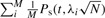, is the average of the power computed at each marker. For clarity, we have assumed that only the markers are the causal variants, which is clearly not realistic; we drop this assumption below.

2.2 Association studies with prior information

Obviously, we do not know which variant is causal and which variant is not causal. However, some variants are more likely involved in the disease than others based on information on how much of a molecular effect that variant has. Let us assume that a marker i has probability c_i of being causal. We define a revised power function that includes prior probabilities

(2)

where α_s is set to control the overall false-positive rate to α.

2.3 Maximizing power in a multithreshold association study

One way to incorporate prior information into association studies is to use multithreshold association (Eskin, 2008). In this approach, we use a different significance threshold at each marker and these thresholds are set to maximize the statistical power taking into account prior information (Adzhubei et al., 2010). We denote the new set of thresholds as variables t₁…t_m. Overall power can be defined as a function of the thresholds t₁…t_m.

(3)

By optimizing the threshold at each marker, we can increase the overall power of a standard association study. Our task is to find the t^*₁…t^*_m that maximizes (3) under the condition that Σt^*_i=α. This constrained optimization can be solved using the method of Lagrange multipliers, assuming the markers are not correlated. Below we show how to use this method to maximize our object function, and as a result find the per marker threshold, t^*₁…t^*_m.

The objective function to maximize is

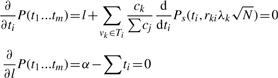
We take the partial derivative of the objective function with respect to t_i and l and set them equal to 0 to obtain

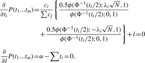(4)

where ϕ is the probability density function (PDF) of the standard normal distribution. See Appendix for the detailed derivation.

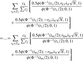
As (4) is true for all marker i∈1…m, we set up the following equality:

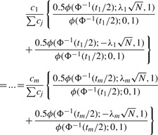(5)

where Σt_i=α. We can numerically find t^*₁…t^*_m satisfying (5). We begin with a guess for c^*, set it equal to (5), and solve for t₁…t_m simultaneously. If Σt_i>α, we decrease c^* (when Σt_i<α, we do otherwise) and repeat the process. The resulting t₁…t_m satisfying the constraint Σt_i=α are denoted t^*₁…t^*_m.

We gain intuition on our method by imagining that we have a total budget of α to distribute among a portfolio of i assets or stocks. Each asset has a certain return on investment, which depends on the t_i, the fraction of the total budget that we allocate to the asset. In order to optimize the total return on our budget of α, we allocate our funds such that the marginal return on investment for each asset is equal. Intuitively, this is because if the marginal return is not equal between investments, we can always increase the overall return by taking out funds from the smaller return investment and put them into the larger return investment. In the case of power, the budget is our overall significance threshold, α. The power return for each marker again depends on the t_i we allocate to each marker. In setting the optimal significance threshold for each marker, we consider the rate of return, or power, which depends on the amount invested, or significance threshold. In determining how to allocate the fraction of the overall significance threshold to each marker, we compute the partial derivative of the power function at each marker and set them equal to each other, which is equivalent to the investment-return analogy.

2.4 Connection to LRT

The key observation in this article is that the multithreshold association has a close connection to the LRT. The LRT compares the likelihood ratio of a statistic with a given threshold C^*, where the likelihood ratio is a direct comparison of the probability of observing the statistic under the null distribution versus the alternative distribution. It is possible to apply the LRT to determine an LRT statistic of a given marker, and thus determine a significance designation for that marker.

Consider the probability of observing the statistic s_i in Equation (1). The null distribution is

and the alternative distribution is, given the non-centrality parameter ,

where the 50:50 mixture is taken assuming that we do not know the direction of the effect (two-sided test). A standard LRT will reject the null hypothesis at s_i if . C^* can be set to control the overall false-positive rate to α.

For the purposes of a multithreshold association study, we will modify the likelihood ratio and the LRT such that the prior information is included,

This likelihood ratio is exactly the same term found in (5). LRT in this case will be done by comparing this likelihood ratio to a number C^*, where

where C^* is the threshold that controls overall false-positive rate to α.

Note that when observed value s_i at marker i is >−Φ⁻¹(t^*_i/2) or <Φ⁻¹(t^*_i/2), then

and we can reject the null hypothesis at i. Thus, LRT and multithreshold association test are equivalent.

When there are correlations between markers, we can still find a C^* such that the chance of  rejecting any of the null hypotheses is α. C^* can be easily calculated using permutation (see Appendix).

2.5 Maximizing power for tag SNPs

Previously, we made the assumption that the markers themselves are causal. Usually, markers are more likely to be tags for the causal variation. Using this information, we can assign each potential polymorphism to the best marker, or tag. We use notation v_k∈T_i to associate each set of polymorphisms v_k to a single marker i. The effect of non-centrality parameter of indirect association is reduced by a factor |r_ki|, where |r_ki| is the correlation coefficient between polymorphism k and marker i (Pritchard and Przeworski, 2001). This correlation coefficient can be determined from reference data such as the (HapMap et al., 2005). We can give each polymorphism a prior probability of being causal c_k. If a polymorphism k is causal, the power function when observing marker i is . Let us denote the total power captured by a marker i as P(t_i,T_i,N). In our case, the total power function of the association study is

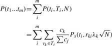This power function can be maximized with respect to t₁…t_m using the same approach as before. There is a constraint that Σt_i=α. The objective function now becomes

We take partial derivatives of this objective function with respect to t_i and α and set them equal to zero

Similarly to Equation (A.3), we can obtain

(6)

In Section 2.4, when markers are assumed to be causal, we detect an association at marker i if the observed statistic s_i at i satisfies

Similarly, when makers themselves are not assumed to be causal, we determine an association at maker i if the statistic s_i at i satisfies

M^* is the threshold that controls false-positive rate to α, the overall significant threshold of the association study. We can determine this M^* by permutation even when there are correlations between markers.

2.6 Multiple-testing adjusted p-value

We can obtain multiple-testing adjusted p-values in our multithreshold association study as follows. In an association study with only one marker, we define the test to be significant if the observed statistic is greater than its threshold Φ⁻¹(α/2). Then, we can use to compute a p-value which measures how significant of an association we observed by using the relationship . For example, in a traditional association study with one marker, if the is ≪0.05, then we can say that this marker strongly associates with the disease. In an association study with m markers, we identify the associated markers by comparing each of the observed statistics against its corresponding cutoff Φ⁻¹(t₁/2),…,Φ⁻¹(t_m/2). To determine how significant the association at each marker is, we need to compute the p-value at that marker. As the cutoff values Φ⁻¹(t₁/2),…,Φ⁻¹(t_m/2) are usually not identical in our multithreshold association study, we compute the multiple-testing adjusted p-values at m markers separately. The multiple-testing adjusted p-value is the probability under the null hypothesis of observing a significant association at any marker.

We compute the adjusted p-value at a marker i by using its observed . If , then the multiple-testing adjusted p-value is α. For , we need to find the p-value . Estimating this significance level is equivalent to finding the and a new set of thresholds t₁^*,…,t_m^* such that when we maximize equation (3) with the constraint , then the cutoff for marker i is . We denote the gradient in Equation (5) at the observed marker i as . As all the partial derivatives of Equation (3) are equal at the optimal solution [Equation (5)], we can determine a new set t₁^*,…,t_m^*, where , by setting each of the gradients in Equation (5) equal to . Finally, the p-value is the sum of t₁^*,…,t_m^*. Once the have been determined, these values are sorted. The marker corresponding to the lowest p-value is the one that is most strongly associated to the disease. Using this approach, we can report a p-value which is adjusted for prior information for each variant.

2.7 New multivariate normal distribution method for correlated markers

In the previous sections, we assumed independent markers 1…m that are possibly correlated to causal variation. However, marker themselves can be correlated to each other. If the markers are correlated, the statistics at the markers follow a multivariate normal distribution (MVN) with variance–covariance matrix Σ, where the entries of Σ are the correlation coefficients between the markers (Han et al., 2009).

Here, we propose a new LRT method designed for the situation that the markers are correlated. By using information from all the markers, we can have better resolution than when inspecting one of the markers.

If variation i is causal and the marker j is correlated to i, the non-centrality parameter at marker j is (Pritchard and Przeworski, 2001). If we consider correlations between variation i and all the markers, the vector of non-centrality parameters with respect to causal variation i will be .

We modify the LRT of the previous section to take into account multiple correlated markers. Given a putative causal variation i, we have the following null hypothesis and the alternate hypothesis at markers 1…m.

Let be the vector of the observed statistics of all markers. The LRT is performed by comparing the probability of under the null and alternative hypothesis, using the formula

(7)

where C^* is set to control the false-positive rate to α and can be found by permutation. ϕ is the PDF of the MVN distribution. Again, the 50:50 mixture of the distributions is taken for the alternative hypothesis to perform two-sided test. When the condition in Equation (7) is satisfied, we have sufficient evidence to reject the null hypothesis at variation i.

It should be noted that the new method is different from the methods we described previously in that the testing is performed per each putative causal variant instead of per each marker. The information of putative causal variants is obtained from the reference dataset, for example, by considering all known variants. This implies increased multiple-testing burden because the number of known variants is much greater than the number of markers in general. However, although the number of tests are considerably increased, the test statistics are highly correlated and therefore the actual multiple-testing burden increases less steeply than the number of tests if we use permutation. Our results show that the new method outperforms previous methods in terms of both power and resolution even after we take into account the increased multiple testing burden.

3 RESULTS

3.1 Candidate gene study associations Project

We follow the evaluation protocol shown in (de Bakker et al., 2005) to simulate association studies in a candidate gene-sized region using the HapMap data ENCODE (ENCODE Project Consortium, 2007). In these simulations, we make case and control individuals by randomly sampling from the pool of haplotypes from HapMap samples in the ENCODE regions. The disease status for each individual is decided by randomly assigning an SNP from this region as causal with a certain relative risk. We assume the scenario where we are using a whole-genome genotyping product such as the Affymetrix 500k SNP chip (Matsuzaki et al., 2004) and where a subset of SNPs from this region are collected as markers. Simulation studies are done over the four HapMap populations in each of the 10 ENCODE regions.

We compare power of four different methods. The first method is the traditional association test where the Bonferroni correction is used. The second method is the multithreshold association test where the markers are assumed to be causal. Since this method only takes into account the non-centrality parameter at each marker, it is equivalent to accounting for the minor allele frequencies (MAFs) of the markers to determine the optimal multithresholds. We call this method multithreshold method with MAF prior. The third method is the multithreshold association test where we assume causal variants are in LD with markers. We use the HapMap data and assign each SNP to a marker by choosing the marker with the highest correlation coefficient with the SNP. This method takes into account not only the non-centrality parameters (or MAF) at the causal variants but also how many causal variants are assigned to each marker and how much the marker and the assigned causal variants are correlated. We call this method multithreshold method with LD and MAF prior. This method is equivalent to the method presented in (Eskin, 2008). The fourth method is the new MVN method where we assume the markers are correlated. The testing is performed at each putative causal variant.

To measure power of each method while correctly accounting for the multiple testing burden of each method, we perform the following simulation procedure. Assuming the null hypothesis of no association, we generate 1000 null panels. We compute the maximum statistic among all markers for all null panels to obtain the empirical null distribution of maximum statistic for each method. The top 5% quantile of the distribution gives us the empirically estimated threshold for α=0.05. Then, we generate 1000 alternative panels assuming the disease model. The power is measured as the number of alternative panels whose maximum statistic exceeds the threshold corresponding to α=0.05. This empirical procedure is shown to accurately control the false-positive rate nearly identical to permuting each panel (de Bakker et al., 2005).

Table 1 shows the power of all four methods. In general, the multithreshold method with MAF prior does not show a better performance than the traditional method. This shows that taking into account only MAF and not the correlations between the marker and the causal variants can be not helpful. The multithreshold method with both LD and MAF prior increases power compared with the traditional method, on average by 1.2%. When we consider only the SNPs whose traditional method's power is in mid-range (between 0.1 and 0.9), the power is increased by a greater amount, 4.0%, which goes along with the results of (Eskin, 2008).

Table 1.

Summary of the power comparison among all 10 ENCODE regions

Pop.	No. of	No. of	All SNPs				SNPs with power between 0.1 and 0.9
	tags	SNPs	Trad	Mult (MAF),	Mult (LD),	MVN,	Trad	Mult (MAF),	Mult (LD),	MVN,
				n (%)	n (%)	n (%)		n (%)	n (%)	n (%)
CEU	678	10 710	0.664	0.660 (−0.6)	0.672 (1.3)	0.697 (5.0)	0.698	0.706 (1.1)	0.733 (5.0)	0.784 (12.2)
YRI	708	13 176	0.445	0.437 (−1.6)	0.451 (1.5)	0.537 (20.8)	0.586	0.577 (−1.6)	0.604 (3.1)	0.731 (24.7)
CHB	606	8934	0.716	0.710 (−0.9)	0.726 (1.4)	0.760 (6.1)	0.708	0.708 (−0.1)	0.740 (4.5)	0.813 (14.7)
JPT	608	9248	0.684	0.675 (−1.4)	0.690 (0.9)	0.722 (5.6)	0.712	0.696 (−2.3)	0.736 (3.4)	0.803 (12.8)
Average			0.627	0.621 (−1.1)	0.635 (1.2)	0.679 (8.3)	0.676	0.671 (−0.7)	0.703 (4.0)	0.782 (15.7)

The numbers in parentheses are the power gain compared with the traditional method

The power increase of the new MVN method is the greatest among all methods. It increases power by 8.3% on average when considering all SNPs and by 15.7% on average when considering the SNPs with mid-range power. The power increase is even as great as 24.7% in the YRI population for the SNPs with mid-range power. This shows that the new MVN method can be very helpful in detecting associations.

We also look at the resolution, by how far the peak association statistic is located from the actual causal variant. We measure this distance in the unit of basepairs and report the results in Table 2. The multithreshold method with MAF prior does not help the resolution either. On the other hand, the multithreshold method with both LD and MAF prior improves the resolution by 2.4% on average for all SNPs and by 4.0% on average for SNPs with mid-range power. However, it failed to improve the resolution in one case (CEU population and for the SNPs with mid-range power).

Table 2.

Summary of the resolution comparison among all 10 ENCODE regions

Pop.	All SNPs				SNPs with power between 0.1 and 0.9
	Trad	Mult (MAF),	Mult (LD),	MVN,	Trad	Mult (MAF),	Mult (LD),	MVN,
		n (%)	n (%)	n (%)		n (%)	n (%)	n (%)
CEU	33 334	33 377 (−0.1)	33 078 (0.8)	27 153 (18.5)	42 983	43 658 (−1.6)	43 040 (−0.1)	27 505 (36.0)
YRI	47 017	49 128 (−4.5)	45 561 (3.1)	30 247 (35.7)	49 245	50 828 (−3.2)	45 690 (7.2)	27 299 (44.6)
CHB	26 582	25 340 (4.7)	25 977 (2.3)	20 045 (24.6)	36 633	35 182 (4.0)	34 875 (4.8)	19 981 (45.5)
JPT	30 740	30 195 (1.8)	29 808 (3.0)	22 917 (25.4)	42 342	40 771 (3.7)	40 731 (3.8)	20 183 (52.3)
Average	34 418	34 510 (−0.3)	33 606 (2.4)	25 090 (27.1)	42 801	42 610 (0.4)	41 084 (4.0)	23 742 (44.5)

The unit of resolution is basepairs. The numbers in parentheses are the improvement percentage in resolution compared with the traditional method

The new MVN method shows the greatest amount of improvement in resolution. The resolution is improved by 27.1% on average for all SNPs and by 44.5% on average for SNPs with mid-range power. This shows that the resolution is so dramatically improved that the distance between the peak association statistic and the causal variant became, on average, almost half compared with the traditional method in the case of the SNPs with mid-range power.

We make an unrealistic assumption that we know the relative risk of the causal polymorphism to be 1.30 and use this assumption to determine the optimal thresholds. We measure the effect of an incorrect assumption by obtaining optimal thresholds at a relative risk of 1.30 and measure the power of these thresholds under a wide range of relative risks. Figure 1 shows the total average power under different relative risks for the traditional method, the multithreshold method with LD and MAF prior, and the new MVN method. Even when the assumed relative risk is incorrect, the multithreshold method and the new MVN method outperform the traditional method.

Fig. 1.

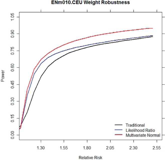
Average power under varying relative risks

3.2 Extrinsic information on candidate gene-sized regions

We measure the impact of extrinsic information on candidate gene-sized regions using the HapMap data ENCODE regions by simulating association studies with unequal priors at the polymorphisms. We first consider the assumption that causal SNPs can be anywhere in the genome, and randomly pick 10% of the variants. Then, we upweight the likelihoods of being causal of these polymorphisms by 25 times. We simulate association studies by picking the causal SNP among these polymorphisms. As we upweight the likelihood of being causal for the actual causal SNP in this simulation, we expect that the methods accounting for the prior information will show a better performance.

In our results, the power increase of the multithreshold method with LD and MAF prior and the MVN method are 2.0% and 11.3% relative to the traditional method, respectively. The amount of power increase is greater compared with when no extrinsic prior information was given (1.2% and 8.3%), as expected. The resolution improvements of the two methods are 5.6% and 55.5%, which are also greater than the improvements we had when no extrinsic prior information was given (4.0% and 15.7%). The most notable change by incorporating extrinsic prior information occurred on the resolution improvement percentage of the MVN method (15.7–55.5%). When considering the SNPs with mid-range power, the resolution improvement of the MVN method relative to the traditional method is as great as 70.4% after incorporating the prior information. This shows that the use of correct prior information can help both the power and the resolution of the methods we proposed, especially the resolution of the MVN method. On the other hand, the power and resolution of the multithreshold method with only MAF prior did not benefit from the extrinsic prior information, possibly because the method only takes into account the markers and not the uncollected putative causal variants.

4 DISCUSSION

We have presented a novel statistical method for incorporating prior information into association studies. The advantage of our method is that we can optimally incorporate prior information with respect to statistical power but still report p-values for each variant. By incorporating the correlation structure underlying the HapMap, we manipulate the significance threshold at each SNP to improve the overall power of a study. Experiments show that our method has a similar computational overhead yet greatly increased power and resolution to traditional association study methods.

Our method has similarities with, the method presented in (Roeder et al., 2007) and (Roeder and Wasserman, 2009). The difference is that while Roeder et al. present the general framework for optimally setting multithresholds for tests, our method is specifically focusing on the context of genetic association studies using available information of both MAF and LD. For example, if only the non-centrality parameter of the statistic at the tested markers is considered as presented in the general framework of Roeder et al., the method will be exactly equivalent to the multithreshold method with MAF prior that we examined in our simulations. We show that this method does not achieve a better performance than the traditional method in terms of both power and resolution. Moreover, we present the novel MVN method that assumes correlation between markers and that outperforms both the traditional method and the multithreshold method of (Eskin, 2008), which is distinctive from the framework assuming independency between the tests.

The new MVN method has some similarities with the weighted haplotype test (Zaitlen et al., 2007) or imputation method (Marchini et al., 2007). In both the new method and their methods, the unobserved causal variant is tested using the observed markers. However, the intrinsic difference is that our method takes into account prior information to optimally set significance thresholds differently to each causal variant in the context of multiple-testing correction. Moreover, the application of the method is much simpler than those methods, requiring only the MAF and LD information from the reference dataset but not the actual haplotype data.

As we use prior information to improve power and resolution, the drawback is that the performance will not be optimal if the prior information is incorrect. For example, the MAF or LD information from the HapMap data can have sampling variation and the extrinsic information about the deleterious effect of the variant can be inaccurate. A possible approach dealing with inaccurate prior information can be explicitly accounting for the uncertainty. For example, we reduce the correlation coefficient estimated from the HapMap by a small amount because the likelihood of the MVN distribution becomes zero if the perfectly correlated markers in the reference is not perfectly correlated in the sample. A systematic approach dealing with prior uncertainty will be an interesting subject of the future research. However, we assume that the uncertainty in the prior information will be decreased in the future as the sample size of the reference dataset increases (1000 Genomes Project Consortium, 2010).

Funding: G.D., D.D., B.H. and E.E. are supported by National Science Foundation grants 0513612, 0731455, 0729049, 0916676 and 1065276, and National Institutes of Health grants K25-HL080079, U01-DA024417, P01-HL30568 and PO1-HL28481. B.H. is supported by the Samsung Scholarship.

Conflict of Interest: None declared.

APPENDIX

A1. Maximizing power in a multithreshold association study

Our task is to find t^*₁…t^*_m that maximize (3) under the condition Σt_i=α. We use the method of Lagrange multipliers to find such t^*₁…t^*_m. This is our objective function

When we take partial derivative with respect to t_i and set it equal to 0, we observe

First, we present the definition of the CDF of the normal distribution:

(A.1)

Now, we present the properties of erf(x).

(A.2)

Now, we consider the power function

where k is the non-centrality parameter.

To maximize the power of a standard association study with respect to t, we find

By applying (A.1), we get

By using (A.2), we get

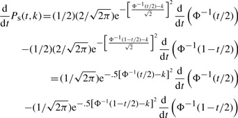(A.3)

Equation (A.3) can be simplified using the property Φ⁻¹ (1−t/2)=−Φ⁻¹(t/2),

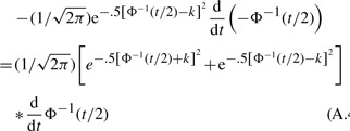(A.4)

Now, we solve for . We use the property:

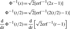(A.5)

and the property:

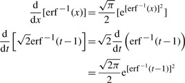(A.6)

Using, (A.5) and (A.6), we find

By plugging this into (A.4), we have

This equation is the likelihood ratio of a random variable s at the value Φ⁻¹(t/2) or equivalently at the value −Φ⁻¹(t/2), between the alternative hypothesis s~0.5N(k,1)+0.5N(−k,1) and the null hypothesis s~N(0,1). The 50:50 mixture of the two symmetrically positioned distributions under the alternative hypothesis can be considered due to the two-sided testing that we perform when we do not have any prior knowledge about the direction of the allele effect.

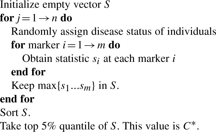
A2. Controlling false-positive rate using permutation

When considering many correlated markers in an association study, we need to find a valid threshold of statistic, C^*, to set the significance threshold for each test such that the overall false-positive rate of the study is controlled to α. The following algorithm is the general method for the permutation procedure, for which the resulting vector allows us to determine a certain C^* to limit the overall false-positive rate of the study. In our example, the 5% quantile of S yields an α level of 0.05.

REFERENCES

- 1000 Genomes Project Consortium. A map of human genome variation from population-scale sequencing. Nature. 2010;467:1061–1073. doi: 10.1038/nature09534. [DOI] [PMC free article] [PubMed] [Google Scholar]
- Adzhubei I.A., et al. A method and server for predicting damaging missense mutations. Nat. Methods. 2010;7:248–249. doi: 10.1038/nmeth0410-248. [DOI] [PMC free article] [PubMed] [Google Scholar]
- Altshuler D., et al. A haplotype map of the human genome. Nature. 2005;437:1299–1320. doi: 10.1038/nature04226. [DOI] [PMC free article] [PubMed] [Google Scholar]
- de Bakker P.I.W., et al. Efficiency and power in genetic association studies. Nat. Genet. 2005;37:1217–1223. doi: 10.1038/ng1669. [DOI] [PubMed] [Google Scholar]
- Devlin B., Risch N. A comparison of linkage disequilibrium measure for fine-scale mapping. Genomics. 1995;29:311–322. doi: 10.1006/geno.1995.9003. [DOI] [PubMed] [Google Scholar]
- ENCODE Project Consortium. Identification and analysis of functional elements in 1% of the human genome by the encode pilot project. Nature. 2007;447:799–816. doi: 10.1038/nature05874. [DOI] [PMC free article] [PubMed] [Google Scholar]
- Eskin E. Increasing power in association studies by using linkage disequilibrium structure and molecular function as prior information. Genome Res. 2008;18:653–660. doi: 10.1101/gr.072785.107. [DOI] [PMC free article] [PubMed] [Google Scholar]
- Franke A., et al. Genome-wide meta-analysis increases to 71 the number of confirmed crohn's disease susceptibility loci. Nat. Genet. 2010;4:1118–1125. doi: 10.1038/ng.717. [DOI] [PMC free article] [PubMed] [Google Scholar]
- Fridley B.L., et al. Bayesian mixture models for the incorporation of prior knowledge to inform genetic association studies. Genet. Epidemiol. 2010;34:418–426. doi: 10.1002/gepi.20494. [DOI] [PMC free article] [PubMed] [Google Scholar]
- Han B., et al. Rapid and accurate multiple testing correction and power estimation for millions of correlated markers. PLoS Genet. 2009;5:1–14. doi: 10.1371/journal.pgen.1000456. [DOI] [PMC free article] [PubMed] [Google Scholar]
- Marchini J., et al. A new multipoint method for genome-wide association studies by imputation of genotypes. Nat. Genet. 2007;39:906–913. doi: 10.1038/ng2088. [DOI] [PubMed] [Google Scholar]
- Matsuzaki H., et al. Genotyping over 100,000 SNPS on a pair of oligonucleotide arrays. Nat. Methods. 2004;1:109–111. doi: 10.1038/nmeth718. [DOI] [PubMed] [Google Scholar]
- Pe'er I., et al. Evaluating and improving power in whole-genome association studies using fixed marker sets. Nat. Genet. 2006;38:663–667. doi: 10.1038/ng1816. [DOI] [PubMed] [Google Scholar]
- Pe'er I., et al. Estimation of the multiple testing burden for genomewide association studies of nearly all common variants. Genet. Epidemiol. 2008;32:381–385. doi: 10.1002/gepi.20303. [DOI] [PubMed] [Google Scholar]
- Pritchard J., Przeworski M. Linkage disequilibrium in humans: models and data. Am. J. Hum. Genet. 2001;69:1–4. doi: 10.1086/321275. [DOI] [PMC free article] [PubMed] [Google Scholar]
- Roeder K., Wasserman L. Genome-wide significance levels and weighted hypothesis testing. Stat. Sci. 2009;24:398–413. doi: 10.1214/09-STS289. [DOI] [PMC free article] [PubMed] [Google Scholar]
- Risch N., Merikangas K. The future of genetic studies of complex human diseases. Science. 1996;273:1516–1517. doi: 10.1126/science.273.5281.1516. [DOI] [PubMed] [Google Scholar]
- Roeder K., et al. Improving power in genome-wide association studies: weights tip the scale. Genet. Epidemiol. 2007;31:741–747. doi: 10.1002/gepi.20237. [DOI] [PubMed] [Google Scholar]
- Visscher P.M., et al. Five years of GWAS discovery. Am. J. Hum. Genet. 2012;90:7–24. doi: 10.1016/j.ajhg.2011.11.029. [DOI] [PMC free article] [PubMed] [Google Scholar]
- Zaitlen N., et al. Leveraging the hapmap correlation structure in association studies. Am. J. Hum. Genet. 2007;80:683–691. doi: 10.1086/513109. [DOI] [PMC free article] [PubMed] [Google Scholar]