Understanding the Phase Contrast Optics to Restore Artifact-free Microscopy Images for Segmentation

Abstract

Phase contrast, a noninvasive microscopy imaging technique, is widely used to capture time-lapse images to monitor the behavior of transparent cells without staining or altering them. Due to the optical principle, phase contrast microscopy images contain artifacts such as the halo and shade-off that hinder image segmentation, a critical step in automated microscopy image analysis. Rather than treating phase contrast microscopy images as general natural images and applying generic image processing techniques on them, we propose to study the optical properties of the phase contrast microscope to model its image formation process. The phase contrast imaging system can be approximated by a linear imaging model. Based on this model and input image properties, we formulate a regularized quadratic cost function to restore artifact-free phase contrast images that directly correspond to the specimen's optical path length. With artifacts removed, high quality segmentation can be achieved by simply thresholding the restored images. The imaging model and restoration method are quantitatively evaluated on microscopy image sequences with thousands of cells captured over several days. We also demonstrate that accurate restoration lays the foundation for high performance in cell detection and tracking.

1. Introduction

Long-term monitoring of living specimens' behavior without staining or altering them has a wide range of applications in biological discovery (Meijering et al., 2009; Rittscher, 2010). Since transparent specimens such as living cells generally lack sufficient contrast to be observed using common light microscopes, the phase contrast imaging technique (Zernike, 1955) was invented to convert the minute light phase variations caused by specimens into changes in light amplitude that can be observed by naked eyes or cameras. Due to the optical principle and some imperfections of the conversion process, phase contrast microscopy images contain artifacts such as the bright halo surrounding the specimen and shade-off (the intensity profile of a large specimen gradually increases from the edges to the center, and even approaches the intensity of the surrounding background medium), as shown in Figure 1(a). Over time, biologists have learned how to overcome or even exploit those artifacts for interpreting phase contrast images. When computer-based microscopy image analysis began to relieve humans from tedious manual labelling (House et al., 2009; Li et al., 2008; Smith et al., 2008; Yang et al., 2005), those artifacts presented significant challenges to automated image processing. In particular, they hinder the process of segmenting images into cells and background, which is the most critical step in almost all cell image analysis applications.

Figure 1.

Cell segmentation and detection by traditional image processing methods. (a) Input phase contrast image; (b) Two-class Otsu thresholding; (c) Three-class Otsu thresholding; (d) Edge detection and morphology tools (from Mathworks product demo: detecting a cell using image segmentation); (e) Marker-controlled watershed; (f) Level-set; (g) LoG filtering (the red crosses denote centroids of detected blobs in the filtered image); (h) LoG filtering with a larger variance σ in the filter.

In the past, many microscopy image segmentation methods have been proposed; for example, thresholding on local intensity value and variation has a long history on cell image segmentation (Otsu, 1979; Wu et al., 1995). The Otsu method calculates the optimal threshold separating the image into two classes such that their intra-class variances are minimal. As shown in Figure 1(b), the halo pixels are classified as one class after Otsu thresholding, and the cell and background pixels are classified as the second class, which is not a satisfactory segmentation result. Realizing the halo artifact in phase contrast images, we can develop a multi-level Otsu thresholding method to segment images into three classes: inner dark cell regions, background and halo. However, as shown in Figure 1(c), the cells are still not well segmented because of the shade-off artifact (intensity similarities between the cell and background classes). House et al. 2009 and Li et al. 2008 explored edge detection and morphology tools to segment cell images. However, if the contrast between cell and background pixels is low, the edge detection and morphological operations might fail the segmentation task as shown in Figure 1(d). Level-set and marker-controlled watershed are two typical gradient-based algorithms used in cell image segmentation (Li et al., 2008; Yang et al., 2005), but these methods are sensitive to local large gradients from the background, as shown in Figures 1(e) and (f). The performance of level-set and marker-controlled watershed also relies on their initializations. Using the halo artifact of phase contrast images, Laplacian-of-Gaussian (LoG) filter is used to detect object blobs (Smith et al., 2008). However, applying a LoG kernel onto a microscopy image containing cells of different sizes, orientations and deformable shapes might not generate satisfactory blob detection results. Different LoG kernels (e.g., different variances in the LoG) may detect different numbers of cells for the same image, as shown in Figures 1(g) and (h). Furthermore, the irregular cell boundaries can not be well located in LoG-filtered images.

The previous microscopy image segmentation methods do not consider the image formation process of microscopy images and treat them in the same manner as natural images. However, there are apparent differences between natural images and phase contrast microscopy images, such as the halo and shade-off. Because of these artifacts, the observed microscopy image intensity does not exactly correspond to the specimen's Optical Path Length (OPL, product of refractive index and thickness). Li and Kanade (2009) proposed an algebraic framework for preconditioning microscopy images captured under Differential Interference Contrast (DIC) microscopes. They use a directional Difference-of-Gaussian kernel to approximate the DIC image formation process and precondition an input DIC image via a linear imaging model. This inspired us to think about whether understanding the phase contrast optics at an early stage will help segment phase contrast images. In fact, we found that those phase contrast artifacts can be well modeled by the optical properties of the image formation process in the phase contrast microscope imaging system. In this paper, we derive a linear imaging model corresponding to the phase contrast optics and formulate a quadratic optimization function to restore the “authentic” phase contrast image without halo or shade-off artifacts. With artifacts removed, high quality segmentation can be achieved by simply thresholding the restored images.

2. Understanding the Phase Contrast Optics

The optical system of a common bright field microscope is shown in Figure 2(a). The light from an illumination source is focused on a specimen plate by a condenser. The light wavefronts illuminate the specimen and divide into two components: one component passes through and around the specimen without deviation (the S wave); and, the other component is diffracted, attenuated and retarded because of the specimen (the D wave). A typical phase retardation caused by living cells in tissue culture is a quarter wave length (Murphy, 2001). The two waves enter the objective lens and combine through interference to produce the particle wave (the P wave) that represents cell pixels in the image. Observing the specimen in a microscopy image depends on the intensity difference between the specimen and its surrounding background, i.e. the amplitude difference between the particle (P) and surround (S) waves. Without any phase contrast technique, the P and S waves have nearly the same wave amplitudes as shown in Figure 2(b), thus the specimen is invisible under a bright field microscope.

Figure 2.

Bright field microscope optics and wave interference. Some of the illuminating waves on the specimen are diffracted, attenuated and retarded (referred to as the D wave). The amplitude difference between the particle (P) and surround (S) waves is too small such that the specimen is transparent and invisible to human eyes.

Compared to the common bright field microscope, phase contrast microscope adds a conjugate pair of condenser annulus and phase plate into its optical system. As shown in Figure 3(a), the specialized annulus is placed at the front focal plane of the condenser and the phase plate is at the rear focal plane of the objective lens (Note: in Figure 3(a), we exaggerate the distance between the phase plate and the virtual intermediate image plane for a clear illustration. In fact, they are very close along the optical axis.) The annulus filters the light from the illumination source such that the specimen is actually illuminated by annular lighting. The phase plate of a positive phase contrast microscope has an etched ring with reduced thickness to advance the surround wave by a quarter wavelength, and it also has a partially absorbing metallic film to attenuate the surround wave. The diffracted wave (D) that is attenuated and retarded by the specimen spreads over the phase plate. Most of the D wave passes through the phase plate without being affected by the phase ring, and it interferes with the surround wave to form the particle wave. As shown in Figure 3(b), with the positive phase contrast technique, the surround wave is advanced and attenuated by the phase ring, and the amplitude difference between the P and S waves is now observable. Furthermore, because the amplitude of the P wave is smaller than that of the S wave, the specimen appears dark on a bright background.

Figure 3.

Phase contrast microscope optics and wave interference. The phase plate separates the surround and diffracted waves, and the surround wave is advanced and attenuated by the phase ring.

Unfortunately, the specimen diffracts the illuminating light to every direction, and a small portion of the diffracted wave leaks into the phase ring (Figure 4(a)). The leaking D wave is advanced and attenuated by the phase ring, and the actual P wave is the interference of three components: S wave, D wave and the leaking D wave. As shown in Figure 4(b), most of the P wave has smaller amplitude than the background S wave so the specimen looks dark. However, a small part of the P wave has larger amplitude than the S wave, which causes the bright halo and shade-off artifacts.

Figure 4.

A small portion of diffracted light leaking into the phase ring causes the halo and shade-off artifacts.

3. Deriving the Phase Contrast Microscopy Imaging Model

Following the optical principle of the phase contrast microscope, we derive its computational imaging model in this section. We assume the illuminating waves arrive at the specimen plate with the same amplitude and phase, and denote them as

$$l\left(\mathbf{x}\right)=A{e}^{i\beta }$$ (1)

where $\mathbf{x}=\{({\mathbf{x}}_j^r,{\mathbf{x}}_j^c),j=1,\cdots ,J\}$ denote 2D locations (row and column) of total J image pixels on the specimen plate, i² = −1, A and β are the illuminating wave's amplitude and phase before hitting the specimen plate.

After illuminating waves pass through the specimen plate, they divide into two components: the unaltered surround wave l_S(x) and the diffracted wave l_D(x) that is attenuated and retarded by the specimen

$$l_S\left(\mathbf{x}\right)=l\left(\mathbf{x}\right)=A{e}^{i\beta }$$ (2)

$$l_D\left(\mathbf{x}\right)={\zeta }_c{e}^{-if\left(\mathbf{x}\right)}l\left(\mathbf{x}\right)={\zeta }_{c}A{e}^{i(\beta -f\left(\mathbf{x}\right))}$$ (3)

where ζ_c is the amplitude attenuation factor and f(x) represents phase shift caused by the specimen at location x. Our goal is to restore f(x), the “authentic” phase contrast image corresponding to the specimen's optical path length without artifacts.

A thin lens with a large aperture essentially performs a spatial Fourier transform ($\mathcal{F}$) on the waves from its front focal plane to its rear focal plane (Gaskill, 1978). Thus, after the surround and diffracted waves pass the objective lens, the waves in front of the phase plate are

$$L_S\left(\mathbf{w}\right)=\mathcal{F}\left(l_S\left(\mathbf{x}\right)\right)$$ (4)

$$L_D\left(\mathbf{w}\right)=\mathcal{F}\left(l_D\left(\mathbf{x}\right)\right).$$ (5)

The phase plate functions as a band-pass filter. For the non-diffracted surround wave, the positive phase ring attenuates the wave amplitude and advances its phase by a quarter wave length (π/2), thus the corresponding transmittance function for the surround wave is

$$T_S\left(\mathbf{w}\right)={\zeta }_p{e}^{i\frac{\pi }{2}}=i{\zeta }_p$$ (6)

where ζ_p represents the amplitude attenuation by a phase ring with outer radius R and width W (Figure 3(a), R and W are provided by microscope manufacturers). The diffracted wave spreads over the phase plate with a small portion leaking into the ring. Its corresponding transmittance function is a band-pass filter

$$T_D\left(\mathbf{w}\right)=\{\begin{array}{cc}i{\zeta }_p\hfill & \text{if}R-W\le w_r\le R\hfill \\ 1\hfill & \text{otherwise}\hfill \end{array}\phantom{\}}$$ (7)

which can be re-written as

$$T_D\left(\mathbf{w}\right)=1+(i{\zeta }_p-1)[\text{cyl}\left(\frac{w_r}{R}\right)-\text{cyl}\left(\frac{w_r}{R-W}\right)]$$ (8)

where $w_r=\sqrt{w_u^2+w_v^2}$ is the radial frequency and cyl(·) is a 2D cylinder function

$$\text{cyl}\left(w\right)=\{\begin{array}{cc}1\hfill & \text{if}0\le w\le 1\hfill \\ 0\hfill & \text{otherwise}.\hfill \end{array}\phantom{\}}$$ (9)

After the band-pass filtering, we have the waves after the phase plate as

$${\tilde{L}}_S\left(\mathbf{w}\right)=L_S\left(\mathbf{w}\right)T_S\left(\mathbf{w}\right)$$ (10)

$${\tilde{L}}_D\left(\mathbf{w}\right)=L_D\left(\mathbf{w}\right)T_D\left(\mathbf{w}\right).$$ (11)

The ocular lens perform another Fourier transform. Mathematically, the forward and inverse Fourier transforms are identical except for a minus sign, and thus, applying Fourier transform on ${\tilde{L}}_S\left(\mathbf{w}\right)$ and ${\tilde{L}}_D\left(\mathbf{w}\right)$ is equivalent to applying inverse Fourier transform on them with a minus sign on the input variable of the resultant function. The waves after the ocular lens are

$${\tilde{l}}_S\left(\mathbf{x}\right)=l_S\left(\mathbf{x}\right)\ast t_S\left(\mathbf{x}\right)$$ (12)

$${\tilde{l}}_D\left(\mathbf{x}\right)=l_D\left(\mathbf{x}\right)\ast t_D\left(\mathbf{x}\right)$$ (13)

where * denotes the convolution operator. t_S(·) and t_D(·) denote the inverse Fourier transform of T_S(·) and T_D(·), respectively. The inverse Fourier transform of T_S(·) (Eq. 6) is

$$t_S\left(\mathbf{x}\right)=i{\zeta }_p\delta \left(\mathbf{x}\right)$$ (14)

where δ(·) is a Dirac delta function. The inverse Fourier transform of T_D(·) (Eq. 8) is (Appendix I)

$$t_D\left(\mathbf{x}\right)=\delta \left(\mathbf{r}\right)+(i{\zeta }_p-1)\text{airy}\left(\mathbf{r}\right)$$ (15)

where airy(r) is an obscured Airy pattern (Born and Wolf, 1997) as shown in Figure 5 where a bright region in the center is surrounded by a series of concentric alternating bright/dark rings.

Figure 5.

An obscured Airy pattern. (a) 3D surface view; (b) 2D view.

Substituting l_S, t_S, l_D, t_D into ${\tilde{l}}_S$ and ${\tilde{l}}_D$ in Eqs. 12 and 13, we get

$${\tilde{l}}_S\left(\mathbf{x}\right)=i{\zeta }_{p}A{e}^{i\beta }$$ (16)

$${\tilde{l}}_D\left(\mathbf{x}\right)={\zeta }_{c}A{e}^{i(\beta -f\left(\mathbf{x}\right))}+(i{\zeta }_p-1){\zeta }_{c}A{e}^{i(\beta -f\left(\mathbf{x}\right))}\ast \text{airy}\left(\mathbf{r}\right)$$ (17)

The first term in Eq. 17 is the primary component of the diffracted wave that destructively interferes with the non-diffracted surround wave and generates the contrast for human observation. The second term in Eq. 17 comes from the diffracted wave leaking into the phase ring which causes the halo and shade-off artifacts. The intensity of the final observed image is computed as (Appendix II)

$$g\left(\mathbf{x}\right)\propto (\delta \left(\mathbf{r}\right)-\text{airy}\left(\mathbf{r}\right))\ast f\left(\mathbf{x}\right)+C$$ (18)

where C is a constant. The convolution kernel in Eq. 18 represents the point spread function (PSF) of the phase contrast microscope

$$\text{PSF}(u,v)=\delta (u,v)-\text{airy}\left(\sqrt{u^2+v^2}\right)$$ (19)

which is a linear operator. Note, in the positive phase contrast microscope, cells appear darker than the surrounding medium. However, in negative phase contrast microscope (surround wave is retarded instead of being advanced), cells appear brighter than the surrounding medium. The corresponding PSF for the negative phase contrast is

$$\text{PSF}(u,v)=\text{airy}\left(\sqrt{u^2+v^2}\right)-\delta (u,v)$$ (20)

In our restoration framework, we use Eq. 20 for both positive and negative phase contrast microscopes such that in restored images, cells are bright while background is dark.

Now we can define the linear imaging model between g (vectorized observed image) and f (vectorized artifact-free phase contrast image to be restored) as

$$\mathbf{g}\approx \mathbf{Hf}+C$$ (21)

In practice, we discretize the PSF kernel as a (2M+1) × (2M+1) matrix (e.g. M = 5) and the H matrix is defined by

$${\left(Hf\right)}_j=\sum _{u=1}^{2M+1}\sum _{v=1}^{2M+1}\text{PSF}(u,v)\mathbf{f}({\mathbf{x}}_j^r+u-M,{\mathbf{x}}_j^c+v-M)$$ (22)

where $\mathbf{x}=\{({\mathbf{x}}_j^r,{\mathbf{x}}_j^c),j=1,\cdots ,J\}$ denote 2D locations (row and column) of total J image pixels on the specimen plate. Eq. 22 indicates that the jth element of multiplying f by H is defined by the convolution of the PSF kernel on the image f around pixel location $({\mathbf{x}}_j^r,{\mathbf{x}}_j^c)$. Each row of H has only (2M+1) × (2M+1) nonzero elements corresponding to the PSF kernel, thus H is a J × J symmetric sparse matrix.

4. Restoring Artifact-free Phase Contrast Images

Now that the phase-contrast microscopy imaging model is established, as in Eq. 21, we develop procedures in this section to restore f from g.

4.1. Background Estimation and Subtraction

The first step is to remove the background C from g in Eq. 21. Ideally, the background C should be a constant for every pixel location. However, that is not true in reality due to the lens aberration. We model C by a second-order polynomial surface

$$C(u,v)=k_0+k_{1}u+k_{2}v+k_3{u}^2+k_{4}uv+k_5{v}^2.$$ (23)

Based on the background pixels of an observed image, g_C(u, v), we have the following over-determined linear system,

$$\left[\begin{array}{c}\hfill ⋮\hfill \\ \hfill gc(u,v)\hfill \\ \hfill ⋮\hfill \end{array}\right]=\left[\begin{array}{cccccc}\hfill ⋮\hfill & \hfill ⋮\hfill & \hfill ⋮\hfill & \hfill ⋮\hfill & \hfill ⋮\hfill & \hfill ⋮\hfill \\ \hfill 1\hfill & \hfill u\hfill & \hfill v\hfill & \hfill u^2\hfill & \hfill uv\hfill & \hfill v^2\hfill \\ \hfill ⋮\hfill & \hfill ⋮\hfill & \hfill ⋮\hfill & \hfill ⋮\hfill & \hfill ⋮\hfill & \hfill ⋮\hfill \end{array}\right]\left[\begin{array}{c}\hfill k_0\hfill \\ \hfill ⋮\hfill \\ \hfill k_5\hfill \end{array}\right]$$ (24)

and denote it as

$${\mathbf{g}}_C=\mathbf{Ak}.$$ (25)

To estimate the polynomial coefficient vector k from Eq. 25, we need to know the background pixels g_C, but the background pixels are unknown until the segmentation is done. To handle this dilemma, we treat all observed pixels as background pixels (i.e. g_C ← g) and estimate k by a least-square solution

$${\mathbf{k}}^{\ast }={\left({\mathbf{A}}^T\mathbf{A}\right)}^{-1}{\mathbf{A}}^T\mathbf{g}$$ (26)

We could refine this background estimation after we obtain the restoration and segmentation result and reiterate the processes. However, based on our experiments, there is no obvious improvement gained from the iterative process, because we estimate k from an over-constrained system (e.g., for a 1000 × 1000 image, we have 1 million equations to estimate 6 coefficients in Eq. 24.) Therefore, we use all pixels in an observed image for background estimation without iterative refinement. Given an observed image, we compute the background as C = Ak*, and remove it from the observed image, i.e. g ← g − C. Thus, the new imaging model is

$$\mathbf{g}=\mathbf{Hf}.$$ (27)

Figure 6 shows an example of the background estimation. Note that after the background subtraction, the image can have both positive and negative values.

Figure 6.

The top row shows the observed image, its background estimation and image after background subtraction, respectively. The bottom row shows the profiles of the middle rows of those images in the top row.

4.2. Restoration Algorithm

The second and major step is to solve f from Eq. 27. An attempt to solve it by simply inversing H is known to be highly noise-prone as shown in Figure 7(b). Instead, we formulate the following constrained quadratic function to restore f

$$\mathbf{O}\left(\mathbf{f}\right)=\Vert \mathbf{Hf}-\mathbf{g}{\Vert }_2^2+{\omega }_s{\mathbf{f}}^T\mathbf{Lf}+{\omega }_r\Vert \Lambda \mathbf{f}{\Vert }_1$$ (28)

where L is a Laplacian matrix defining the similarity between spatial pixel neighbors, and Λ is a positive diagonal matrix defining the l₁-norm sparseness regularization. L and Λ are further explained in Section 4.3. The weighting factors on different regularization terms (ω_s and ω_r) are to be learned by grid-search.

Figure 7.

Restoration without constraints. (a) Input phase contrast image; (b) Restored image.

If given an observed sequence of N images, {g^(t)}_{t=1,…, N}, we restore the artifact-free sequence, {f^(t)}_{t=1,…, N}, by considering the temporal consistency between consecutive images (Yin et al., 2011). The objective function is¹

$$\mathbf{O}\left(\mathbf{f}\right)=\Vert \mathbf{Hf}-\mathbf{g}{\Vert }_2^2+{\omega }_s{\mathbf{f}}^T\mathbf{Lf}+{\omega }_r\Vert \Lambda \mathbf{f}{\Vert }_1+{\omega }_t{(\mathbf{f}-{\mathbf{f}}^{\left(t\right)})}^T\Sigma (\mathbf{f}-{\mathbf{f}}^{\left(t\right)})$$ (29)

where Σ is a matrix defining the similarity between temporal pixel neighbors, and ω_t is the weighting factor on the temporal consistency regularization.

It is well-known that l₁-norm is better than l₂-norm for sparseness regularization (Kim et al., 2007), but there is no closed-form solution to f in Eq. 29 and only numerical approximation is achievable. We constrain the restored f to have nonnegative values and convert Eq. 29 to the following optimization problem

$$\mathbf{O}\left(\mathbf{f}\right)={\mathbf{f}}^T\mathbf{Qf}+2{\mathbf{b}}^T\mathbf{f}+cs.t.\mathbf{f}\ge 0$$ (30)

where

$$\mathbf{Q}={\mathbf{H}}^T\mathbf{H}+{\omega }_s\mathbf{L}+{\omega }_t\Sigma$$ (31)

$$\mathbf{b}=-{\mathbf{H}}^T\mathbf{g}-{\omega }_t{\Sigma }^T{\mathbf{f}}^{\left(t\right)}+{\omega }_r\text{diag}\left(\Lambda \right)∕2$$ (32)

We propose an iterative algorithm to solve f in Eq. 30 by non-negative multiplicative updating (Eq. 33, Sha et al. (2007)). Re-weighting (Eq. 34, Candes et al. (2008)) is an option to accelerate the convergence process.

4.3. Regularizations Defined by Image Properties

In a time-lapse microscopy image sequence, neighboring pixels are linked in both spatial and temporal domains, we define the similarity between spatial neighbors as

$${\mathbf{W}}_{mn}=e^{-{({\mathbf{g}}_m-{\mathbf{g}}_n)}^2∕{\sigma }_1}$$ (36)

where g_m and g_n denote intensities of neighboring pixels m and n, and σ₁ is the mean of all possible (g_m − g_n)²'s in the image. The spatial smoothness regularization in Eq. 29 is defined as

$${\mathbf{f}}^T\mathbf{Lf}=\sum _{m,n\in \Omega \left(m\right)}{\mathbf{W}}_{mn}{({\mathbf{f}}_m-{\mathbf{f}}_n)}^2$$ (37)

where Ω(m) denote the spatial 8-connected neighborhood of pixel m. Explicitly, we compute L = D − W where D_mm = Σ_n W_mn.

We define the similarity between two neighboring pixels in the temporal domain as

$${\Sigma }_{mm}=e^{-{({\mathbf{g}}_m-{\mathbf{g}}_m^{\left(t\right)})}^2∕{\sigma }_2}$$ (38)

where ${\mathbf{g}}_m^{\left(t\right)}$ denotes the intensity of pixel m in the previous time instant, and σ₂ is the mean of all possible ${({\mathbf{g}}_m-{\mathbf{g}}_m^{\left(t\right)})}^2$'s between two consecutive images. Each pixel in the current image can be connected to nine temporal neighbors in the previous frame. The regularization terms on spatial and temporal smoothness enforce neighboring pixels with similar observed values to have similar values in the restored image.

The sparsity regularization in Eq. 29 penalizes large values in a restored artifact-free image. Ideally, all the background pixels should have zero values, while cell pixels have positive values. In (Li and Kanade, 2009; Yin et al., 2010b), the sparseness is implemented by initializing Λ as a constant at the beginning (i.e., Λ^init = I) and re-weight it in the iterative process by

$${\Lambda }_{jj}\leftarrow \frac{1}{{\mathbf{f}}_j+∊}\cdot$$ (39)

Rather than blindly enforcing the sparseness over all pixels, we tune the sparsity regularization term according to image properties such as the spatial image frequency. First, we apply the 2D Fourier transform, $\mathcal{F}$, on image g

$$\mathbf{G}=\mathcal{F}\left(\mathbf{g}\right)$$ (40)

G is an image with complex values where the magnitude, $\mathcal{A}\left(\mathbf{G}\right)$, tells how much of a certain frequency component appears, and the phase, $\mathcal{P}\left(\mathbf{G}\right)$, indicates where the frequency component is in the image. Then, we apply a high pass filter on the frequency magnitude to get $\mathcal{A}\prime \left(\mathbf{G}\right)$ (i.e., set all frequency components below a cutoff frequency to zero.) Finally, we transform back to the spatial domain by inverse 2D Fourier transform

$${\mathbf{g}}^{\prime }={\mathcal{F}}^{-1}\left({\mathcal{A}}^{\prime }\left(\mathbf{G}\right)e^{i\mathcal{P}\left(\mathbf{G}\right)}\right)$$ (41)

Figure 8(b) shows the high pass filtering on Figure 8(a), where bright regions represent high frequency components corresponding to possible cell pixels. We define the initial sparsity matrix by

$${\Lambda }^{init}=\text{diag}\left(e^{-{\mathbf{g}}^{\prime }}\right)$$ (42)

and also use it in the re-weighting step (Eq. 34). Using this sparsity regularization in the cost function, the lower frequency regions corresponding to background pixels are penalized more than higher frequency components corresponding to cell pixels.

Figure 8.

Regularization terms adapted to input image properties and a better initialization for the iterative restoration algorithm. (a) Input phase contrast image; (b) Sparseness regularization by spatial image frequency analysis; (c) A look-up table for initializing the iterative algorithm; (d) The inferred initialization.

4.4. Initialization Inferred from a Look-up Table

To solve the nonnegative quadratic problem in Eq. 30, a good initialization close to the optimal solution will help the iterative process converge fast. Rather than using the constant initialization as in (Li and Kanade, 2009; Yin et al., 2010b), we build a look-up table to infer a closer initialization. Given a training sequence, g's, we run Algorithm I with f^init = 1 and restore a sequence of f's. Then, we calculate a histogram h(g_j, |g|_j, f_j) over every pixel based on the observed image intensity g_j, image gradient magnitude |g|_j and restored f_j value. The look-up table is computed as

$$\text{Tbl}({\mathbf{g}}_j,\mid \stackrel{.}{g}{\mid }_j)=\underset{{\mathbf{f}}_j}{argmax}h({\mathbf{g}}_j,\mid \stackrel{.}{g}{\mid }_j,{\mathbf{f}}_j).$$ (43)

Algorithm I.

restoring artifact-free microscopy images

Initialize f = finit and Λ = Λinit.

Repeat the following steps for all pixel j

$$\begin{array}{cc}\hfill \mathbf{b}& =-{\mathbf{H}}^T\mathbf{g}-{\omega }_t{\Sigma }^T{\mathbf{f}}^{\left(t\right)}+{\omega }_r\text{diag}\left(\Lambda \right)∕2\hfill \\ \hfill {\mathbf{f}}_j& \leftarrow {\mathbf{f}}_j\frac{-{\mathbf{b}}_j+\sqrt{{\mathbf{b}}_j^2+4{(\mathbf{Q}+\mathbf{f})}_j{(\mathbf{Q}-\mathbf{f})}_j}}{2{(\mathbf{Q}+\mathbf{f})}_j}\hfill \end{array}$$ (33)

$${\Lambda }_{jj}\leftarrow \frac{{\Lambda }_{jj}^{init}}{{\mathbf{f}}_j+∊}$$ (34)

Until convergence.

where ∊ is a small constant to avoid divide-by-zero, diag(Λ) denotes the diagonal vector of matrix Λ, and

$${\mathbf{Q}}_{uv}^{+}=\{\begin{array}{cc}{\mathbf{Q}}_{uv}\hfill & \text{if}{\mathbf{Q}}_{uv}>0\hfill \\ 0\hfill & \text{otherwise}\hfill \end{array}\phantom{\}}\text{and}{\mathbf{Q}}_{uv}^{-}=\{\begin{array}{cc}\mid {\mathbf{Q}}_{uv}\mid \hfill & \text{if}{\mathbf{Q}}_{uv}0\hfill \\ 0\hfill & \text{otherwise}\hfill \end{array}\phantom{\}}$$ (35)

Λ^init is the sparse regularization defined by input image properties (Section 4.3) and f^init is the initialization obtained from a look-up table (Section 4.4). Note, when restoring a single phase contrast image, we drop the terms related to temporal consistency in U, v, Q and b.

Figure 8(c) shows the computed look-up table from a training phase contrast sequence where the positive f values (scattered bright regions in Figure 8(c)) concentrate on entries with low intensity observations and a wide range of gradient observations. This phenomenon is commonly observed in positive phase contrast images where cell pixels appear dark with varied local gradients. Based on this look-up table, for every pixel j in an image g to be restored, we infer the initialization as ${\mathbf{f}}_j^{\mathit{init}}=\text{Tbl}({\mathbf{g}}_j,{\mid \stackrel{.}{g}\mid }_j)$. Note, if ${\mathbf{f}}_j^{\mathit{init}}$ is zero, we set it to a small positive constant to avoid being stuck at zero in Eq. 33. The inferred initialization for Figure 8(a) is shown in Figure 8(d). It is close to the optimal solution except for some isolated cell regions and background noise.

Basically, the look-up table is equivalent to solving a single global maximum-a-posterior problem

$$\underset{{\mathbf{f}}_j}{argmax}p({\mathbf{f}}_j\mid ({\mathbf{g}}_j,\mid \stackrel{.}{g}{\mid }_j)).$$ (44)

Other soft-segmentation methods such as a bag of local Bayesian classification (Yin et al., 2010a) can be adopted here to provide an initialization for our iterative restoration process.

5. Experiments

In this section, we first validate our imaging model in Section 5.1. Then, we perform quantitative evaluation of segmentation in Section 5.2, and compare our restoration-based segmentation method with other approaches in Section 5.3. We discuss the effects of our imaging model and different regularization terms in Section 5.4. We show how our restoration results can facilitate cell detection and tracking in Section 5.5.

5.1. Evaluating the Imaging Model for Restoration

In this subsection, we validate the imaging model we used for restoration. We measure the specimens' Optical Path Length (OPL, the product of physical thickness and refractive index) by restoring the specimens' phase contrast microscopy images using our imaging model, and compare the computed measurements with the specimens' ground truth on OPL. The specimens chosen for evaluation are polymer microspheres (beads) bought from Bangs Laboratories, Inc. (www.bangslabs.com) with known diameter and refractive index. The diameter of these manufactured beads is within a small range of 9.77μm ± 0.85μm. We captured phase contrast microscopy images of these beads in a 35mm matek glass bottom dish under the same culture condition as our biological cell experiments. The specifications of beads and imaging conditions are summarized in Table 1.

Table 1.

Specifications of the beads and imaging conditions

Specifications
Beads	Catalog code on bangslab.com	PC06N
	Material	Polystyrene Carboxyl
	Mean diameter (μ)	9.77 μm
	Std Dev (σ)	0.85 μm
	Refractive index (n)	1.59
Imaging	Microscope	Axiovert 135TV
	Magnification	5\m=x\
	Exposure	113 ms
	Phase ring outer radius (R)	6.1mm
	Phase ring width (W)	1.2mm

Figure 9(a) shows a phase contrast microscopy image of the beads where most beads appear as dark regions surrounded by bright halos. The beads that float in the dish fluid instead of adhering to the dish bottom appear brighter because they are out-of-focus during imaging (e.g., the bead near the left image boundary of Figure 9(a)). Figure 9(b) shows the image restored using our imaging model where the intensities of the bright pixels correspond to the beads' OPL. Since the ground truth of a bead cluster is complicated by light refraction and diffraction due to clustering, we only perform evaluation on isolated beads and compare them to the ground truth. Figure 9(c) shows the detected isolated beads by using a binary tree classifier on the area and intensity features of restored bright blobs in Figure 9(b).

Figure 9.

Restoring phase contrast microscopy images of beads. (a) A phase contrast image of tiny beads; (b) The restored artifact-free image; (c) The isolated beads (yellow) are chosen for evaluation while the bead clusters and floating beads (green) are not considered.

The scale bar of our phase contrast image is 1pixel = 1.3μm, and we convert all the physical parameters from μm to the unit of pixel as summarized in Table 2. Since the refractive index of the bead is a constant (1.59), we also represent the microsphere's OPL (the product of the physical distance along the optical path and the refractive index) in terms of pixels. The ground truth OPL of a microsphere (bead) computed using the mean diameter is shown in Figure 10(a) where the unit is a pixel. In the restored image (Figure 9(b)), we extract sub-images around isolated beads and compute the mean of these sub-images which corresponds to the real measurement of a bead's OPL as shown in Figure 10(b).

Table 2.

Unit conversion

	Bead diameter μ	Bead diameter σ	Phase ring R	Phase ring W
μ m	9.77	0.85	6100	1200
pixels	7.52	0.65	4692	923

Figure 10.

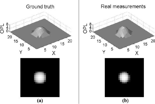
Optical Path Length (OPL) of a bead. (a) Ground truth OPL of the bead (the top and bottom illustrations show the surf view and 2D view of OPL, respectively); (b) Real measurement on beads' OPL from the restored phase contrast image.

The absolute error between the computed measurement and ground truth OPL (|OPL_{Real measurement} − OPL_{Ground truth}|) is shown in Figure 11(a). Over all pixel locations of the bead, the maximum absolute error is 1.06 pixel and the mean absolute error is 0.16 pixel, demonstrating the high accuracy of our restoration (Note: Since no sub-pixel technique is applied here, the highest achievable precision of an imaged-based measurement is 1 pixel.) From Figure 11(a), we also note that the maximum error occurs around a bead's peripheral regions. This is because of the more complex light diffraction and deflection around the peripheral regions compared to the inner microsphere regions. Figure 11(b) shows the OPL along the bead's middle horizontal profile. The thick solid black curve represents the ground truth OPL computed using the bead's mean diameter. The two thin solid black curves represent the ground truth OPL computed using the bead's mean diameter ± standard deviation. The band between the two thin solid black curves define the range of ground truth OPL on each pixel location (Note: The ground truth OPL has a standard deviation because of the imperfection of microsphere manufacturing.) The dashed and dash-dotted green curves in Figure 11(b) represent the mean and range of our OPL measurements on the beads. The two largely overlapping bands defined by the ground truth and our measurements prove that the OPL measurements from our imaging-model-based restoration is very close to the ground truth, thus validating our imaging model for the restoration procedure.

Figure 11.

Comparing our measurement with the ground truth. (a) The absolute error between the real measurement and ground truth OPL; (b) The OPL along the bead's middle horizontal profile.

Our imaging model for restoration depends on the hardware specifications of the phase contrast microscope such as the phase ring's outer radius (R) and ring width (W). For the phase contrast microscope that we used in this validation, R ≈ 6.1mm ≈ 4700pixels and W ≈ 1.2mm 900pixels. Figure 12 shows the mean absolute error between the computed measurements and ground truth OPL corresponding to the correct and wrong estimations of phase ring parameters. It turns out that wrong phase ring parameters do not generate satisfactory restoration results and the difference between the measured OPL and ground truth OPL is large. Understandably, the restoration achieves the least error when using the correct phase ring parameters (R ≈ 4700 and W ≈ 900 in this section) and it is stable around the correct parameters. There are strip patterns from northwest to southeast in the error matrix of Figure 12, the cause of which can be explained using Eq. 48 where the airy kernel (airy(r) = f_R(r)−f_R−W (r)) has two terms: $f_R\left(r\right)=R\frac{J_1\left(2\pi Rr\right)}{r}$ and $f_{R-W}\left(r\right)=(R-W)\frac{J_1\left(2\pi (R-W)r\right)}{r}$. When we change the parameters R and W with the same amount ∊, the first term of the airy kernel is changed but the second term is not since f_{R+∊−(W+∊)}(r) = f_R−W (r). Thus, the airy kernels are similar if we change a little on the R and use the same amount of change for W. Due to the similar airy kernels, the mean absolute error corresponding to different Rs and Ws within a local neighborhood is close. Consequently, the restoration is stable when there are small deviations on the phase ring parameters.

Figure 12.

The mean absolute error between real measurements and ground truth OPL regarding to di erent parameters on the phase ring (R and W ).

5.2. Restoration for Segmentation

Figure 13 shows several restoration samples on real phase contrast images. It appears that the restored artifact-free images are easier to be segmented because the cells are represented by bright (positive-value) pixels set on a uniformly black (zero-value) background. To see if this is the case, we have done quantitative evaluation of segmentation by using restored images in this section.

Figure 13.

Restored artifact-free phase contrast images. Top row: phase contrast microscopy images with increasing cell densities in the view field; Bottom row: the restorations corresponding to the top row.

Data

Two phase contrast microscopy image sequences were captured at the resolution of 1040 × 1392 pixels per image. Seq1: C2C12 muscle stem cells proliferated from 30+ to 600+ cells (imaged by ZEISS Axiovert 135TV phase contrast microscope at 5× magnification over 80 hours at 5 minute intervals, 1000 images in total, Figure 14(a,c)). Seq2: hundreds of bovine vascular cells migrated to the central image region (imaged by Leica DMI 6000B phase contrast microscope at 10× magnification over 16 hours at 5 minute intervals, 200 images in total, Figure 14(f,h)).

Figure 14.

Quantitative evaluation. (a–b, c–d, f–g, h–i): the pair of observed and restored images; (e): Ten ROC curves corresponding to ten annotated images in sequence 1; (f): Four ROC curves corresponding to four annotated images in sequence 2.

Parameters

We normalized the restored images onto value range [0, 1]. Based on a training pair of restored image and its ground truth mask (Seq1 uses the 500^th image and Seq2 uses the 100^th image), we applied a series of values between zero and one to threshold the restored image and compared them with the ground truth to compute TPR and FPR scores, which provided a ROC curve. Different parameter sets in the objective function generate different ROC curves. We searched the optimal parameter set (ω_s = 1, = ω_r = .001 and ω_t = .1 in the evaluation) with the largest area under the ROC curve (AUC). For the curve with the largest AUC, we searched the threshold that has the highest ACC to segment the restored image into a binary map (both Seq1 and Seq2 got the best threshold equal to 0.22). We applied the learned parameters to all other images.

Evaluation

We manually labelled every 100^th image in Seq1 (2369 annotated cell bitmasks in 10 images, 8.6 × 10⁵ cell pixels in total) and every 50^th image in Seq2 (2918 annotated cell bitmasks in 4 images, 1.1 × 10⁶ cell pixels in total). It took human experts about 2 hours to label one thousand cell bitmasks in an image. Figure 14 shows some input and restored images with all ROC curves of each individual image shown in Figures 14(e) and (j), where ROC curves deviate gradually from the perfect top-left corner (AUC=1) as cell density increases in the microscopy image sequence. The average AUC is 94.2% (Seq1) and 89.2% (Seq2), and the average segmentation accuracy is 97.1% (Seq1) and 90.7% (Seq2). We have achieved high segmentation accuracy that enabled accurate cell detection and tracking.

5.3. Comparison with Other Approaches

In this section, we compare our restoration-based segmentation with two other representative methods: (1) three-class Otsu thresholding (Figure 1(c)), which classifies pixels into inner dark cell regions, halo and background classes, and (2) level-set method, which evolves initial contours towards object boundaries. There are two common ways to define initial contours for the level-set approach: a single contour (Figure 15(a)) or multiple contours uniformly distributed over the entire image (Figure 15(b)). However, the evolution of contours from these two initializations stop around the halo regions as shown in the fourth column of Figures 15(a) and (b), which generate wrong segmentation. Another observation from Figures 15 (a) and (b) is that the level-set approach is sensitive to the initialization (e.g., the segmentation results in the fouth column of Figure 15 are different due to different initializations). For example, an initial contour inside a nucleus region will expand to the boundary between the nucleus and the halo. However, an initial contour containing the cell and halo will contract toward the boundary between the halo and the background, which does not provide satisfactory segmentation. For phase contrast images with halo artifact, the level-set approach works only when the initial contours are close to the evolution convergence, thus the third initialization we used is the segmentation of inner dark cell regions generated by the three-class Otsu thresholding method, as shown in Figure 15(c).

Figure 15.

Level set segmentation with three different initializations (Rows (a,b,c)). Column 1: Initialization (red contours) overlaid on the input image; Column 2: Binary mask corresponding to the initialization contours; Column 3: Evolved contour after 10000 iterations; Column 4: Segmentation mask corresponding to the evolved contours. For comparison, our segmentation is shown in Fig 19.

We compare our restoration-based segmentation with the Otsu thresholding method and level-set approach (initialized by segmentation of inner dark cell regions) on two microscopy image sequences (sequence 1 with 10 annotated images, sequence 2 with 4 annotated images). As shown in Figure 16, our approach outperforms the other two approaches consistently, based on the accuracy metric.

Figure 16.

Our restoration-based segmentation outperforms the Otsu thresholding and level-set approaches consistently, in terms of the accuracy metric. The top title summarizes the average accuracy of each method on the two sequences.

5.4. The Effects of Imaging Model and Regularizations on Restoration

Our linear imaging model (Eq. 18) indicates that the image formation process of phase contrast microscopy can be approximated by convolving an artifact-free image with a filtering kernel. Due to the convolution, a possible solution to restore the artifact-free image is blind-deconvolution (Levin et al., 2009), which estimates H and f at the same time. However, blind deconvolution might obtain an unsatisfactory result if the blindly estimated H does not correspond to the correct optics, as shown in Figure 17(c).

Figure 17.

The importance of imaging model and regularizations. (a) Input phase contrast image; (b) Restored image by our imaging model with smoothness and l₁ sparseness regularizations; (c) Blind deconvolution on the input phase contrast image; (d) Restored image without sparseness regularization; (e) Restored image without smoothness regularization.

We have developed regularized cost function (Eq. 28) to restore phase contrast images. When there is no sparse constraint, the restored image contains many false alarms from the background (Figure 17(d)). When there is no smoothness constraint, gaps between object parts, such as cell nuclei and membrane, may appear (Figure 17(e)).

To evaluate the effect of image-adaptive regularization, initialization from a look-up table, and temporal consistency on the restoration, we compare four different algorithm implementations on Seq1: (1) original restoration algorithm in Yin et al. (2010b) with constant sparseness matrix, constant initialization and without temporal consistency assumption; (2) revised Yin et al. (2010b) with regularization terms adapted to image properties (described in Section 4.3); (3) revised Yin et al. (2010b) with adaptable regularization terms and an initialization from a look-up table (described in Section 4.4); and, (4) revised Yin et al. (2010b) with all aforementioned techniques (image-adaptive regularization, initialization from a look-up table, and temporal consistency assumption).

Seq1 includes a growing number of stem cells (Figure 14(a,c)). When the cell number increases, the image has more nonnegative f values (cell pixels) and this causes more element-wise computation in Eq. 33, therefore the computational cost increases from the beginning to the end of this sequence, as shown in Figure 18(a). From Figure 18(a), we also observe that all the proposed techniques (image-adaptive regularization, initialization from a look-up table and temporal consistency assumption) have contributed to decrease the computational cost. As the cell number increases in the sequence, the restoration accuracy decreases a little bit as shown in Figure 18(b), because a large number of cells cultured in the dish may occlude each other and blur the halo effect. Furthermore, from Figure 18(b), we observe the four algorithm implementations have similar accuracies compared to each other. The reason is because our numerical iterative algorithm to solve the nonnegative quadratic optimization problem in Eq. 30 is guaranteed to converge to a unique global optimum (Sha et al., 2007), which is an appealing property.

Figure 18.

Comparing four algorithm implementations on restoring every 100th image of a phase contrast microscopy image sequence, in terms of time cost and segmentation accuracy.

5.5. Restoration for Cell Detection and Tracking

The restored phase contrast images have attractive properties such that cell pixels have positive values on a uniformly zero-value background, which can greatly facilitate the cell detection and tracking task. Given a phase contrast image (Figure 19(a)), we restore it (Figure 19(b)) and threshold the result to get the bitmap, shown in Figure 19(c). We connect the bright pixel components into blobs (cell candidates) and classify the blobs into cells or non-cells using a trained SVM classifier (Cristianini and Shawe-Taylor, 2000). The blob features we used in the SVM classifier include blob area, shape and corresponding intensity values in the phase contrast image and the restored image. Figure 19(d) shows the classification result and Figure 19(e) shows the detected cells overlaid on the original image. Compared to the segmentation results using traditional image processing methods in Figure 1, our restored artifact-free image is much easier for segmenting and detecting cells. For qualitative evaluation, Figure 20 shows more cell detection results based on restored phase contrast images. The overlapping/occluding cells can be handled by the algorithm in (Bise et al., 2009) that matches partial contours of overlapping cells to maintain cell identities.

Figure 19.

Segment and detect cells based on the restoration result. (a) Input phase contrast image; (b) Restored artifact-free image; (c) The bitmap by thresholding the restored image; (d) The blobs classified as cells; (e) The detected cells overlaid on the original image with cell contours (red) and cell IDs(green).

Figure 20.

Top row: input phase contrast images; Middle row: restored phase contrast images; Bottom row: detected cells are labelled by red boundaries and green IDs.

We quantitatively evaluate the performance of cell detection using a fully annotated sequence from (Kanade et al., 2011) where a total of 85, 681 cell centroids are annotated in 780 images. Denoting annotated cells as positive (P), the Recall of detection is defined as Recall = |TP|/|P|, where true positive (TP) stands for those cells correctly detected by both skilled human our method and our method, and the Precision is defined as Precision = |TP|/(|TP| + |FP|), where false positives (FP) are those cells detected by mistakenly. Over the 85, 681 cells in 780 images, we achieve Precision of 91% and Recall of 90%. The cell detection module based on our restoration method is integrated into a large-scale cell tracking system that has been applied to several biological applications such as stem cell production and wound healing assays (Kanade et al., 2011).

There are a few failure cases in cell detection. As shown in Figure 21, the false positives are mainly from dirt in the background or extended cell structures with positive values in the restored image. We believe a cell classifier using temporal context may overcome this problem and plan to explore that in the future work. Most of the missed cell detections come from cell mitosis (cell division) regions because these regions do not follow the normal cell appearance model. The mitotic cells are bright regions instead of dark cell regions surroundded by bright halos. We use mitosis event detection methods (e.g., Liu et al. 2010) to detect these mitotic cells for cell tracking applications.

Figure 21.

Evaluate the performance of cell detection based on restoration. (a,c) Input phase contrast image with the detected cells compared to the ground truth. (b,d) The restored phase contrast image.

6. Conclusion

The halo and shade-off artifacts in phase contrast microscopy hinder automated microscopy image analysis such as cell segmentation, a critical step in cell tracking systems. We derived a linear imaging model representing the optical properties of phase contrast microscopes. Using this model, we develop an algorithm to restore artifact-free phase contrast images by solving a regularized quadratic optimization problem. The regularization terms are adapted to input image properties and we consider temporal consistency when restoring time-lapse microscopy images. To accelerate the iterative process, we infer an initialization close to the optimal solution by using a lookup table built from training images. The restored artifact-free images are amenable to cell segmentation via thresholding. This work suggests that understanding the optics of microscopes can lead to more proficient microscopy image analysis and interpretation. In particular, we have demonstrated that this approach can greatly facilitate cell segmentation, detection and tracking.

• Understand the phase contrast optics and its artifacts

• Derive the computational imaging model for phase contrast optics

• Design an effective algorithm to restore artifact-free phase contrast images

• Facilitate high-performance microscopy image analysis such as cell segmentation

Appendix I: Derivation on Eq. 15

The inverse Fourier transform of T_D(·) (Eq. 8) is derived based on the Hankel transform (The inverse 2D Fourier transform of a circularly symmetric function is known as the zero-order Hankel transform (Gaskill, 1978)). The zero-order Hankel transform on a cylinder function is

$${\mathcal{H}}_0:\text{cyl}\left(t\right)\leftrightarrow \pi \text{somb}\left(r\right)$$ (45)

where $r=\sqrt{u^2+v^2}$ is the radial distance and somb(·) is the sombrero function (resembles a Mexican hat)

$$\text{somb}\left(r\right)=\frac{2J_1\left(2\pi r\right)}{2\pi r}$$ (46)

and J₁(·) is the first order Bessel function of the first kind. Applying the zero-order Hankel transform (Eq. 45) onto T_D(·), we get

$$t_D\left(\mathbf{x}\right)=\delta \left(\mathbf{r}\right)+(i{\zeta }_p-1)\text{airy}\left(r\right)$$ (47)

where airy(r) is an obscured Airy pattern (Born and Wolf, 1997)

$$\text{airy}\left(r\right)=R\frac{J_1\left(2\pi Rr\right)}{r}-(R-W)\frac{J_1\left(2\pi (R-W)r\right)}{r}.$$ (48)

Appendix II: Derivation on Eq. 18

First, we normalize the Airy kernel

$$\text{airy}\left(\mathbf{r}\right)\leftarrow \frac{\text{airy}\left(\mathbf{r}\right)}{1\ast \text{airy}\left(\mathbf{r}\right)}$$ (49)

such that any constant matrix convolved with the normalized airy(·) will be the constant matrix itself. Secondly, the Taylor expansion of e^−if(x) is

$$e^{-if\left(\mathbf{x}\right)}=1-if\left(\mathbf{x}\right)+\frac{{\left(if\left(\mathbf{x}\right)\right)}^2}{2!}+\cdots$$ (50)

Since the phase shift caused by the specimen is small, the higher order terms are close to zero, i.e.

$${\left(f\left(\mathbf{x}\right)\right)}^2\approx 0$$ (51)

Based on Eqs. 49 and 51, we have

$${(f\left(\mathbf{x}\right)\ast \text{airy}\left(\mathbf{r}\right))}^2\approx 0$$ (52)

Based on Eqs. 50 and 51, we have

$$e^{-if\left(\mathbf{x}\right)}\approx 1-if\left(\mathbf{x}\right).$$ (53)

Using Eqs. 51, 52 and 53, we compute the intensity of an observed image as

$$g\left(\mathbf{x}\right)=\mid {\tilde{l}}_S\left(\mathbf{x}\right)-{\tilde{l}}_D\left(\mathbf{x}\right){\mid }^2$$ (54)

$$=\mid i{\zeta }_{p}A{e}^{i\beta }-{\zeta }_{c}A{e}^{i(\beta -f\left(\mathbf{x}\right))}-(i{\zeta }_p-1){\zeta }_{c}A{e}^{i(\beta -f\left(\mathbf{x}\right))}\ast \text{airy}\left(r\right){\mid }^2$$ (55)

$$\approx 2{\zeta }_c{\zeta }_p{A}^2\left(\frac{{\zeta }_p{(1-{\zeta }_2)}^2}{2{\zeta }_c}+f\left(\mathbf{x}\right)-f\left(\mathbf{x}\right)\ast \text{airy}\left(\mathbf{r}\right)\right)$$ (56)

$$\propto C+f\left(\mathbf{x}\right)\ast (\delta \left(\mathbf{r}\right)-\text{airy}\left(\mathbf{r}\right))$$ (57)

where $C=\frac{{\zeta }_p{(1-{\zeta }_c)}^2}{2{\zeta }_c}$ is a constant.

References

- Bise R, Li K, Eom S, Kanade T. Reliably Tracking Partially Overlapping Neural Stem Cells in DIC Microscopy Image Sequences. Proceedings of MICCAI workshop on Optical Tissue Image Analysis in Microscopy, Histopathology and Endoscopy (OPTMHisE); London, UK. 2009. pp. 67–77. [Google Scholar]
- Born M, Wolf E. Principles of Optics. sixth ed. Pergamon Press; 1980. [Google Scholar]
- Candes E, Wakin M, Boyd S. Enhancing Sparsity by Reweighted l1 Minimization. The Journal of Fourier Analysis and Applications. 2008;14(5):877–905. [Google Scholar]
- Cristianini N, Shawe-Taylor J. An Introduction to Support Vector Machines and Other Kernel-based Learning Methods. first ed. Cambridge University Press; 2000. [Google Scholar]
- Gaskill J. Linear Systems, Fourier Transforms, and Optics. Wiley; 1978. [Google Scholar]
- House D, Walker ML, Wu Z, Wong JY, Betke M. Tracking of Cell Populations to Understand their Spatio-Temporal Behavior in Response to Physical stimuli. Proceedings of Workshop on Mathematical Modeling in Biomedical Image Analysis (MMBIA); Miami, FL, USA. 2009. pp. 186–193. [Google Scholar]
- Kanade T, Yin Z, Bise R, Huh S, Eom S, Sandbothe M, Chen M. Cell Image Analysis: Algorithms, Systems and Applications. Proceedings of IEEE Workshop on Applications of Computer Vision (WACV); Kona, HI, USA. 2011. pp. 374–381. [Google Scholar]
- Kim S-J, Koh K, Lustig M, Boyd S, Gorinevsky D. An Interior-Point Method for Large-Scale l1-Regularized Least Squares. IEEE Journal of Selected Topics in Signal Processing. 2007;1(4):606–617. [Google Scholar]
- Levin A, Weiss Y, Durand F, Freeman WT. Understanding and Evaluating Blind Deconvolution Algorithms. Proceedings of IEEE Conference on Computer Vision and Pattern Recognition (CVPR); Miami, FL, USA. 2009. pp. 1964–1971. [Google Scholar]
- Li K, Miller ED, Chen M, Kanade T, Weiss L, Campbell PG. Cell Population Tracking and Lineage Construction with Spatiotemporal Context. Medical Image Analysis. 2008;12(5):546–566. doi: 10.1016/j.media.2008.06.001. [DOI] [PMC free article] [PubMed] [Google Scholar]
- Li K, Kanade T. Nonnegative Mixed-Norm Preconditioning for Microscopy Image Segmentation. Proceedings of the 21st International Conference on Information Processing in Medical Imaging (IPMI); Williamsburg, VA, USA. 2009. pp. 362–374. [DOI] [PubMed] [Google Scholar]
- Liu A, Li K, Kanade T. Mitosis Sequence Detection Using Hidden Conditional Random Fields. Proceedings of IEEE International Symposium on Biomedical Imaging (ISBI); Rotterdam, Netherlands. 2010. pp. 580–583. [Google Scholar]
- Meijering E, Dzyubachyk O, Smal I, Cappellen WA. Tracking in Cell and Developmental Biology. Seminars in Cell and Developmental Biology. 2009;20(8):894–902. doi: 10.1016/j.semcdb.2009.07.004. [DOI] [PubMed] [Google Scholar]
- Murphy D. Fundamentals of Light Microscopy and Electronic Imaging. Wiley; 2001. [Google Scholar]
- Otsu N. A Threshold Selection Method from Gray-Level Histograms. IEEE Trans. on Systems, Man, and Cybernetics. 1979;9(1):62–66. [Google Scholar]
- Rittscher J. Characterization of Biological Processes through Automated Image Analysis. Annual Review of Biomedical Engineering. 2010;12:315–344. doi: 10.1146/annurev-bioeng-070909-105235. [DOI] [PubMed] [Google Scholar]
- Sha F, Lin Y, Saul L, Lee D. Multiplicative Updates for Nonnegative Quadratic Programming. Neural Computation. 2007;19(8):2004–2031. doi: 10.1162/neco.2007.19.8.2004. [DOI] [PubMed] [Google Scholar]
- Smith K, Carleton A, Lepetit V. General Constraints for Batch Multiple-Target Tracking Applied to Large-Scale Video Microscopy. Proceedings of IEEE Conference on Computer Vision and Pattern Recognition (CVPR); Anchorage, AK, USA. 2008. p. 8. [Google Scholar]
- Wu K, Gauthier D, Levine M. Live Cell Image Segmentation. IEEE Trans. on Biomedical Engineering. 1995;42(1):1–12. doi: 10.1109/10.362924. [DOI] [PubMed] [Google Scholar]
- Yang F, Mackey MA, Ianzini F, Gallardo G, Sonka M. Cell Segmentation, Tracking, and Mitosis Detection Using Temporal Context. Proceedings of the 8th International Conference on Medical Image Computing and COmputer Assisted Intervention (MICCAI); Palm Springs, CA, USA. 2005. pp. 302–309. [DOI] [PubMed] [Google Scholar]
- Yin Z, Bise R, Kanade T, Chen M. Cell Segmentation in Microscopy Imagery Using a Bag of Local Bayesian Classifiers. Proceedings of IEEE International Symposium on Biomedical Imaging (ISBI); Rotterdam, Netherlands. 2010. pp. 125–128. [Google Scholar]
- Yin Z, Li K, Kanade T, Chen M. Understanding the Optics to Aid MIcroscopy Image Segmentation. Proceedings of the 13th International Conference on Medical Image Computing and Computer Assisted Intervention (MICCAI); Beijing, China: 2010. pp. 209–217. [DOI] [PubMed] [Google Scholar]
- Yin Z, Kanade T. Restoring Artifact-free Microscopy Image Sequences. Proceedings of IEEE International Symposium on Biomedical Imaging (ISBI); Chicago, IL, USA: 2011. pp. 909–913. [Google Scholar]
- Zernike F. How I discovered phase contrast. Science. 1955;121:345–349. doi: 10.1126/science.121.3141.345. [DOI] [PubMed] [Google Scholar]