Different tests for a difference: how do we do research?

Key points

• Frequentist probability concerns the possibility of NO difference

• The starting premise is a population with known features

• Bayes’ theories concern modifying a pre-existing possibility

• Experiments revise the previous estimate

• Lab experiments do not often use random samples

• Small numbers, random allocation to treatment

• Well suited to permutation tests

• Choose the test when you devise the experiment

• Make sure that the equipment (and the test) are appropriate

Most biological scientists conduct experiments to look for effects and test the results statistically. We have already described Student's t-test, which is very commonly used. However, this test concentrates on a very limited question. We assume that there is no effect in the experiment, and then estimate the possibility that we could have obtained these results. The question concerns what we may deduce, if the samples measured came from a single theoretical population of known characteristics. We calculate the probability that we might obtain the results we did, or more extreme results, on the basis of this premise. The statistical procedure is called frequentist because the results are expressed in terms of ‘how frequently would a result like this be observed, given the exact definition of the theoretical population that we proposed?’ (Figure 1).

Figure 1.

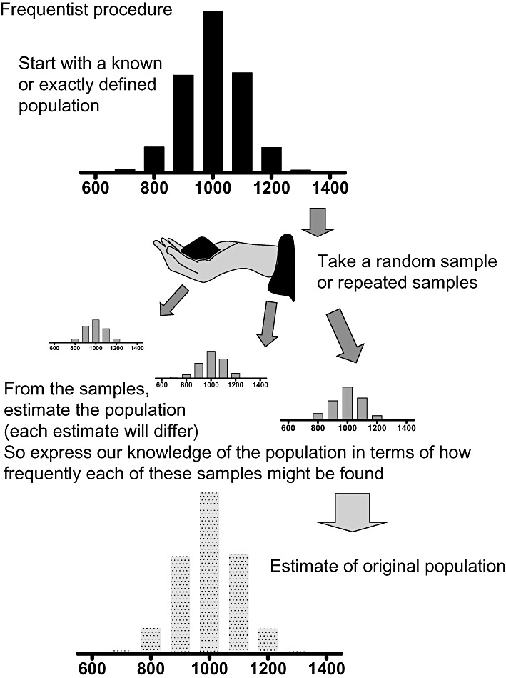
The frequentist approach considers the result of taking multiple samples from a known population. The P value is the probability of obtaining such samples, if it were the same population that had been sampled, each time. The samples provide estimates of the original population.

The logic of the Student's t-test procedure, which is a null hypothesis significance test, is not very clear when applied to biological experiments, which are usually done to show effects. The Student's t-test proposes that we are NOT going to find an effect. We then express the results of our study based on this premise of no effect, as the probability of obtaining the results we have obtained, if the samples were taken from the same population. In formal terms, we use the testing process to calculate the probability P of obtaining these data, given the proposed hypothesis of no effect (H₀).

Put into relatively plain English, we ask how well (expressed as a probability) do the observations (data) support this possibility (H₀). What we are looking for is a lack of support, because we are never going to find NO difference at all between samples, simply because of random variation. To be absolutely fair to this process, we are using this ‘straw man’ as a model for comparison, rather than an actual suggestion of reality. What we cannot infer is that if we find a lack of support, then the converse is likely. We cannot turn the probability round and argue that from our knowledge of how little support there is, we then know how probable it is that the null hypothesis is true. In other words, we do not obtain the probability of the truth of the null hypothesis, given the data:

In fact, the null hypothesis is never true, in absolute terms. A sufficiently large experiment would always find some evidence against the null hypothesis. Biologists, and others, are more likely to ask different questions of their data, such as what is the probability that when they apply a treatment, it will yield a particular effect of biological interest. Formally, what is the probability of an effect, given the data that are observed?

Is there an alternative to testing the null hypothesis? Probably not directly. Cohen (1994) summarized the arguments of many of the previous voices raised against null hypothesis tests, and advised: ‘First, don't look for a magic alternative to null hypothesis testing, some other objective mechanical ritual to replace it. It doesn't exist.’ If this is so, then what approaches can be used?

We can refine the process of classical statistical reasoning, using more thoughtful processes. Testing the null hypothesis should not be carried out in isolation. We could try an application of MAGIC, an acronym introduced by Abelson who argues that a research result should be subject to a basket of assessment criteria: Magnitude, Articulation of effect, Generality, Interestingness and Credibility (Abelson, 1995). The P value can be used, in different situations, to assess both credibility and generality. We can also use confidence intervals to provide a stronger idea of the magnitude of effect.

An alternative analysis is suggested by a common feature of most biological experiments. We may already have some idea of the expected outcome, and the results can be used to confirm or deny these predictions. This is a Bayesian approach to data analysis, using observed results to modify or support the supposed outcome (Figure 2). To express this question statistically, we ask ‘How do the data modify our prediction of the effects of this intervention?’ To take this approach, a prior possibility, or distribution, has to be predicted. This prediction may be based on the experimenter's educated guess, or the opinion of a group of experts, or it could more likely have come from a series of preceding experiments, to obtain some idea of the possible population. The experimental data are then used to modify the prior distribution. When this process is complete, we generate a revised estimate of the population values, which is the posterior distribution. The effects are often expressed in terms of the ‘credible interval’ to quantify the population parameter. This is a concept similar to a confidence interval. This approach uses the experimental data to more accurately define a population, and the credible interval indicates where the possible population parameter is likely to be found. In contrast, the classical hypothesis testing model takes the premise that the population parameters have fixed values, and that our uncertainty is how well we can estimate where the value lies. The confidence interval (for example the 95% confidence interval) is a range that will vary with each sample taken from the population, but is likely, in the long run, to contain the true population value in 95% of estimates based on repeated samples from the population. This difference is subtle but real. A reasonable analogy could be looking for a lost mobile telephone. The credible interval is that it is likely to be in a particular room, so that is where I would go first (it is here somewhere): the confidence interval is that it is definitely in one place (it has to be somewhere) but my chance of going to the correct room each time I go to look for it is not 100%!

Figure 2.

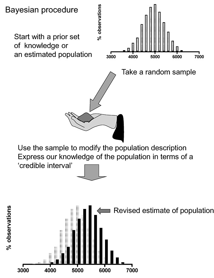
The Bayesian approach is to take a sample that is used to allow further information about the original, not so well-characterized population: the test results give a more firm measure of the original.

An approach to testing which is well suited to the usual pattern of lab experiments is the permutation test (also known as randomization tests, rerandomization tests or exact tests). As Ludbrook and Dudley (1998) showed very well, the vast majority of lab studies are not based on random samples from populations, as the Student's t-test supposes. In contrast, the usual lab experiment uses a small set of material (animals, organs, cells, proteins) divided randomly into groups that are allocated different treatments. By using the data from the entire population at our disposal, we need not make assumptions about sampling from populations. With such conditions, the permutation test could be a better choice than the Student's t-test (Ludbrook and Dudley, 1998; Lew, 2008). A permutation test estimates the probability of arrangements of values within the data observed (Figure 3). This is expressed as the number of ways that the data can be arranged that would generate a difference equal to or greater than (at least as extreme as) the difference actually observed, as a fraction of the total possible number of arrangements. The null hypothesis is to consider that the disposition of the data values we have obtained would be distributed randomly between the groups, which would be true if the treatment caused no effect. This hypothesis differs substantially from that of the t-test; and the result naturally reflects the values in the sample tested, not a theoretical general population. The implicit assumption is that the sample used can be representative of a larger population: this is not necessarily always a valid assumption to make. As an illustration, in the example we consider later, it could be that some animal colonies have bedding that contains lots of rubidium, which makes up for what the diet lacks.

Figure 3.

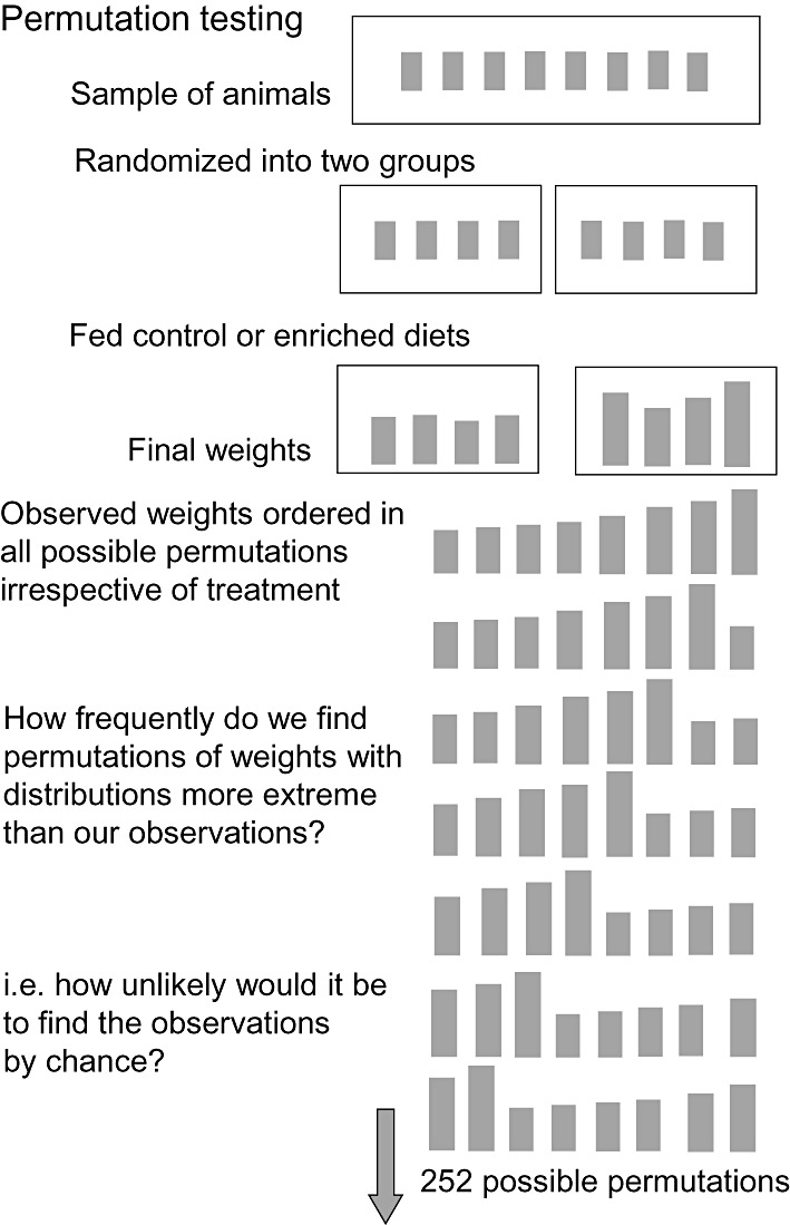
The permutation test assembles the observed experimental data in all possible arrangements. Each arrangement would be equally possible if the allocation of data were random. We can then assess the likelihood of the data being distributed the way they have been found to occur.

Consider two groups of animals, drawn from a laboratory colony of 10, with a diet (and bedding) considered to be deficient in rubidium. These animals are randomly allocated to continue with their previous (control) diet or to be fed a diet enriched with rubidium. After 6 weeks, their weights (in g) are:

Control diet	23	30	28	31	26
Rubidium diet	37	34	29	33	32

We propose that the weights could have come from a single population, and that any distribution of these values would be random between Control and Rubidium diets. In other words, if we put these numbers into one set, and then separate them into two groups of five, how many different arrangements would result? Working systematically, we could start by ranking the numbers from least to greatest. Thus one arrangement of the numbers could be:

Control	23	26	28	29	30
Rubidium	31	32	33	34	37

Here, the numbers are arranged in sequence from the least to the greatest. The next most extreme would be:

Control	23	26	28	29	31
Rubidium	30	32	33	34	37

There is a formula for this process, based on the factorial for the component numbers. (The factorial of the positive integer n is the product of all positive integers less than or equal to n, so 5! = 5 × 4 × 3 × 2 × 1.).

In our example, the number of different combinations is given by

This shows that there are 252 possible ways to arrange these numbers into two separate groups. If we count the number of sequences, we can construct that are as extreme or more extreme, in both directions, than the observed data, we find there are eight such sequences. Thus, the possibility of these sequences is eight out of 252, and 8/252 is 0.032, and thus we have a two-sided P of 0.03. Therefore, we might conclude that there is likely to be a difference in mean weight between the two groups.

This test is reliable even when the data are not normally distributed (a requirement of the t-test), but it is only easy to calculate when the sample sizes are small, because the number of possible permutations of a set of numbers increases very rapidly as the set gets bigger. When the sample is large, the process of the test can be speeded up by taking a random sample of the permutations. With small sample sizes (a number of permutations less than 20), a probability less than 0.05 cannot be attained, but this is possible with two independent groups of four, or related groups with more than five. When groups of this size are tested there may be problems with other statistical tests such as the Wilcoxon–Mann–Whitney (aka the Wilcoxon two-sample or rank sum or Mann–Whitney U) test, and the permutation test is ideal for these small groups. Ludbrook and Dudley (1998) suggest a number of sources of testing procedures and Lew provides software at http://www.pharmacology.unimelb.edu.au/statboss/home.html.

Other suitable software can be found in packages such as StatXact or R, and packages such as SAS and SPSS contain permutation modules from StatXact.

An alternative approach that often suits biological data from experiments very well is to construct a model, for example using a linear or logistic regression to explain the data, and see how well the model fits. A simple example would be a dose–response curve. For scientists who are investigating mechanisms, this process is very satisfactory, and we will consider this approach more closely in a later paper.

In conclusion, statistical tests are tools to be used carefully and with some prior thought. Unless you were very good at do-it-yourself, you would be unwise to choose from the pages of a modern tool catalogue without advice, and the same is true of statistics. Get the right tool, and after a little instruction, you are set for the job in hand, or better still, for the job you are planning.

Conflict of interest

None.

References

- Abelson RP. Statistics As Principled Argument. Erlbaum: Mahwah, N.J; 1995. [Google Scholar]
- Cohen J. The earth is round (p < .05) Am Psychol. 1994;49:997–1003. [Google Scholar]
- Lew MJ. On contemporaneous controls, unlikely outcomes, boxes and replacing the ‘Student’: good statistical practice in pharmacology, problem 3. Br J Pharmacol. 2008;155:797–803. doi: 10.1038/bjp.2008.350. [DOI] [PMC free article] [PubMed] [Google Scholar]
- Ludbrook J, Dudley H. Why permutation tests are superior to t- and F-tests in biomedical research. Am Stat. 1998;52:127–132. [Google Scholar]