Competing risks regression for clustered data

Abstract

A population average regression model is proposed to assess the marginal effects of covariates on the cumulative incidence function when there is dependence across individuals within a cluster in the competing risks setting. This method extends the Fine–Gray proportional hazards model for the subdistribution to situations, where individuals within a cluster may be correlated due to unobserved shared factors. Estimators of the regression parameters in the marginal model are developed under an independence working assumption where the correlation across individuals within a cluster is completely unspecified. The estimators are consistent and asymptotically normal, and variance estimation may be achieved without specifying the form of the dependence across individuals. A simulation study evidences that the inferential procedures perform well with realistic sample sizes. The practical utility of the methods is illustrated with data from the European Bone Marrow Transplant Registry.

1. INTRODUCTION

Competing risks regression was proposed by Fine and Gray (1999) to assess the effects of covariates on the probabilities of a particular cause of failure with independent subjects, where each subject may fail from one of several causes. Naively, censoring subjects who fail from causes other than that of interest may yield an invalid analysis for the cumulative probabilities of the cause of interest across time. The Fine and Gray (1999) regression model, which is specified for the cumulative incidence, treats the competing causes differently from independent censoring variables and has been adopted in practice as an alternative to the naive analysis described above.

In many applications involving competing risks, individuals may be correlated within clusters, owing to unobserved shared factors across individuals. We refer to such data as “clustered competing risks,” with “clustering” referring to the potential dependence across individuals within clusters and “competing risks” referring to the potential dependence across causes within individuals, analogously to the case of independent subjects (Fine and Gray, 1999). In family studies of hereditary cancer, parents and children may share genetic and environmental factors, leading to familial correlations in disease onset. In multicenter studies, patient population and referral pattern in each center may result in correlated outcomes within centers. The current work extends the Fine and Gray (1999) model to this clustered setup.

Numerous semiparametric regression models have been proposed for the clustered data setting with independent censoring but without dependent competing risks. Wei and others (1989) proposed a proportional hazards model with common covariate effects but different baseline hazard for each cluster member. Lee and others (1992), Liang and others (1993), and Cai and Prentice (1997) studied proportional hazards models with common baseline and regression coefficients. These marginal models are specified unconditionally, with both the regression coefficients and the baseline hazards having population average interpretations. Inferences for the marginal regression models are generally robust to assumptions about the within-cluster correlations. To investigate the covariate effects conditionally on cluster, frailty models may be employed (Clayton and Cuzick 1985; Hougaard 1986). These conditional models involve explicit assumptions on the within-cluster dependence, enabling an assessment of both covariate effects and within-cluster associations.

For clustered competing risks, one may employ methods for independently censored data described above in the analysis of the cause-specific hazard functions (Prentice and others, 1978). These methods are not generally appropriate for the cumulative incidence function. Existing methods for the cumulative incidence with clustered data include a random effects Fine–Gray model specified conditionally on cluster authorGray:1988's (1988) test (Chen and others, 2008), which is applicable with categorical covariates. If the main goal is formulating a cumulative incidence regression model to investigate the effects of covariates, introducing a dependence parameter to model associations within individuals in a cluster does not seem to have much advantage over a marginal modeling strategy, in which the dependence is unspecified.

In this article, we propose to extend the Fine–Gray model to the clustered data setting, so that the cumulative incidence function can be estimated by adjusting for prognostic factors while accommodating correlation within clusters. We construct a marginal proportional subdistribution hazards model, which is similar to the Lee and others (1992) marginal model except that we focus on subdistribution hazards instead of cause-specific hazards. Under an independence working assumption, the cumulative incidence function and the effects of the prognostic factors can be estimated by following the Fine–Gray methodology. The proposed variance estimator accommodates the correlation within clusters. Ad hoc approaches to such marginal competing risks models might be utilized, with Ruan and Gray (2008) and Logan and others (2011) employing imputation and pseudovalues at discrete time points, respectively. However, the current study is the first to formally investigate inferential issues.

Section 2 introduces the marginal Fine–Gray model for clustered data. In Section 3, we discuss partial likelihood inferences for the marginal model, as well as inverse weighted estimating equations, which permit independent censoring from loss to follow-up in addition to the potentially dependent competing risks. Such inverse weighting methods are nonstandard, as they involve estimating the censoring probabilities using clustered censoring times, which may be correlated. Asymptotic properties of the estimators are established, along with a simple plug-in variance estimator. Section 4 assesses the performance of the proposed model through simulation studies, with the analysis of the motivating data following in Section 5. We conclude with a few remarks. The technical details are included in the supplementary material available at Biostatistics online.

2. MARGINAL PROPORTIONAL SUBDISTRIBUTION HAZARDS MODEL

Let T _ik be the failure time for the kth member in the ith cluster, i = 1,…,n;k = 1,…,m _i. Let ε_ik∈{1,…,l} denote the corresponding cause of failure and Z _ik = {Z _1ik,…,Z _pik} be a p×1 vector of covariates. For right-censored data, one observes {X _ik = T _ik∧C _ik,ξ _ik = I(T _ik ≤ C _ik)ε_ik,Z _ik}, where C _ik is the independent censoring time, ξ _ik∈{0,1,…,l}, and a∧b = m i n (a,b). The covariates Z _ik may include time-varying components, which are known deterministic functions of time and/or time-independent components, hence fully observed. The dependence on time is suppressed where possible, to ease readability.

We assume that (T _ik,ε_ik) and C _ik are independent given Z _ik for each i and k. Let T _i = (T _i1 ,…,T _imi), ε_i = (ε_i1 ,…,ε_imi), Z _i = (Z _i1 ,…,Z _imi), and C _i = (C _i1 ,…,C _imi). We assume that (T _i,ε_i,Z _i,C _i,m _i)_{i = 1,…,n} are i.i.d. We also require that (T _i,ε_i) and C _i are independent given (Z _i,m _i). In cluster i, the components of (T _i,ε_i) may be correlated conditionally on (Z _i,m _i), and similarly, the components of C _i may be dependent conditionally on (Z _i,m _i). Let X _i = (X _i1 ,…,X _imi) and ξ _i = (ξ _i1 ,…,ξ _imi). The observed data within each cluster, (X _i,ξ _i,Z _i,m _i), are assumed to be i.i.d. across clusters i = 1,…,n.

We are interested in assessing the effects of covariates on the marginal cumulative incidence function for failure from cause 1, conditional on the covariates: F ₁(t;Z _ik)≡P r(T _ik ≤ t,ε_ik = 1|Z _ik). The marginal subdistribution hazard λ ₁(t;Z _ik) = d F ₁(t;Z _ik)/{1 − F ₁(t;Z _ik)} is modeled as

(2.1)

where λ ₁₀(·) is a completely unspecified baseline subdistribution hazard function and β ₀ is a p×1 vector of unknown regression parameters. As in Fine and Gray (1999), our methodology does not require any assumptions regarding the cumulative incidence functions for other causes. As noted in Fine and Gray (1999), there is potential to gain efficiency by adding such assumptions but with greatly increased computational and theoretical challenges. Moreover, our analyses of model (2.1) will not be affected by whether we treat all competing causes {2,…,l} separately or group them. It is worth emphasizing that independent censoring by C enters differently into the analysis than the competing events and cannot be grouped with competing causes.

3. ESTIMATION AND INFERENCE

3.1. Censoring complete data

The term censoring complete (CC) data refers to the case in which failure time T is right censored but potential censoring time C is always observed, that is, censoring results only from administrative loss to follow-up. We modify the partial likelihood of Fine and Gray (1999) to accommodate clustering via an independence working assumption. The case of complete data where C is larger than the maximal failure time, that is, all event times and types are observed, is a special case of this setup. Hereafter, it is assumed that there exists a τ such that P(T _ik > τ) > δ > 0,P(C _ik = τ) = P(C _ik ≥ τ) > δ > 0 for all i,k.

Let N _ik(t) = I(T _ik ≤ t,ξ _ik = 1) and Y _ik(t) = 1 − N _ik(t − ) denote the counting process and risk process for the complete data, respectively. When the data are CC, the risk process is modified to Y _ik ^*(t) = I(C _ik ≥ t)Y _ik(t).

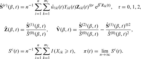
For convenience, we define the following notation:

where a ^⊗0 = 1,a ^⊗1 = a, and a ^⊗2 = a a ^T. The following regularity conditions are needed:

Assumption 3.1 Regularity conditions assumed throughout:

A1. ∫₀ ^τ λ ₁₀(t)dt < ∞.

A2. Z _pik(·) have bounded total variations, that is, |Z _pik(0)| + ∫₀ ^τ|dZ _pik(t)| ≤ M for all p, i, and k, where M is a constant.

A3. There exists a neighborhood ℬ of β ₀ and scalar, vector, and matrix functions s ⁽⁰⁾, s ⁽¹⁾, and s ⁽²⁾, defined on ℬ×[0,τ] such that for r = 0,1,2, sup_{t∈[0,τ],β∈ℬ}‖S ^(r)(β,t) − s ^(r)(β,t)‖ converges in probability to zero.

A4. s ^(r)(β,t) are continuous functions of β∈ℬ uniformly in t∈[0,τ] and are bounded on ℬ×[0,τ]. s ^(r)(β,t) are bounded away from zero.

A5. The matrix Ω = ∫₀ ^τ v(β ₀,u)s ⁽⁰⁾(β ₀,u)λ ₁₀(u)du is positive definite.

Under the independence working assumption, the pseudopartial likelihood (Lee and others, 1992) for β ₀ is

with corresponding estimating function

(3.1)

The estimator $\widehat{\beta }$ that maximizes L ^*(β) may be obtained as a solution to U ₁ ^*(β) = 0. The asymptotic results for CC data estimation are natural extensions of those from the ordinary Cox-type model for clustered data (Lee and others 1992; Spiekerman and Lin 1998). We present the main results briefly, as a point of comparison for subsequent results where inverse weighting is needed. In the supplementary material available at Biostatistics online, the estimator $\widehat{\beta }$ is shown to be consistent and asymptotically normal, with variance which may be consistently estimated using a sandwich variance estimator, which is robust to the within-cluster correlations. The form of the variance estimator is essentially identical to that in Lee and others (1992), with a minor modification for the censoring time always being observed.

3.2. Right-censored data

When the data are right censored, inverse probability of censoring weighting (Robins and Rotnitzky, 1992) techniques cannot be applied directly, owing to correlation within clusters. To account for such clustering, we define a marginal inverse probability of censoring weight for subject k in the ith cluster at time t. As in Fine and Gray (1999), we assume that C _ik is independent of Z _ik, with the weight w _ik(t)≡I(C _ik ≥ T _ik∧t)G(t)/G(X _ik∧t), where G(t) = P r(C _ik ≥ t).

Since the cluster sizes are finite, we cannot consistently estimate the censoring distribution in each cluster. Hence, we pool across cluster via the assumption of a single G. Note that the independent censoring times may be correlated within a cluster, but that data are uncorrelated across clusters.

We naively estimate G(·) with $\widehat{G}(·)$, the Kaplan–Meier estimator of the survival function of the censoring random variable in which the dependence among individuals within clusters is ignored. The estimated weight ${\widehat{w}}_{ik}\left(t\right)=I(C_{ik}\ge T_{ik}\wedge t)\widehat{G}\left(t\right)/\widehat{G}(X_{ik}\wedge t)$ is used in place of w _ik(t) in the estimating equation. In the case where m _i = 1;i = 1,…,n, this approach is equivalent to that in Fine and Gray (1999).

In addition to the notation in Section 3.1, the following notation is needed.

The inverse weighted estimating equation is

(3.2)

where M _ik(β,t) = ∫₀ ^tdN _ik(t) − ∫₀ ^t Y _ik(u)λ ₁₀(u) e ^β′Z_ik(u) d u is a martingale for marginal complete data filtration ℱ _ik(t) = σ{N _ik(u),Y _ik(u),Y _ik(u)Z _ik(u), u ≤ t} for each i,k but not a martingale for the joint filtration due to intracluster correlation.

The estimator $\widehat{\beta }$ is obtained by solving U ₁(β) = 0. The consistency and asymptotic normality of $\widehat{\beta }$ and a consistent variance estimator are given in a sequence of lemmas and theorems in Supplementary Appendix B of the supplementary material available at Biostatistics online.

A key step in the proof is deriving the asymptotic properties of the naive Kaplan–Meier estimator $\widehat{G}$, accounting for correlations within clusters. Ying and Wei (1994) showed that the Kaplan–Meier estimator for dependent and possibly censored failure times is consistent. However, in their work, the corresponding censoring times are independent and nonrandom. In our situation, the censoring times for the censoring time random variable, that is, the failure times, are correlated within cluster. Thus, their results do not apply directly here. In Supplementary Appendix B.1. of the supplementary material available at Biostatistics online, we showed $\widehat{G}(·)$ converges in probability to G(·) uniformly on [0,τ] and $n^{1/2}\{\widehat{G}-G\}$ converges weakly to a tight Gaussian process with covariance function Σ^c(s,t) = E{I _i ^c(s)I _i ^c(t)}, where I _i ^c(t) = ∑_{k = 1} ^m_i∫₀ ^t{π(u)} ^{− 1} M _ik ^c(u), M _ik ^c(t) = N _ik ^c(t) − ∫₀ ^t I(X _ik ≥ u)dΛ₀ ^c(u) is a martingale for the marginal complete data censoring filtration.

The variance of the limiting normal distribution for $n^{\frac{1}{2}}(\widehat{\beta }-{\beta }_0)$ is Ω ^{− 1}ΣΩ ^{− 1}, where Ω, defined in Assumption 3.1, is the limit of the negative of the partial derivative matrix of n ^{− 1} U ₁(β) evaluated at β ₀; and Σ = E{(η _1· + ψ _1·)^⊗2} is the variance of asymptotic normal distribution of $n^{-\frac{1}{2}}{\mathbf{U}}_1({\beta }_0)$ , η _ik = ∫₀ ^τ{Z _ik(u) − e(β ₀,u)}w _ik(u) d M _ik(β ₀,u), q(u) = − lim_n→∞ n ^{− 1}∑_{i = 1} ⁿ∑_{k = 1} ^m_i∫₀ ^τ{Z _ik(t) − e(β ₀,t)}w _ik(t)I(X _ik < u ≤ t) d M _ik(t,β ₀), and ψ _ik = ∫₀ ^∞ q(u)/π(u) d M _ik ^c(u).

A consistent estimator may be obtained with ${\widehat{\Omega }}^{-1}\widehat{\Sigma }{\widehat{\Omega }}^{-1}$, where

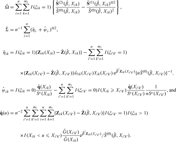The · in the subscripts indicates summing over all the subjects represented by that index. These results can be used to construct confidence intervals and to conduct hypothesis tests about β ₀.

To predict the cumulative incidence at a time t for a patient with covariates Z ₀ for right-censored data, we estimate the cumulative hazard Λ₁(t,Z ₀) = ∫λ ₁(t,Z ₀)dt by

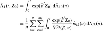where $\widehat{\beta }$ is the estimator obtained previously in this subsection. The conditional cumulative incidence estimator ${\widehat{F}}_1(t,{\mathbf{Z}}_0)=1-\text{exp}\{-{\widehat{\Lambda }}_1(t,{\mathbf{Z}}_0\left)\right\}$.

One can establish the consistency and asymptotic normality of ${\widehat{F}}_1(t,{\mathbf{Z}}_0)$ using methods similar to those in Fine and Gray (1999). The variance is rather complicated, with bootstrapping providing practicable inferences for F ₁(t,Z ₀).

4. SIMULATION STUDIES

4.1. Data generation

Numerical investigations were conducted to assess the performance of the proposed weighted estimation approach. In the following, there are 2 causes of failure. Let the subdistribution hazard for cause 1 conditionally on a frailty v _i for cluster i satisfy

(4.1)

To ensure that the cumulative incidence model unconditionally on v _i also satisfies proportional subdistribution hazard, we take v _i's to be a random sample from a positive stable distribution with parameter α. The relationship between models (2.1) and (4.1) is: λ ₁₀(t) = α M ₀ ^{(α − 1)}(t)μ ₁₀(t), where M ₀(t) = ∫₀ ^t μ ₁₀(u)du and β ₁ = α τ ₁. In the sequel, we let μ ₁₀(t) = ρ e ^{− ρt},ρ > 0 such that M ₀(∞) = 1.

Let F ₁(t;Z _ik,v _i)≡P(T _ik ≤ t,ε_ik = 1|Z _ik,v _i). By the Laplace transformation (Hougaard, 1986), (Logan and others, 2011),

An exponential distribution for P(T _ik|ε_ik = 2,Z _ik,h _i) is assumed with subdistribution hazard function h _iexp(τ ₂ ^′ Z _ik), where h _i is generated from a positive stable distribution (γ) for each i. Thus, P(T _ik|ε_ik = 2,Z _ik) is exponential with hazard γ t ^{γ − 1} exp(β ₂ ^′ Z _ik), where β ₂ = γ τ ₂. Each of β ₁,β ₂,τ ₁,τ ₂ is a p×1 vector.

Two designs are considered: cluster constant covariates design and matched design. In all cases, the model involves a scalar covariate, that is, p = 1. For each setup, data were generated repeatedly 5000 times, with the following algorithm:

• (i) Cluster sizes m _i are prespecified or randomly generated;

• (ii) For cluster constant design, covariates Z _1i1 are randomly generated from a standard normal distribution for i = 1,…,n, with Z _1ik = Z _1i1 for all k; for matched design, we let Z _1ik = 0 and Z _1ik^′ = 1, where k and k ^′ are odd and even numbers, respectively;

• (iii) v _i are randomly generated from a positive stable distribution (α), where α∈(0,1);

• (iv) h _i are randomly generated from a positive stable distribution (γ), where γ∈(0,1);

• (v) 2 − ε_ik are generated given v _i from a binary distribution with probability equaling F ₁(∞|Z _1ik,v _i) = 1 − exp( − v _i e ^τ₁Z_1ik);

• (vi) T _ik are generated from the conditional distribution of T _ik given ε_ik using inverse probability transformation.

4.2. Simulation results

We present simulation results for both cluster constant covariates design and matched design to demonstrate the performance of the clustered weighted (CW) score function relative to the clustered censoring complete (CCC) estimators and the estimators from the Fine–Gray model (described in section 3 of Fine and Gray, 1999).

For the cluster constant design, we conducted 2 batches of simulations to examine the sizes of Wald tests based on the different estimators of β ₁. In the first batch, cluster sizes are randomly generated with replacement from {2,3,4,5}; in the second batch, the cluster sizes equaled 20 for all clusters. For each batch, we first generated data by assuming the true parameter values (β ₁,β ₂) to be (0,1) with independent standard normal covariates. The parameters for within-cluster correlations (α,γ) were assumed to be (0.3,0.3),(0.3,0.7),(0.7,0.3), or (0.7,0.7), and ρ = 1. Censoring times were independently generated from a uniform [0.3,1.5] distribution to achieve 20–30% of censored observations at various levels of (α,γ).

Table 1 gives the empirical sizes of CC, CCC, weighted score (W) tests, and CW score tests for n = 100 and 250 and nominal level 0.05. Under all settings, the empirical sizes of tests not accounting for clustering (CC and W) deviate substantially from the nominal level. The CW tests and the CCC tests attain the nominal level when the number of clusters is reasonably large (250). When the number of clusters is smaller (100), their sizes are slightly larger than the nominal level.

Table 1.

Empirical sizes of tests from CC, CCC, W, and CW estimating equations with cluster-constant standard normal covariates. Cluster sizes m ∈ {2, 3, 4, 5} or 20. F ₁(t;Z _ik) = 1 – exp { – (1 – e^–t)^α  e^β′₁Z_ik}. Significance level = 0.05

α	γ	Censoring	Number of clusters	m	CC	CCC	W	CW
0.3	0.3	0.21	100	≤ 5	0.284	0.050	0.286	0.050
			250		0.275	0.056	0.276	0.056
0.3	0.7	0.22	100		0.284	0.050	0.286	0.050
			250		0.275	0.056	0.275	0.056
0.7	0.3	0.29	100		0.162	0.058	0.164	0.060
			250		0.176	0.056	0.171	0.055
0.7	0.7	0.30	100		0.162	0.058	0.165	0.060
			250		0.176	0.056	0.171	0.056
0.3	0.3	0.21	100	20	0.550	0.065	0.556	0.065
			250		0.549	0.056	0.552	0.055
0.3	0.7	0.22	100		0.550	0.065	0.557	0.065
			250		0.549	0.056	0.553	0.056
0.7	0.3	0.29	100		0.396	0.065	0.398	0.065
			250		0.396	0.053	0.397	0.052
0.7	0.7	0.30	100		0.413	0.058	0.416	0.057
			250		0.404	0.052	0.403	0.051

Next, β ₁ was set to 0.5 keeping all other parameters unchanged to assess the Wald tests under the alternative. The number of clusters is 100, with additional simulations performed with 250 and 500 clusters when (α,γ) = (0.3,0.3) to assess the impact of sample size, for which the results using other settings are similar and are omitted.

Table 2 gives $E({\widehat{\beta }}_1)$, estimated with the average of the ${\widehat{\beta }}_1$ from the 1000 replicates; $s({\widehat{\beta }}_1)$, estimated with the square root of the empirical variance of ${\widehat{\beta }}_1$; and $E(\widehat{s})$, the average of the model-based standard errors (SEs) of ${\widehat{\beta }}_1$. The 2 clustered approaches (CCC, CW) have better performance than the unclustered approaches (CC, W), in terms of the empirical coverage of the 95% confidence intervals, and the closeness of model-based variance and empirical variances, under all settings. Note that when the within-cluster correlation is larger (α = 0.3), the parameter estimate has slightly larger bias and the confidence intervals using the robust variance estimator have slightly reduced coverage versus when the correlation is smaller (α = 0.7), all other things being the same. Larger numbers of clusters, 250 and 500, lead to estimators with smaller bias and corresponding empirical coverages which achieve the nominal level.

Table 2.

Parameter estimates from CC, CCC, W, and CW estimating equations with cluster-constant standard normal covariates. Cluster sizes m ∈ {2, 3, 4, 5}. F ₁(t;Z _ik) = 1 − exp{ − (1 − e ^{− t})^αe^β′₁Z_ik}

α	γ	Censoring	Number of clusters	β1	Equation	${\widehat{\beta }}_1$	$s\left({\widehat{\beta }}_1\right)$	$E\left({\widehat{s}}_1\right)$	Coverage
0.3	0.3	0.22	100	0.5	CC	0.514	0.140	0.076	0.717
					CCC	0.514	0.140	0.134	0.938
					W	0.514	0.140	0.076	0.713
					CW	0.514	0.140	0.134	0.938
			250	0.5	CC	0.505	0.086	0.047	0.727
					CCC	0.505	0.086	0.085	0.944
					W	0.505	0.086	0.047	0.722
					CW	0.505	0.086	0.085	0.944
			500	0.5	CC	0.502	0.061	0.033	0.719
					CCC	0.502	0.061	0.060	0.948
					W	0.502	0.061	0.033	0.717
					CW	0.502	0.061	0.060	0.948
0.3	0.7	0.25	100	0.5	CC	0.514	0.140	0.076	0.717
					CCC	0.514	0.140	0.134	0.938
					W	0.514	0.140	0.076	0.712
					CW	0.514	0.140	0.134	0.938
0.7	0.3	0.30	100	0.5	CC	0.508	0.116	0.081	0.834
					CCC	0.508	0.116	0.112	0.938
					W	0.508	0.116	0.080	0.829
					CW	0.508	0.116	0.112	0.939
0.7	0.7	0.32	100	0.5	CC	0.508	0.116	0.081	0.834
					CCC	0.508	0.116	0.112	0.938
					W	0.508	0.116	0.080	0.829
					CW	0.508	0.116	0.112	0.939

For the matched design, cluster sizes were 2 and the true parameter values for β ₁ were 0, 0.12, 0.24, 0.36, 0.48, or 0.60, and assuming β ₂ to be 1. We took (α,γ,ρ) = (0.3,0.6,0.5)and (0.6,0.6,2). Censoring times were independently generated from a uniform [a,b] distribution with a and b giving censoring of 0%, 30%, and 50%.

Figure 1 depicts the powers of CC, CCC, and CW score tests at the nominal level of 0.05. Under all censoring percentages and both correlation levels, the unclustered tests have lower power than the clustered approach since the unclustered tests overestimate the variance of the parameter estimate (the corresponding model-based variance estimates are much bigger than the empirical estimates). The figure also suggests that the powers of CW tests and the CCC tests are almost the same, which is an indication of the validity of our weighting technique in the clustered case. Simulations with larger cluster sizes (m _i = 10, i.e. 5 in each arm) are also performed under the above settings, with similar results obtained.

Fig. 1.

The empirical powers of the tests for matched design.

It is worth highlighting that the simulation results are insensitive to the clustering parameter for the competing event (γ) under all settings.

5. APPLICATION

The Acute Myeloid Leukemia (AML) data arise from an ongoing bone marrow transplant registry of the European Blood and Marrow Transplant (EBMT) Group. In this analysis, the event of interest was the time from graft to the first occurrence of either acute GvHD grade 2 or chronic GvHD. Death and relapse without GvHD are the competing causes of failure. Katsahian and others (2006) proposed a frailty model for the subdistribution hazard in order to test the prognostic factors while treating the centers as clusters. A subset of the data was used with the extraction date being January 1, 2002 consisting of patients with the following inclusion criteria: (1) received either genoidentical or matched unrelated donor (MUD) stem cell transplant; (2) were more than 16 years old at the time of transplant; (3) had acute myeloid leukemia in first complete remission; (4) received a transplant between January 1, 1994 and December 31, 2004; and (5) did not receive a reduced intensity regimen nor a T-cell–depleted transplant. Centers with only one patient enroled were excluded. A total of 1022 patients from 121 clusters were included in their analysis using a frailty model.

In our analysis, we used the same registry, but with data extracted up to July 2008, while keeping other inclusion criteria from Katsahian and others (2006). The median follow-up was 1250 days, comprising patients still alive without relapse and disease. We have a total of 2952 patients from 244 centers, with 1385 GvHD and 629 competing causes of failure observed. The median number of patients per center was 6.

Since the patient populations are remarkably different across centers (Katsahian and others, 2006), there might be unobserved factors that are shared by patients within centers, potentially invalidating the use of inferences, which assume independence within centers. To address such clustering, model (2.1) is considered, where the covariates are the same as those in Katsahian and others (2006). These covariates, which are major predictive prognostic factors of GvHD, are defined as follows: Z _ik = (Z _1ik,Z _2ik,Z _3ik,Z _4ik) for the kth subject in the ith center, where i = 1,…,244,k = 1,…,m _i,and m _i∈{2,…,92}. Here, Z _1ik = I(female donor to male recipient [FM]), Z _2ik = I(source of stem cells is peripheral blood), Z _3ik = I(French-American-British [FAB] classification of AML is M5, M6, or M7), and Z _4ik = I(type of transplant is MUD). I(A) = 1 if A is true and 0 otherwise. We first fit univariable models (2.1), followed by a multivariable analysis.

The results of the coefficient estimates along with the SEs from the clustered model (robust) and the unclustered model (naive) are reported in Table 3. In the univariable and multivariable analyses, both the Fine–Gray model and the proposed marginal model indicate gender matching between donor and recipient (female donor to male recipient vs. others) is a significant prognostic factor in the subdistribution hazard of GvHD occurrence at 0.01 significance level. FAB classification of AML is significant at 0.1 level under clustered multivariable analysis but insignificant under all 3 other models. Despite the similar results for the clustered and unclustered approaches, the naive and robust variance estimators are quite different for some factors, suggesting that patients are correlated within cluster.

Table 3.

Parameter estimates in models for acute GvHD or chronic GvHD occurrence

	Univariate			Multivariable
	$\widehat{\beta }$	SE (naive)	SE (robust)	$\widehat{\beta }$	SE (naive)	SE (robust)
Female to male versus others	0.363	0.060†	0.065†	0.368	0.063†	0.068†
PBSC versus BMT	– 0.051	0.054	0.075	– 0.060	0.057	0.076
FAB M5, M6, M7 versus others	0.089	0.067	0.058	0.099	0.069	0.060‡
MUD versus genoidentical	0.049	0.081	0.103	0.086	0.087	0.108

^†Significant at 0.01 level.

^‡Significant at 0.1 level.

The estimated cumulative incidence function for 4 hypothetical patients are plotted in Figure 2. Here, we consider the source of the stem cells to be the peripheral blood, and that the transplant is from an unrelated donor. We further employed all possible combinations of the 2 significant covariates: FM and FAB classification of AML being M5, M6, or M7 (FAB1). One sees clearly that FM has a greater impact on the cumulative incidence of GvHD than does FAB classification, as evidenced by its impact on the absolute probabilities of GvHD.

Fig. 2.

The estimated cumulative incidence function.

6. DISCUSSION

The use of marginal models has been widely adopted for ordinary right-censored data. The proposed methods provide an adaptation of the Fine–Gray model for the cumulative incidence function, which rigorously accommodates both correlated failure times and correlated censoring times. Such methods are particularly useful in applications with small groups of correlated observations where the correlation is primarily a nuisance, as in multicenter trials. Frailty models are less attractive in such settings, owing to the need to explicitly model such correlations, which complicates the analysis of covariate effects.

The simulations demonstrate the potential bias and loss of power in hypothesis testing, which may arise from ignoring within-cluster correlations in variance estimation. Additional improvements in power might be achieved via more careful consideration of the correlation structure. For example, model-based approaches, like frailty models (Katsahian and others, 2006), might potentially yield such gains, at the risk of bias under model misspecification. The development of tests which yield increased power while still being robust to misspecification is a topic of future research.

An R function, CRRC, which implements the marginal analysis, is included in the supplementary material available at Biostatistics online and has been incorporated in crrSC, an R package which is publicly available on the Comprehensive R Archive Network (CRAN) site.

SUPPLEMENTARY MATERIAL

Supplementary material is available at http://biostatistics.oxfordjournals.org.

FUNDING

National Institutes of Health (NIH)/National Cancer Institute (NCI) (1R01 CA94893-02 to J.F.).

References

- Cai JW, Prentice RL. Regression estimation using multivariate failure time data and a common baseline hazard function model. Lifetime Data Analysis. 1997;3:197–213. doi: 10.1023/a:1009613313677. [DOI] [PubMed] [Google Scholar]
- Chen BE, Kramer JL, Greene MH, Rosenberg PS. Competing risks analysis of correlated failure time data. Biometrics. 2008;64:172–179. doi: 10.1111/j.1541-0420.2007.00868.x. [DOI] [PMC free article] [PubMed] [Google Scholar]
- Clayton D, Cuzick J. Multivariate generalizations of the proportional hazards model. Journal of the Royal Statistical Society. Series A (General) 1985;148:82–117. [Google Scholar]
- Fine JP, Gray RJ. A proportional hazards model for the subdistribution of a competing risk. Journal of the American Statistical Association. 1999;94:496–509. [Google Scholar]
- Gray RJ. A class of K–sample tests for comparing the cumulative incidence of a competing risk. Annals of Statistics. 1988;16:1141–1154. [Google Scholar]
- Hougaard P. Survival models for heterogeneous populations derived from stable distributions. Biometrika. 1986;73:387–396. [Google Scholar]
- Katsahian S, Resche-Rigon M, Chevret S, Porcher R. Analysing multicenter competing risks data with a mixed proportional hazards model for the subdistribution. Statistics in Medicine. 2006;25:4267–4278. doi: 10.1002/sim.2684. [DOI] [PubMed] [Google Scholar]
- Lee EW, Wei LJ, Amato DA. Cox-type regression analysis for large numbers of small groups of correlated failure time observations. In: Klein IP, Goel PK, editors. Survival Analysis: State of the Art. Dordrecht: Kluwer Academic Publishers; 1992. pp. 237–247. [Google Scholar]
- Liang KY, Self SG, Chang YC. Modelling marginal hazards in multivariate failure time data. Journal of the Royal Statistical Society. Series B, Statistical Methodology. 1993;55:441–453. [Google Scholar]
- Logan BR, Zhang MJ, Klein JP. Marginal models for clustered time to event data with competing risks using pseudovalues. Biometrics. 2011;67:1–7. doi: 10.1111/j.1541-0420.2010.01416.x. [DOI] [PMC free article] [PubMed] [Google Scholar]
- Prentice RL, Kalbfleisch JD, Peterson AV, Jr., Flournoy N, Farewell VT, Breslow NE. The analysis of failure times in the presence of competing risks. Biometrics. 1978;34:541–554. [PubMed] [Google Scholar]
- Robins JM, Rotnitzky A. Recovery of information and adjustment for dependent censoring using surrogate markers. In: Jewell N, Dietz K, Farewell V, editors. AIDS Epidemiology—Methodological Issues. Boston, MA: Birkhäuser; 1992. pp. 297–331. (includes errata sheet) [Google Scholar]
- Ruan P, Gray RJ. Analyses of cumulative incidence via parametric multiple imputation. Statistics in Medicine. 2008;27:5709–5724. doi: 10.1002/sim.3402. [DOI] [PubMed] [Google Scholar]
- Spiekerman CF, Lin DY. Marginal regression models for multivariate failure time data. Journal of the American Statistical Association. 1998;93:1164–1199. [Google Scholar]
- Wei LJ, Lin DY, Weissfeld L. Regression analysis of multivariate incomplete failure time data by modeling marginal distributions. Journal of the American Statistical Association. 1989;84:1065–1073. [Google Scholar]
- Ying Z, Wei LJ. The Kaplan–Meier estimate for dependent failure time observations. Journal of Multivariate Analysis. 1994;50:17–29. [Google Scholar]
Associated Data
This section collects any data citations, data availability statements, or supplementary materials included in this article.