IDEAL CURRENT PATTERNS YIELDING OPTIMAL SNR AND SAR IN MAGNETIC RESONANCE IMAGING: COMPUTATIONAL METHODS AND PHYSICAL INSIGHTS

Abstract

At high and ultra-high magnetic field strengths, understanding interactions between tissues and the electromagnetic fields generated by radiofrequency (RF) coils becomes crucial for safe and effective coil design, as well as for insight into limits of performance. In this work we present a rigorous electrodynamic modeling framework, using dyadic Green’s functions, to derive the electromagnetic field in homogeneous spherical and cylindrical samples resulting from arbitrary surface currents in the presence or absence of a surrounding RF shield. We show how to calculate ideal current patterns which result in the highest possible signal to noise ratio (“ultimate intrinsic signal to noise ratio (SNR)”) or the lowest possible RF power deposition (“ultimate intrinsic specific absorption rate (SAR)”) compatible with electrodynamic principles. We identify familiar coil designs within optimal current patterns at low to moderate field strength, thereby establishing and explaining graphically the near-optimality of traditional surface and volume quadrature designs. We also document the emergence of less familiar patterns, e.g. involving substantial electric as well as magnetic dipole contributions, at high field strength. Performance comparisons with particular coil array configurations demonstrate that optimal performance may be approached with finite arrays if ideal current patterns are used as a guide for coil design.

INTRODUCTION

Accurate modeling of electromagnetic (EM) effects is becoming increasingly important as higher magnetic field strengths are employed in magnetic resonance (MR) systems. The interactions of the EM field with biological tissues at high frequencies result in tissue-specific perturbations of EM field patterns, requiring appropriate coil designs to improve image quality and to avoid adverse effects in patients. Parallel MR imaging (MRI) (1–3) and parallel MR transmission (4,5) techniques are promising solutions to address these issues. In reception, the increased signal-to-noise ratio (SNR) available at higher field strengths allows for higher degrees of acceleration in parallel MRI, therefore enabling efficient imaging with reduced energy deposition and also limiting susceptibility artifacts and other time-dependent signal perturbations. In transmission, arrays of independently driven transmit coils allow for time-varying control over the EM field which can be used to improve excitation homogeneity and to minimize specific absorption rate (SAR). As the number of channels available in MR systems has increased to enable faster acquisitions and multiple coil excitations, building prototypes of coil arrays has become more difficult and expensive; therefore, the design of coil arrays has relied ever more upon electrodynamic simulations.

Numerical simulations with techniques such as the finite difference time domain (FDTD) technique are normally used for EM analyses with detailed heterogeneous models of the human body (6–8). Although these approaches are rigorous and the results have shown good agreement with experimental data, they are time-consuming and their numerical complexity grows rapidly as the number of modeled coils increases. The duration of these simulations also restricts the number of different coil-sample configurations that can be realistically explored, limiting the generality of the results. In fact, it has been shown that there is a strong dependency of SNR and SAR upon geometrical and physical factors (9–11), such as shape and dimensions of the object and the conductors, or electrical properties of the tissues. There is therefore a valuable role for rapid but rigorous electrodynamic simulation approaches that may yield insight into these fundamental dependencies using comparatively simple geometrical models.

In this work we use mode expansions with dyadic Green’s functions (DGF) (12) to characterize the full-wave EM field in a dielectric sphere. A similar DGF approach for SNR calculation was described by Vesselle et al. (13,14) and by Schnell et al. (15) in the case of a cylindrical sample, but to our knowledge such an approach has not been explored for spherical geometries until now. (Other authors have used different multipole expansions to calculate ultimate intrinsic SNR in spherical geometries (9) or to explore the SNR behavior of simple loop coils in the vicinity of spherical samples (16–18).) We also extend the cylindrical model in Ref. (15) to include the effects of the conductive shield of the MR system. Such an extension was originally summarized by Schnell in his doctoral thesis (19), a rich body of work which is currently available only in the original German. Here, we lay out the necessary extension in sufficient detail to enable straightforward numerical computations. Semi-analytical calculations of SNR and SAR for simulated MR experiments, both for specific coil geometries and for the ultimate intrinsic case, can be performed quickly with our DGF formulation. The theoretical framework also enables derivation of ideal surface current patterns corresponding to the best possible performance. We show that ideal current patterns provide useful physical insights that confirm the efficacy of traditional RF coil designs at low field strength and establish the need for new designs at high field strength. Preliminary results of this work were presented at the 2008 and 2011 meetings of the International Society for Magnetic Resonance in Medicine, in Toronto and Montreal, respectively (20–22).

THEORY

In this section, an electrodynamic formulation is presented to calculate surface current patterns associated with optimal coil performance in MR experiments with uniform samples. In the case of a spherical object, a full theoretical derivation is provided, whereas in the case of a cylindrical object an extension to the theory presented in Ref. (15) is outlined.

Electromagnetic field expansion in a dielectric sphere with dyadic Green’s functions

The DGF formalism enables calculation of the electric field resulting from any spatial current distribution J(r) as:

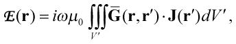[1]

where i is the imaginary unit, ω is the angular frequency, μ_o is the magnetic permeability in free space and Ḡ(r, r′) is the branch of the DGF corresponding to the region indicated by r. The DGF associated with a dielectric sphere may be constructed using the method of scattering superposition (12,21), in terms of a double series of vector wave functions in spherical coordinates:

$$\begin{array}{l}{\mathbf{M}}_{l,m}(\mathbf{r},k)=j_l(kr){\mathbf{X}}_{l,m}(\theta ,\varphi )\\ {\mathbf{N}}_{l,m}(\mathbf{r},k)=(1/k)\nabla \times {\mathbf{M}}_{l,m}(\mathbf{r},k),\end{array}$$ [2]

where l, m are the expansion indices, k is the complex wave number, X_l,m is a vector spherical harmonic of order (l, m), j_l is a spherical Bessel function of order l and spherical coordinates r (radial), θ (polar) and ϕ(azimuthal) were used. An expression for the DGF Ḡ(r, r′) used in this work and a derivation of some of the key equations to follow is provided in Appendix A.

Let us now constrain the current to flow only on a spherical surface of radius b (which need not coincide with the surface of the dielectric sphere itself):

$$\mathbf{J}(r,\theta ,\varphi )=\mathbf{K}(\theta ,\varphi )\frac{\delta (r-b)}{b^{2}sin\theta }.$$ [3]

In the most general case, the surface current density K may consist of both magnetic-type (divergence-free) and electric-type (curl-free) components, indicated with the superscript ^(M) and ^(E) respectively, and we can express it with a mode expansion. The generic surface current mode then takes the form of:

$${\mathbf{K}}_{l,m}(\theta ,\varphi )=-i\sqrt{l(l+1)}\left[W_{l,m}^{(M)}{\mathbf{X}}_{l,m}(\theta ,\varphi )+W_{l,m}^{(E)}\widehat{\mathbf{r}}\times {\mathbf{X}}_{l,m}(\theta ,\varphi )\right],$$ [4]

where $W_{l,m}^{(M)}$ and $W_{l,m}^{(E)}$ are the series expansion coefficients representing divergence-free and curl-free surface current contributions, respectively. The DGF method allows solution of the scattering problem to determine the EM field impressed upon the sphere by the vector source current density K. From Eq. [1] we derive (see Appendix A) an expression for the electric field inside the sphere and then, using Maxwell’s equations, we calculate the corresponding expression for the magnetic field:

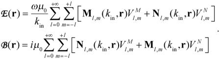[5]

Note that harmonic time variation is assumed in everything to follow, and a common factor of e^−iωt is omitted but assumed for all fields and currents throughout the theoretical derivation. The complex wave number inside the sphere is calculated as $k_{\text{in}}^2={\omega }^2{\epsilon }_r{\epsilon }_0{\mu }_0+i\omega {\mu }_0\sigma$, where ω is the angular frequency, ε_r and σ are the relative permittivity and the electrical conductivity of the dielectric material, respectively; μ_o and ε₀ are the magnetic permeability and the electric permittivity in free-space, respectively. The weighting coefficients $V_{l,m}^M$ and $V_{l,m}^N$ are derived by multiplying the expansion coefficients of the current density with a transformation matrix T that accounts for boundary conditions at the surface of the sphere:

$$\mathbf{V}=\left(\begin{array}{c}{V}_{l,m}^M\\ V_{l,m}^N\end{array}\right)=\left(\begin{array}{cc}-i\sqrt{l(l+1)}{h}_l^{(1)}(k_{0}b)C_l& 0\\ 0& {\frac{-i\sqrt{l(l+1)}}{k_{0}b}\frac{\partial [{rh}_l^{(1)}(k_{0}r)]}{\partial r}|}_{r=b}{D}_l\end{array}\right)·\left(\begin{array}{c}{W}_{l,m}^{(M)}\\ W_{l,m}^{(E)}\end{array}\right)={\mathbf{T}}^{\text{T}}·\mathbf{W},$$ [6]

where the superscript ^T indicates the transpose of the matrix, $h_l^{(1)}$ is the spherical Hankel function of the first kind of order l and the complex wave number outside the sphere is calculated as $k_0^2={\omega }^2{\mu }_0{\epsilon }_0$. The coefficients C_l and D_l in the matrix T are determined by applying the Dirichlet boundary conditions at the surface of the sphere. Note that the vectors V, T and W are defined for given (l, m).

It should be noted that the fundamental field modes M and N in Eq. [2] bear a simple relation to basis fields used in multipole expansions for the sphere (9,23), whereas the specific allowed combinations compatible with boundary conditions as specified in Eq.’s [5] and [6] may be shown to be related to other field solutions explored in the literature (17,24). In any case, the individual EM field modes in Eq. [5], matched to their associated surface current modes, can be employed as if they correspond to hypothetical coil current distributions. We may therefore find optimal weighting coefficients that allow combinations of modes for maximum SNR, or minimum SAR. Ideal current patterns are computed in each case as a weighted sum of the current modes in Eq. [4], using the same coefficients.

Calculation of ideal current patterns for ultimate intrinsic SNR

Previous studies (9,15,25,26) have shown how to derive an expression for intrinsic SNR using the magnetic field to calculate signal sensitivity functions and the electric field to calculate thermal noise due to the presence of the sample. Ultimate intrinsic SNR (UISNR) (9,15,25,26), the theoretical best possible SNR independent of any particular coil geometry, can be calculated employing the EM modes in the basis set to maximize the general SNR expression. In the case of Cartesian SENSE parallel imaging reconstructions (2), the combination of modes that results in the highest possible SNR is found by solving a constrained minimization problem which yields the following solution for the optimal series expansion coefficients (2):

$${\mathbf{W}}^{\mathit{opt}}={\left({\mathbf{S}}^H{\mathbf{\Psi }}_{\text{mode}}^{-1}\mathbf{S}\right)}^{-1}{\mathbf{S}}^H{\mathbf{\Psi }}_{\text{mode}}^{-1}$$ [7]

where S is the sensitivity matrix (2), and Ψ_mode is the modes’ noise covariance matrix. The sensitivity matrix contains the complex signal sensitivities associated with each mode at the target position r₀ and at all aliased positions:

$$\mathbf{S}(\mathbf{r})=\left(\begin{array}{ccc}{S}_1({\mathbf{r}}_0)& \dots & S_1({\mathbf{r}}_{R-1})\\ \dots & \dots & \dots \\ S_{L_{\text{mode}}}({\mathbf{r}}_0)& \dots & S_{L_{\text{mode}}}({\mathbf{r}}_{R-1})\end{array}\right),$$ [8]

where R is the acceleration (or reduction) factor and L_mode = 2(l_max+1)² is the total number of modes corresponding to the expansion order l_max, which is chosen to ensure convergence of the UISNR calculations. The elements of S can be derived by applying the principle of reciprocity (27), which allows calculation of the receive sensitivity of a coil in terms of the left circularly polarized component of the RF magnetic field that would be transmitted at the same position by a unit current flowing around the coil:

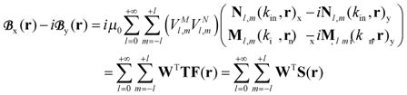[9]

The only type of noise contributing to ultimate intrinsic SNR is, by definition, sample noise, which means that any conductor is assumed to be perfect (i.e. to have zero resistance and zero reactance) and that the modes’ noise covariance matrix Ψ_mode in Eq. [7] can be calculated by simply integrating electric field products over the volume of the sphere:

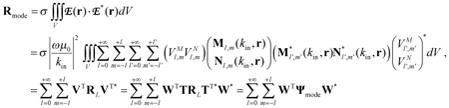[10]

where:

$${\mathbf{R}}_L=\left(\begin{array}{cc}\underset{0}{\overset{a}{\int }}{|j_l(k_{\text{in}}r)|}^2{r}^{2}dr& 0\\ 0& \frac{1}{{\left|k_{\text{in}}\right|}^2}\left\{\underset{0}{\overset{a}{\int }}\left[{\left|\frac{\partial [r{j}_l(k_{\text{in}}r)]}{\partial r}\right|}^2+l(l+1){|j_l(k_{\text{in}}r)|}^2\right]dr\right\}\end{array}\right)$$ [11]

and a and σ are the radius and the electrical conductivity of the sphere, respectively. Using the weights in Eq. [7] we can calculate the UISNR received at any particular position r₀ inside the sphere as (9):

$$\stackrel{\sim }{\zeta }({\mathbf{r}}_0)\propto \frac{{\omega }_0{M}_0{\displaystyle \sum _{l=0}^{+\infty }}{\displaystyle \sum _{m=-l}^{+l}}{\left({\mathbf{W}}^{\mathit{opt}}\right)}^{\text{T}}\mathbf{S}(\mathbf{r})}{\sqrt{4k_{\text{B}}{T}_{\text{S}}{\displaystyle \sum _{l=0}^{+\infty }}{\displaystyle \sum _{m=-l}^{+l}}{\left({\left({\mathbf{W}}^{\mathit{opt}}\right)}^{\text{T}}{\mathbf{\Psi }}_{\text{mode}}{\left({\mathbf{W}}^{\mathit{opt}}\right)}^{\ast }\right)}_{0,0}}}=\frac{{\omega }_0{M}_0}{\sqrt{4k_{\text{B}}{T}_{\text{S}}·{\left(\mathbf{S}{(\mathbf{r})}^H{\mathbf{\Psi }}_{\text{mode}}^{-1}\mathbf{S}(\mathbf{r})\right)}_{0,0}^{-1}}}$$ [12]

where M₀ is the equilibrium magnetization, ω₀ is the Larmor frequency, k_B is Boltzmann’s constant, and T_S is the absolute temperature of the sample. The “0,0” subscript in the denominator indicates the diagonal element of the matrix in parentheses with an index associated with the target position r₀.

Ideal surface current patterns associated with the ultimate intrinsic SNR are found by applying the optimal weights in Eq. [7] to the individual current modes in Eq. [4] and adding them up:

$${\mathbf{I}}_{\text{Rx}}^{\mathit{ideal}}(\theta ,\varphi )=\sum _{l=0}^{+\infty }\sum _{m=-l}^{+l}{\mathbf{K}}_{l,m}^{\mathit{opt}}(\theta ,\varphi )=-i\sum _{l=0}^{+\infty }\sum _{m=-l}^{+l}\sqrt{l(l+1)}{({\mathbf{W}}^{\mathit{opt}})}^{\text{T}}\left(\begin{array}{c}{\mathbf{X}}_{l,m}(\theta ,\varphi )\\ \widehat{\mathbf{r}}\times {\mathbf{X}}_{l,m}(\theta ,\varphi )\end{array}\right).$$ [13]

The subscript _Rx indicates that the currents refer to the signal reception case. Note that calculation of ideal current patterns is possible with the DGF formalism, but not with EM field-based mode expansions, included those used in previous works to compute UISNR for a spherical sample (9,25,26).

Calculation of ideal current patterns for ultimate intrinsic SAR

The DGF formulation extends naturally to SAR analysis in the transmit case, as the electric field resulting from the surface current distribution can be applied directly to calculate the average RF power deposition in the object (5,11). In a previous study it was shown that tailored RF excitations from multiple coils can be applied in parallel to achieve a target flip angle distribution, while simultaneously minimizing global SAR (5). Implementing such an optimization with the EM modes derived from the basis set, and using them as hypothetical transmit fields, enables calculation of ultimate intrinsic SAR (UISAR), the smallest possible global SAR (11), which depends on the desired excitation profile, but is independent of any particular coil design. In the case of an EPI excitation trajectory, assuming that time-variant quantities are sampled only at time points corresponding to positions lying on the excitation trajectory, voxel positions can be mapped by Fourier transformation to excitation k-space positions and UISAR can be expressed as (11):

$$\stackrel{\sim }{\xi }=\frac{1}{N}\sum _{n=1}^N\left[{\mathit{\mu }}_n^H{({\mathbf{C}}_n{\mathrm{\Phi }}^{-1}{\mathbf{C}}_n^H)}^{-1}{\mathit{\mu }}_n\right].$$ [14]

where N is the total number of voxels (defined as the number of time points in excitation k-space), μ_n is the target excitation at voxel n and Φ is an electric field covariance matrix, defined for each mode and equal by reciprocity to the noise covariance matrix Ψ_mode in Eq. [10]. C_n is a spatial weighting map made up of the transmit sensitivities at the voxel (or voxels, for accelerated parallel excitations) of interest and it is analogous to the matrix S in Eq. [9], with the elements transposed and the right circularly polarized component of the magnetic field, i.e. (r)+ i (r), used instead of the left circularly polarized one. Note that the theory of UISAR can be generalized in a straightforward manner to arbitrary excitation trajectories.

Ideal surface current patterns corresponding to the theoretically smallest global SAR in the transmit case can be derived by adding up the optimally weighted contributions of each current mode. In fully parallel transmission, tailored excitations are applied to individual elements, so ideal currents are calculated as a function of time, while traversing excitation k-space:

[15]

In this expression, the subscript _Tx stands for transmission, pΔt is the p-th time interval of the EPI excitation and the weights of the linear combination are found by Fourier transforming the elements of ${\mathbf{f}}_n^{\mathit{opt}}$, the optimal RF excitation patterns generated by the transmit elements (5,11):

$${\mathbf{f}}_n^{\mathit{opt}}={\mathbf{\Phi }}^{-1}{\mathbf{C}}_n^H{({\mathbf{C}}_n{\mathbf{\Phi }}^{-1}{\mathbf{C}}_n^H)}^{-1}{\mathit{\mu }}_n.$$ [16]

In RF shimming (17,28), a special time-independent case of parallel transmission where there is a single driving RF current that is delivered with distinct time-invariant phase and amplitude to each coil element, the corresponding ideal current patterns can be found following a similar SAR minimization approach (11):

$${\mathbf{I}}_{\text{Tx}}^{\mathit{ideal}}(\theta ,\varphi )=\sum _{l=0}^{+\infty }\sum _{m=-l}^{+l}{\mathbf{K}}_{l,m}^{\mathit{opt}}(\theta ,\varphi )=-i\sum _{l=0}^{+\infty }\sum _{m=-l}^{+l}\sqrt{l(l+1)}{({\alpha }^{\mathit{opt}})}^{\text{T}}\left(\begin{array}{c}{\mathbf{X}}_{l,m}(\theta ,\varphi )\\ \widehat{\mathbf{r}}\times {\mathbf{X}}_{l,m}(\theta ,\varphi )\end{array}\right).$$ [17]

In this case ideal current patterns are not modulated in time and there is a single set of optimal weighting coefficients, α^opt, for the entire excitation, which are calculated as (11):

$${\alpha }^{\mathit{opt}}={\mathbf{\Phi }}^{-1}{\mathbf{C}}_{\mathit{FOV}}^H{({\mathbf{C}}_{\mathit{FOV}}{\mathbf{\Phi }}^{-1}{\mathbf{C}}_{\mathit{FOV}}^H)}^{-1}\frac{{\mathit{\mu }}_{\mathit{FOV}}}{{\mathbf{h}}_{\mathit{FOV}}},$$ [18]

where C_FOV is a L_mode × N matrix made up of the transmit sensitivities of all modes at every voxel location, which would be identical to the matrix C_n in Eq. [16] for the case of an acceleration factor equal to the total number of voxels. h_FOV is the common RF excitation pattern that is proportional to the Fourier transform of the shared driving RF current waveform, combined with the common applied field gradients (11). Although it is shared by all transmit elements, h_FOV is modulated by the transmit field patterns of the individual coils. Note that with RF shimming the optimization is performed simultaneously for all voxels in the field of view (FOV), as it is not possible to control the EM field as a function of time.

Optimal currents for circular surface coils

After deriving the ultimate intrinsic limits, we now describe a method for comparing them against particular coil array performance. In the previous sections, we showed that we could use a complete set of basis functions to simulate the optimal SNR and SAR theoretically achievable with any possible combination of coils. The performance of any actual coil can be simulated with the same formalism by applying the appropriate weighting functions to the general current distribution in Eq. [4]. Note that this is possible because the DGF formalism solves the scattering problem rigorously, accounting for boundary conditions associated with the object geometry and its relation to the coil currents. Indeed, for circular surface coils we validate our results against the classic results of Keltner et al (16).

Let us consider a loop coil of radius R positioned outside the dielectric sphere, with its axis along the z-axis and at a distance d from the center of the sphere (Figure 1). The surface current distribution for this coil can be defined as:

$${\mathbf{K}}_z^{\mathit{coil}}(\theta ,\varphi )=\widehat{\varphi }I\frac{sin\theta }{\sqrt{d^2+R^2}}\delta \left(r-\sqrt{d^2+R^2}\right)\delta \left(cos\theta -\frac{d}{\sqrt{d^2+R^2}}\right),$$ [19]

where I is the current circulating in the coil and $\delta \left(r-\sqrt{d^2+R^2}\right)=1$, as the current is defined only on the spherical surface of radius $b=\sqrt{d^2+R^2}$. The proportionality factor $sin\theta /\sqrt{d^2+R^2}$ guarantees that the flux of ${\mathbf{K}}_z^{\mathit{coil}}$ through any half plane of constant θ (polar angle) is equal to I. The use of delta functions in Eq. [19] amounts to modeling surface current patterns as infinitely thin conductor wires. However, in the practical implementation of our DGF computations we use a finite number of basis functions (enough to ensure convergence), resulting in circulating surface current patterns and corresponding effective coil conductors with a finite width that depends on the expansion order. The known bunching of current towards the edges of flat conductive ribbons may be simulated using a sufficiently large number of modes, but we found this computationally expensive measure not to be necessary for the derivation of key physical insights, since field distributions converge relatively rapidly with mode number, and since the remaining effects of current distribution within conductor cross-sections generally result in a simple scaling of effective conductor resistivity. For simplicity, Eq. 19 also assumes a uniform distribution of current azimuthally around the coil loop – an assumption which admittedly does not hold rigorously for sufficiently long conductor paths and at sufficiently high frequency that charge separation becomes significant. Once again, this limitation is not a fundamental impediment to the generation of basic physical insights into coil and field behavior (16,17); and, as is the case for cross-sectional current distribution, if the true azimuthal current distribution is known a priori, it may certainly be simulated with our DGF formalism, using appropriate current weights.

Fig. 1.

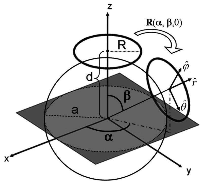
Schematic representation of the spherical sample geometry, with two exemplary loop coils arranged on a spherical surface at distance $\sqrt{d^2+R^2}$ from the center of the sphere. SNR and SAR calculations were performed on a transverse plane through the center of the object.

We can also express the coil current distribution in Eq. [19] as a weighted combination of the basis functions in Eq. [4], where the curl-free component is set to zero, as currents can only flow in closed patterns for the case of a loop coil:

$$\mathbf{K}(\theta ,\varphi )=\sum _{l=0}^{+\infty }\sum _{m=-l}^{+l}{W}_{l,m}^{(M)}\left(-i\sqrt{l(l+1)}{\mathbf{X}}_{l,m}(\theta ,\varphi )\right).$$ [20]

Eqs. [19] and [20] must be equivalent and, by comparing them, we can find an expression for $W_{l,m}^{(M)}$ associated with the particular loop coil:

$$W_{l,0}^{\mathit{coil},(M)}=\frac{-2\pi R}{(l+1)}{\left(cot\theta {\text{Y}}_l^0(\theta ,\varphi )-csc\theta \sqrt{\frac{2l+1}{2l-1}}{\text{Y}}_{l-1}^0(\theta ,\varphi )\right)}_{\theta =arccos\frac{d}{\sqrt{d^2+R^2}}}.$$ [21]

We have substituted I=1, as, for the purposes of modeling coil sensitivities by reciprocity, we are interested in unit current. The current density for a loop coil rotated to an arbitrary position on the sphere (Figure 1) has the same functional form as that of the loop coil along the z-axis, but in a coordinate system rotated with respect to the reference coordinate system:

$${\mathbf{K}}_{\mathit{rot}}^{\mathit{coil}}(\theta ,\varphi )\equiv {\mathbf{K}}_{z^{\prime }}^{\mathit{coil}}({\theta }^{\prime },{\varphi }^{\prime })=\sum _{l=0}^{+\infty }{\left(W_{l,0}^{\mathit{coil},(M)}\right)}_{\mathit{rot}}\left[-i\sqrt{l(l+1)}{\mathbf{X}}_{l,0}^{\prime }({\theta }^{\prime },{\varphi }^{\prime })\right],$$ [22]

where the weights ${\left(W_{l,0}^{\mathit{coil},(M)}\right)}_{\mathit{rot}}$ are obtained from Eq. [21] by substituting ϕ′,θ′ for ϕ,θ. Rotated vector spherical harmonics can be always represented as a linear superposition of unrotated vector spherical harmonics (29):

$${\mathbf{X}}_{l,0}^{\prime }({\theta }^{\prime },{\varphi }^{\prime })=\sqrt{\frac{4\pi }{2l+1}}\sum _{m=-l}^l{Y}_l^{m^{\ast }}(\beta ,\alpha ){\mathbf{X}}_{l,m}(\theta ,\varphi ),$$ [23]

where α and β define the angular position of the center of the rotated coil on the sphere (Figure 1). Substituting in Eq. [22], we obtain an expression for the current density of a rotated loop coil in the reference coordinate system:

$$\begin{array}{l}{\mathbf{K}}_{\mathit{rot}}^{\mathit{coil}}(\theta ,\varphi )=\sum _{l=0}^{+\infty }\sum _{m=-l}^l{\left(W_{l,0}^{\mathit{coil},(M)}\right)}_{\mathit{rot}}\sqrt{\frac{4\pi }{2l+1}}{Y}_l^{m^{\ast }}(\beta ,\alpha )\left[-i\sqrt{l(l+1)}{\mathbf{X}}_{l,m}(\theta ,\varphi )\right]\\ =\sum _{l=0}^{+\infty }\sum _{m=-l}^l{W}_{l,m}^{\mathit{coil},(M)}\left[-i\sqrt{l(l+1)}{\mathbf{X}}_{l,m}(\theta ,\varphi )\right],\end{array}$$ [24]

The optimal SNR (or SAR) for an array of L_coil receive (or transmit) loop coils can be coil calculated with Eq. [12] (or Eq. [14]), after applying the weights $W_{l,m}^{\mathit{coil},(M)}$ to the receive (or transmit) sensitivity of each loop coil and to the elements of the noise resistance matrix:

[25]

where c is the coil index, ranging from 1 to L_coil. In the transmit case Ψ̃_mode = Ψ_mode = Φ, as RF power deposition is calculated with the volume integral in Eq. [10]. In the receive case, Ψ̃_mode should include all sources of noise affecting SNR. In this work, in addition to the intrinsic noise due to the sample (see Eq. [10]), we modeled coil noise, which is the second largest noise contribution and can be calculated in a straightforward manner with the DGF formalism. Thus, for SNR calculations Ψ̃_mode = Ψ_mode + R_A = TR_LT^T* + R_A, where R_L is defined in Eq. [11] and the additional term, R_A, which accounts for resistive power losses in the coil conductors, can be calculated by integrating the current distribution on the spherical surface A′ with radius b, where the coil lies:

$$\begin{array}{l}{\stackrel{\sim }{\text{R}}}_A=\frac{1}{{\sigma }_c{d}_c}\underset{A^{\prime }}{\iint }\mathbf{K}({\mathbf{r}}^{\prime })·{\mathbf{K}}^{\ast }({\mathbf{r}}^{\prime }){dA}^{\prime }\\ =\frac{1}{{\sigma }_c{d}_c}\underset{A^{\prime }}{\iint }\sum _{l=0}^{+\infty }\sum _{m=-l}^{+l}\sum _{l^{\prime }=0}^{+\infty }\sum _{m^{\prime }=-l^{\prime }}^{+l^{\prime }}\left(W_{l,m}^{\mathit{coil},(M)}0\right)\left(\begin{array}{c}{\mathbf{K}}_{l,m}^{(M)}\\ 0\end{array}\right)\left({\mathbf{K}}_{l^{\prime },m^{\prime }}^{\ast (M)}0\right){\left(\begin{array}{c}{W}_{l^{\prime },m^{\prime }}^{\mathit{coil},(M)}\\ 0\end{array}\right)}^{\ast }{dA}^{\prime }\\ =\sum _{l=0}^{+\infty }\sum _{m=-l}^{+l}\left(W_{l,m}^{\mathit{coil},(M)}0\right)\frac{l(l+1)b^2}{{\sigma }_c{d}_c}\left(\begin{array}{cc}1& 0\\ 0& 1\end{array}\right){\left(\begin{array}{c}{W}_{l^{\prime },m^{\prime }}^{\mathit{coil},(M)}\\ 0\end{array}\right)}^{\ast }=\sum _{l=0}^{+\infty }\sum _{m=-l}^{+l}\left(W_{l,m}^{\mathit{coil},(M)}0\right){\mathbf{R}}_A{\left(\begin{array}{c}{W}_{l^{\prime },m^{\prime }}^{\mathit{coil},(M)}\\ 0\end{array}\right)}^{\ast }.\end{array}$$ [26]

We see that the current flowing in the conductors causes a power loss inversely proportional to the electrical conductivity (σ_c) and thickness ( d_c) of the coil material. In calculating UISNR, we assume perfect conductors with infinite conductivity and therefore R_A becomes zero. It is important to note that Johnson noise is only one aspect of the resistance of loop coils and it is considered here to explore general dependencies. However, for the purpose of actual coil design optimization, it is possible to integrate a realistic coil noise model that includes radiation loss, substrate material loss, and losses associated with lumped circuit elements, solder joints, etc. (30).

Electromagnetic field expansion in a dielectric cylinder surrounded by a conductive shield

In order to compute ideal current patterns also in the case of a cylindrical sample, we used the EM field expansion described by Schnell et al. (15) and we extended it, following a general prescription in (19), to include the conductive shield of the MR scanner in the model. This general model has three distance scales of interest, representing three concentric cylindrical layers: the radius a of the dielectric cylinder, the radius ρ_c of the cylindrical surface where the current distribution of putative transmit or receive coils is defined, and the radius ρ_s of the encircling conductive shield. The generic current mode on the surface of the current-bearing cylinder at radius ρ_c takes the form of:

$${\mathbf{K}}_n(m,\varphi ,z)=W_n^{(M)}(m)\nabla \times e^{in\varphi }{e}^{\mathit{imz}}\widehat{\rho }+W_n^{(E)}(m)\nabla e^{in\varphi }{e}^{\mathit{imz}}$$ [27]

and the vector wave functions used to construct the DGF are:

$$\begin{array}{l}{\mathbf{M}}_{n,q}(m,\mathbf{r})=\nabla \times J_n(q\rho )e^{in\varphi }{e}^{\mathit{imz}}\widehat{z}\\ {\mathbf{N}}_{n,q}(m,\mathbf{r})=\frac{1}{k_{\text{in}}}\nabla \times \nabla \times J_n(q\rho )e^{in\varphi }{e}^{\mathit{imz}}\widehat{z}\end{array}$$ [28]

where n, m are the expansion indices, J_n(qρ) is a Bessel function of integer order n and the eigenvalue parameter q is defined either as $q=\gamma =\sqrt{k_{\text{in}}^2-m^2}$, with k_in as in Eq. [5], or $q=\eta =\sqrt{{k_0}^2-m^2}=\sqrt{{\omega }^2{\epsilon }_0{\mu }_0-m^2}$, for the region inside and outside the cylinder, respectively. The expression for the EM field inside the dielectric cylinder can be calculated similarly, yielding the same general expression as in Ref. (15):

[29]

For this work, we re-derived the transformation matrix T that multiplies the currents weights (see Eq. [6]), to account for boundary conditions due to the MR conductive shield surrounding the cylinder:

$${\mathbf{T}}^{\text{T}}=-j\frac{4{\pi }^2{\rho }_c}{{\eta }^2}\left\{\begin{array}{l}\left(H_n^{{(2)}^{\prime }}(\eta {\rho }_c)-\frac{H_n^{{(2)}^{\prime }}(\eta ,{\rho }_s)}{J_n^{\prime }(\eta ,{\rho }_s)}{J}_n^{\prime }(\eta {\rho }_c)\right)\left[\begin{array}{c}{e}_n(m)\\ f_n(m)\end{array}\right]\left[\begin{array}{cc}\eta m& \eta n/{\rho }_c\end{array}\right]\\ +\left(H_n^{(2)}(\eta {\rho }_c)-\frac{H_n^{(2)}(\eta ,{\rho }_s)}{J_n(\eta ,{\rho }_s)}{J}_n(\eta {\rho }_c)\right)\left[\begin{array}{c}{g}_n(m)\\ h_n(m)\end{array}\right]\left[\begin{array}{cc}{nk}_0/{\rho }_c& (m/k_0)\left({(n/{\rho }_c)}^2-{\eta }^2\right)\end{array}\right]\end{array}\right\}$$ [30]

Here $H_n^{(2)}(\eta ,{\rho }_s)$ is the Hankel function of the second kind of order n evaluated at the shield radius ρ_s, and the coefficients e, f, g, and h contain all the relevant information from the boundary conditions requiring field continuity at the cylinder surface (see Ref. (15)).

Note that the EM field derived with our DGF formalism (Eq. [29]) can be described in terms of TE and TM modes as in classical EM wave theory. Explicitly calculating the cross products in Eq. [28] yields the following expressions for wave functions in the interior of the dielectric cylinder:

$$\begin{array}{l}{\mathbf{M}}_{n,\gamma }(m,\mathbf{r})=\nabla \times J_n(\gamma \rho )e^{in\varphi }{e}^{\mathit{imz}}\widehat{z}=\left(i\frac{n}{\rho }{J}_n(\gamma \rho )\widehat{\rho }-\gamma J_n^{\prime }(\gamma \rho )\widehat{\varphi }\right)e^{in\varphi }{e}^{\mathit{imz}}\\ {\mathbf{N}}_{n,\gamma }(m,\mathbf{r})=\frac{1}{k_{\text{in}}}\nabla \times {\mathbf{M}}_{n,\gamma }(m,\mathbf{r})=\left(i\frac{\gamma m}{k_{\text{in}}}{J}_n^{\prime }(\gamma \rho )\widehat{\rho }-\frac{nm}{k_{\text{in}}\rho }{J}_n(\gamma \rho )\widehat{\varphi }+\frac{{\gamma }^2}{k_{\text{in}}}{J}_n(\gamma \rho )\widehat{z}\right)e^{in\varphi }{e}^{\mathit{imz}}\end{array}$$ [31]

A simplified case in which the shield radius is set equal to the radius of the dielectric cylinder may be recognized as the familiar configuration of a uniform dielectric-filled cylindrical waveguide. In this case, the encircling shield forces a null in tangential electric field at the shield radius, which selects for particular modes with zeros of either $J_n^{\prime }(\gamma b)$ (which sets the tangential component of M to zero) or J_n(γb) (which sets the tangential component of N to zero). Since the Bessel function and its derivative never have coincident zeros, only one or the other is allowed as the electric field, i.e. either $V_n^M(m)$ or $V_n^N(m)$ vanishes. If ∞ M_n,γ(m,r), we have a TE mode, since M has no z component. In this TE case, ∞ N_n,γ(m,r) and the magnetic field does have a z component. Alternatively, we can have ∞ N_n,γ(m,r) and ∞ M_n,γ(m,r), which is a TM mode. Our broader formulation with distinct object radius, coil radius, and shield radius represents a generalization to a partially-filled waveguide driven by currents on an intermediate cylindrical surface. Any arbitrary allowed field may then be understood as a superposition of generalized waveguide modes.

Optimal currents for cylindrical window coils

The general formalism and Eqs [25] and [26] can be applied to calculate optimal SNR and SAR for cylindrical window coils surrounding a dielectric cylinder (see Fig. 1 in Ref. (14)). Current density distribution for an ideal cylindrical window coil centered at ϕ= 0 and z= 0 with angular aperture 2ϕ₀ and axial length 2d carrying current I on each leg is:

$${\mathbf{K}}^{\mathit{window}}(\varphi ,z)=I\left\{\begin{array}{l}(\delta (z+d)-\delta (z-d))(\theta (\varphi -{\varphi }_0)-\theta (\varphi +{\varphi }_0))\widehat{\varphi }+\frac{1}{{\rho }_c}(\delta (\varphi -{\varphi }_0)-\delta (\varphi +{\varphi }_0))(\theta (z-d)-\theta (z+d))\widehat{z}\end{array}\right\}$$ [32]

Here θ (ϕ−ϕ₀) is the step function with a positive step from 0 to 1 at ϕ=ϕ₀. Note also that we have used the notation ρ_c instead of b for the coil radius, in distinction to Vesselle et al (14) whose derivations we have used to validate our results regarding cylindrical window coils. The factor of 1/ρ_c in the z component arises from the requirement of uniform current around the loop:

$$\int {\mathbf{J}}^{\text{window}}·(\rho d\varphi d\rho \widehat{z})={\rho }_c\int {\mathbf{K}}^{\text{window}}·\widehat{z}d\varphi =I=\int {\mathbf{K}}^{\text{window}}·\widehat{\varphi }dz=\int {\mathbf{J}}^{\text{window}}·(\mathit{dzd}\rho \widehat{\varphi }).$$ [33]

(Similar caveats to those elaborated earlier for the circular loop coil apply in this case regarding the use of ideal delta functions and step functions in Eq. [32] and the corresponding assumption of filamentary wires carrying uniform current.) Using the Fourier transformation properties of the delta function and the step function, we have:

$$\begin{array}{l}{\mathbf{K}}^{\text{window}}(\varphi ,z)=I\sum _{n=-\infty }^{\infty }\underset{-\infty }{\overset{\infty }{\int }}\left\{\begin{array}{l}\frac{sin(n{\varphi }_0)}{n}{e}^{in\varphi }\left(e^{\mathit{imd}}-e^{\mathit{imd}}\right)e^{\mathit{imz}}\widehat{\varphi }+\frac{1}{{\rho }_c}\left(e^{-in{\varphi }_0}-e^{in{\varphi }_0}\right)e^{in\varphi }\frac{sin(md)}{m}{e}^{\mathit{imz}}\widehat{z}\end{array}\right\}dm\\ =\sum _{n=-\infty }^{\infty }\underset{-\infty }{\overset{\infty }{\int }}\left(2I\frac{sin(n{\varphi }_0)}{n}\frac{sin(md)}{m}\right)e^{in\varphi }{e}^{\mathit{imz}}\left\{im\widehat{\varphi }-\frac{in}{{\rho }_c}\widehat{z}\right\}dm\end{array}$$ [34]

This expression must be equivalent to the magnetic-dipole component of the current distribution in Eq. 27 for ρ=ρ_c:

$$\mathbf{K}(\varphi ,z)=\sum _{n=-\infty }^{+\infty }\underset{-\infty }{\overset{+\infty }{\int }}{W}_n^{(M)}(m)\nabla \times e^{in\varphi }{e}^{\mathit{imz}}\widehat{\rho }dm=\sum _{n=-\infty }^{+\infty }\underset{-\infty }{\overset{+\infty }{\int }}{W}_n^{(M)}(m)\left\{im\widehat{\varphi }-\frac{in}{{\rho }_c}\widehat{z}\right\}{e}^{in\varphi }{e}^{\mathit{imz}}dm$$ [35]

Comparing the last two equations we find an expression for the weighting coefficients:

$$W_n^{\mathit{window},(M)}(m)=2I\frac{sin(n{\varphi }_0)}{n}\frac{sin(md)}{m}$$ [36]

The effects of translation or rotation of the coil on the cylindrical surface (i.e. moving the coil center to ϕ=Δϕ_l and z=Δz_l, where l is the coil index) may be accounted for by taking ϕ→ ϕ− Δ ϕ_l and z→z − Δz_l in the preceding derivation, resulting in the following general expression for the current mode weights of a cylindrical window coil arbitrarily positioned on the cylindrical surface:

$$W_{n,l}^{\mathit{window},(M)}(m)=2\frac{sin(n{\varphi }_{0_l})}{n}\frac{sin({md}_l)}{m}{e}^{-in\mathrm{\Delta }{\varphi }_l}{e}^{-im\mathrm{\Delta }{z}_l}$$ [37]

METHODS

SNR and SAR calculations were performed on a transverse plane (Figure 1) through the center of a sphere with uniform electrical properties, chosen to approximate average values in the human head (Table 1) as in Ref. (9). SAR was calculated assuming a 3D EPI pulse, optimized to provide a homogeneous excitation profile over the two-dimensional FOV. We used sphere radius a of 10 cm and the current distribution was defined on a spherical surface concentric with the object having radius b equal to 10.5 cm. Finite arrays of identical loop coils, with different number of elements and various geometrical arrangements on the spherical surface of radius b, were modeled in this work. Annealed copper conductivity (58×10⁶ S·m⁻¹) and conductor thickness equal to skin depth at the operating frequency associated with each field strength was assumed. Calculations were implemented in Matlab (MathWorks, Natick, MA, USA) using an expansion order l_max = 70, to ensure convergence. For the case of a cylindrical object, we modeled a uniform cylinder with 20 cm radius and assumed dielectric properties of dog skeletal muscle (Table 1) as in Ref. (15). The current distribution and the conductive shield were defined at a distance ρ_c = 20.5 cm and ρ_s = 34.25 cm from the axis of the cylinder, respectively. The expansion coefficients m and n were varied from −50 to +50, and from −40 to +40, respectively, to ensure convergence. The coefficient n was varied with unit step, whereas m, which in theory should be continuous, was varied with step Δm = 1/L, where L = 40 cm was chosen to represent the typical extension of the FOV in the z direction. For the purposes of validation and in order to document the generality of our DGF method, tailored expansion coefficients and geometrical parameters were also used to replicate the results of various previous studies not specifically addressed at ideal current patterns.

RESULTS

Comparison with previous studies

Figure 2 shows that simulation results reported elsewhere in the literature for the cases of spherical and cylindrical samples can be replicated precisely using our DGF formalism. Figure 2a plots DGF results, which reproduce a portion of Figure 5 in Ref. (9) (originally computed using a multipole field expansion), showing the behavior of UISNR as a function of position along the radius of a 30 cm diameter dielectric sphere, for different values of the main magnetic field strength. The DGF-derived curves in Figure 2b reproduce those of Figure 2 in Ref. (16) (also based on a multipole expansion), illustrating the SNR behavior of a loop coil placed above a dielectric sphere as a function of frequency. (Note that, in order to achieve a good match with Ref. (16), it was necessary to use a reduced number of modes with l_max = 23 in our DGF calculations. This number is smaller than we generally found to be required for full convergence at high frequencies.) Figure 2c replicates part of Figure 7 in Ref. (15), which plots the UISNR as a function of field strength for a cylindrical object surrounded by a current surface carrying magnetic dipole only vs. magnetic plus electric dipole current components. DGF results in Figure 2d reproduce one of the two plots in Figure 5 from Ref. (14), showing the SNR of a cylindrical window coil as a function of coil offset for different locations inside a dielectric cylinder. The four sets of plots in Figure 2 are nearly identical replicas of previously published data, validating the accuracy and indicating the flexibility of our DGF calculations.

Fig. 2.

Representative results from previous studies replicated, for the sake of validation, using the current DGF formalism. a) DGF results matching Figure 5 in Ref. (9): UISNR as a function of radial position in the transverse plane of a 30 cm diameter dielectric sphere for varying B₀. b) DGF results matching Figure 2 in Ref. (16): SNR as a function of frequency for a 12 cm diameter loop coil, its axis aligned with the B₀ field direction, suspended 2 cm above a 20 cm diameter dielectric sphere. Values are calculated for a voxel 5 cm beneath the surface of the sphere (on axis) and normalized to the SNR at 430 MHz. c) DGF results matching Figure 7 in Ref. (15): UISNR on the axis of a 20 cm radius dielectric cylinder as a function of frequency is compared for an optimal lossless cylindrical current surface built of magnetic dipoles only and a similar optimal current surface built of both magnetic and electric dipoles. d) DGF results matching Figure 5 in Ref. (14): SNR of a cylindrical window coil as a function of coil position at 40 MHz in a 20 cm radius dielectric cylinder. Each plot corresponds to a different position of the voxel of interest along the radial dimension of the cylinder.

Fig. 5.

Ideal surface current patterns associated with the best possible SNR for a voxel position intermediate between the center and the surface of the sphere at 1.5 T. On the left-hand side of the top row, current patterns are plotted for an arbitrary time point on a two-dimensional “unwrapped” view of the spherical surface, whereas on the right-hand side, a schematic representation shows how the current patterns evolve in time. In the middle and bottom rows, three-dimensional representations and explanatory diagrams of the current patterns are shown for four time points, respectively. Ideal currents patterns are localized near the voxel of interest and alternate between distributed single-loop and distributed figure-eight, or butterfly, configurations every Δωt = π/2, inverting direction every Δωt = π.

SNR efficiency

Ultimate intrinsic SNR and optimal SNR for finite coil arrays were calculated within the same theoretical framework, allowing for direct comparison, without concern about differential scaling factors. Figure 3 shows SNR efficiency, with respect to the best possible performance, of arrays of loop coils symmetrically packed around the spherical sample, at different voxel locations and for different values of the main magnetic field strength. Neglecting noise contributions due to coil conductors, the SNR of both arrays near the center of the object converges rapidly to the ultimate value at low field, whereas the relative performance of the array with fewer elements worsens at higher frequencies. For a voxel near the surface of the sphere (r = 0.95a), where the ultimate SNR assumes its highest values, array performance is considerably lower and even with 64 coils the resulting SNR is less than 15% of the optimum at all field strengths tested. If we include coil-derived power losses, the SNR of both arrays decreases, although the 8-element array is less affected by the additional noise contribution.

Fig. 3.

SNR as a function of main magnetic field strength, at different distances from the center of the spherical sample. Ultimate intrinsic SNR is compared to the SNR of finite arrays of loop coils, with 8 and 64 elements, uniformly distributed around the spherical object. The case in which only sample-derived noise contributions are considered is shown separately from the case in which both sample-derived and coil-derived noise contributions are considered. Adding coil-derived noise in the model reduces SNR, especially at high field. For each plot, data are normalized to the highest value.

Ideal current patterns

Since current patterns are time-varying complex valued quantities, in order to see how they truly behave, we multiplied the current modes by the time-varying factor e^−iωt, which had been removed from the equations presented earlier for simplicity, and took the real part. In the case of a voxel at the center of a sphere, displaying ideal current patterns associated with the best possible SNR as a function of time results in two large distributed current loops, centered on the x–y plane (θ = 90°) and separated by 180 degrees in the azimuthal direction, which rotate in the same sense about an axis that precesses around the direction (z-axis) of the main magnetic field (Figure 4). On the top of Figure 4, a snapshot of the ideal current patterns is visualized on a 2D “unwrapped” view of the spherical surface where the current distribution is defined. Next to the 2D view, a schematic drawing illustrates the essential time evolution. On the bottom of the figure, 3D views of the ideal current patterns are shown together with schematic representations of the rotations, for four time points separated from each other by a quarter of a cycle. In the perfectly symmetric case of a voxel at the center of the sphere, the shape of the ideal current patterns was the same at all simulated field strengths. This rotating current configuration represents an ideal volume quadrature arrangement, in which a field constant in amplitude and rotating with the spins at the Larmor frequency is created at the center of the sphere.

Fig. 4.

Ideal surface current patterns associated with the best possible SNR at a voxel in the center of the sphere. On the left-hand side of the top row, current patterns are plotted for an arbitrary time point on a two-dimensional “unwrapped” view of the spherical surface, whereas on the right-hand side, a schematic representation shows how the current patterns evolve in time (via the harmonic time dependence e^−iωt). In the middle and bottom rows, three-dimensional representations and explanatory diagrams of the current patterns are shown for four time points, respectively. For all simulated field strengths (1.5 T to 11 T), ideal currents patterns for a voxel in the center take the form of two distributed loops on opposite sides of the sphere, which rotate in the same sense about an axis that precesses around the z-axis.

Figure 5 shows ideal current patterns at 1.5 T for a voxel at an intermediate position (r = 5 cm, θ = 90°, ϕ= 45°) between the center and the surface of the sphere. In this case, the currents flow only in the proximity of the voxel of interest, alternating between distributed single-loop and distributed figure-eight, or butterfly, configurations every quarter of a cycle, and inverting direction every half cycle. This current distribution enables the net field experienced by the spins at the target voxel position to precess with the spins around the z direction at the Larmor frequency. However, ideal current patterns deviate from such familiar quadrature detection behavior and become more complex at higher field strength (see Figure 6).

Fig. 6.

Ideal surface current patterns associated with the best possible SNR for a voxel position intermediate between the center and the surface of the sphere at 11 T. In the top row, current patterns are plotted for an arbitrary time point on a two-dimensional “unwrapped” view of the spherical surface. In the bottom row, three-dimensional representations of the current patterns are shown for four time points, respectively. Ideal currents patterns continue to show an alternating pattern, but the simple loop-butterfly configuration seen at 1.5T in Figure 4 is distorted.

Temporal snapshots of ideal current patterns for a voxel on the axis of a cylinder at 0.2 T and 7 T are shown in Figures 7 and 8, respectively. The plots represent 2D “unwrapped” views of the 3D cylindrical surface where the current distribution is defined. At 0.2 T, the currents appear to form two distributed loops separated by 180 degrees, which precess at the Larmor frequency around the axis of the cylinder. This is analogous to the spherical case in Fig 3.

Fig. 7.

Ideal surface current patterns associated with the best possible SNR at a voxel on the axis of a cylindrical sample at 0.2 T. On the left-hand side of the top row, current patterns are plotted for an arbitrary time point on a two-dimensional “unwrapped” view of the cylindrical surface (with the axial and azimuthal coordinates on the horizontal and vertical axis, respectively), whereas on the right-hand side, a schematic representation shows how the current patterns evolve in time. In the middle and bottom rows, the current patterns are shown together with explanatory diagrams for four time points. Ideal currents patterns, which resemble the rotating dual distributed-loop pattern seen in a sphere (Figure 3), may also be recognized as a distributed birdcage-like pattern, in which z-directed “rung” currents vary sinusoidally around the circumference of the cylinder, connected by encircling “end-ring” return currents. The entire current pattern precesses at the Larmor frequency around the axis of the cylinder (i.e. the z-axis).

Fig. 8.

Ideal surface current patterns associated with the best possible SNR at a voxel on the axis of a cylindrical sample at 7 T. In the top row, current patterns are plotted for an arbitrary time point on a two-dimensional “unwrapped” view of the cylindrical surface. In the bottom row, the current patterns are shown for four time points separated by Δωt = π/2. Ideal current patterns precess around the axis of the cylinder (i.e. the z-axis). Although sinusoidal variation of z-directed currents is maintained here (reflecting a dominant mode order), apparent loss of the “end-ring” currents seen at lower field strength (Figure 6) indicates an increased contribution of curl-free or electric-dipole current components at high field strengths.

Closer inspection reveals that the amplitude of current in fact varies sinusoidally with φ, completing one full cycle around the circumference of the cylinder. Near z = 0, the current is directed largely along z, whereas nearer to z = ±L/4, the current consolidates into circumferentially-directed “end-rings” patterns. In other words, the ideal current pattern for a central voxel resembles a birdcage coil (31), albeit one with smooth distributed currents and with a considerably narrower extent along z than is typically used in volume coil designs. At 7 T, the current patterns become more complex and the circumferentially-directed portions near the edges of the axial FOV, which at 0.2 T resemble end-ring return currents, seem to disappear. Note that in the plot at the top of both figures, the z axes extend to twice the dimension of the axial FOV to show that the distance between periodic repetitions of the EM field, governed by the expansion coefficient m, is sufficient to ensure that the current patterns are confined within the length of the FOV. This means that for our purposes we are effectively modeling a finite cylinder of length L, even if the electrodynamic derivation assumes that the cylinder is infinite along the axial direction (15). Ideal current patterns for a voxel at an intermediate position between the axis and the surface of the cylinder (not shown) follow alternating loop-butterfly patterns very similar to those for an intermediate voxel in the case of the sphere (see Figures 5 and 6).

The absence of end-ring return currents in Figure 8 suggests that, at 7 T frequencies, ideal currents are no longer constrained to travel in complete loops. Divergence-free and curl-free contributions of the ideal current patterns in Figures 7 and 8 are plotted separately in Figure 9 for an arbitrary time point. Figure 9 shows that the weight of the curl-free component increases at high field and affects the final shape of the current patterns. In fact, at 0.2 T, the dominant contribution is from the closed-loop (divergence-free) current component, whereas at 7 T the shape of the ideal current patterns is considerably affected by the electric-dipole (curl-free) component.

Fig. 9.

Ideal surface current patterns associated with the best possible SNR at a voxel on the axis of a cylindrical sample are compared at 0.2 T and 7 T for an arbitrary time point. The plots represent two-dimensional “unwrapped” views of the cylindrical surface. The axial and azimuthal coordinates are on the horizontal and vertical axis, respectively. Divergence-free and curl-free contributions to the ideal current patterns are plotted separately to the right of the combined pattern at each field strength. For ease of visualization, divergence-free and curl-free patterns are scaled independently to a common amplitude, but the size of the diagonal arrows indicates the relative magnitude of the contribution of each subpattern to the net current pattern at each field strength. At 0.2 T, the divergence-free magnetic dipole pattern dominates, whereas at 7 T the combined current distribution more closely resembles the curl-free electric dipole pattern.

Ideal current patterns for a voxel at the center of the sphere at 7 T are shown again in Figure 10, juxtaposed to the effective current patterns of optimally-combined finite coil arrays. The ideal currents circulate in wide loops surrounding the spherical surface and we see that with 64 coils, symmetrically arranged around the object, it is possible to capture most of this behavior, as the resulting SNR is 91% of its theoretical limit. With 8 coils, the current patterns, which are constrained by the position of the conductors, only cover a limited region of the spherical surface and the resulting performance is lower. Figure 11 shows that, for a voxel intermediate between the center and the surface, a single loop with radius equal to the distance between the center of the coil and the voxel of interest divided by the square root of five (i.e. R = 24.6 mm), which has been described to be optimal in the case of a lossy half space (32,33), yields 68% of the ultimate SNR at 1.5 T (or, as indicated in parentheses in the left column of the figure, only 46% at 7 T). Figure 11 also shows that combining three identical coils (R = 35.7 mm) to form a typical surface quadrature array (figure-eight and a loop coil) that resembles the shape of the ideal current patterns at 1.5 T, yields 94% of the optimum performance, whereas using 12 loop coils with the same dimensions of those used in the quadrature configuration, but arranged symmetrically around the x–y plane, yields 93%. On the contrary, the larger array becomes more effective at 7 T, where the current patterns have a more complex and less symmetric shape. Note that, although results are reported also for 7 T, the current patterns in Figure 11 refer to 1.5 T.

Fig. 10.

Ideal surface current patterns associated with the best possible SNR at a voxel in the center of a sphere are compared, at 7 T, with SNR-optimized current patterns for an 8-element and a 64-element array at a single time-point. The corresponding SNR, normalized to the ultimate intrinsic SNR, is reported for both coils above the current plots.

Fig. 11.

Ideal surface current patterns associated with the best possible SNR at a voxel position intermediate between the center and the surface of a sphere are compared, at 7 T, with SNR-optimized current patterns for different coil configurations. Current patterns are shown for two time points separated by Δωt = π/2. The corresponding SNR values, normalized to the ultimate intrinsic SNR, are reported in the left-hand column. The performance with respect to the ultimate intrinsic SNR of the same array configurations at 7 T is reported in parentheses. The radius of the single loop coil is equal to 24.6 mm, i.e. the distance between the coil center and the voxel of interest, divided by square root of five. The radius of the other coil configurations was chosen empirically to be 35.7 mm, in order to resemble the shape of the ideal current patterns.

In Figure 12 we show ideal current patterns in the transmit case, corresponding to the excitation of a homogeneous flip angle distribution on the transverse plane through the center of the sphere (see Figure 1), with the theoretically smallest SAR. The optimization was performed for the case of RF shimming, as this technique involves a single hard pulse in the center of k-space, resulting in a single set of current patterns with a relatively straightforward harmonic time dependence (as opposed to the case of fully parallel excitation, in which optimal current patterns vary for each location in excitation k-space, and therefore each corresponding time point). Ideal current patterns were calculated by summing the optimal contributions of each current mode. A snapshot at t = 0 s is displayed in Figure 12 for six different values of the main magnetic field strength. We note that highly complex current patterns are needed in order to compensate for B₁ inhomogeneities and minimize SAR at high field. In Figure 13, results for the 7 T case are presented in more detail, using a 2D view of the spherical surface and four snapshots separated by a quarter of a cycle. Ideal current patterns appear to wrap around the sphere in the shape of two spirals, one above and one below the equator, twisting in opposite directions.

Fig. 12.

Ideal current patterns resulting in the lowest possible SAR with RF shimming, during the excitation of a homogeneous flip-angle profile across a transverse plane through the center of the sphere. The distributed loop shapes at 1.5 T are compared with increasingly complex patterns at higher field strength.

Fig. 13.

Ideal current patterns resulting in the lowest possible SAR with RF shimming, during the excitation of a homogeneous flip-angle profile across a transverse plane through the center of the sphere at 7 T. In the top row, current patterns are plotted for an arbitrary time point on a two-dimensional “unwrapped” view of the spherical surface. In the bottom row, three-dimensional representations of the current patterns are shown for four time points, separated by a quarter of a cycle.

DISCUSSION

We have presented a theoretical formalism based on DGF to calculate ideal current patterns yielding optimal SNR and SAR within homogeneous spherical and cylindrical samples. Although ideal current patterns for MR signal reception are derivable from the formalism used by Schnell et al. (15) in their study of the unaccelerated UISNR for the case of a cylindrical object, actual ideal current patterns were presented for spherical objects and for particular cylindrical cases for the first time by the authors at a recent conference (20,21). At an earlier conference, Reykowski and Fischer had previously shown surface magnetization density maps corresponding to optimum SNR for a voxel on the axis of a cylindrical sample, and had used them as a guideline to design novel V-shaped coil structures that could increase SNR at high field strengths (34). However, surface magnetization density, which may be related to magnetic dipole current density, does not include electric dipole current elements, and the patterns they showed do not reflect the increasing contribution of electric dipole elements at high field strength. Here we have shown how ideal current patterns, including both magnetic and electric dipole elements, may be computed in practice, and have demonstrated that they provide useful insight into the physical behavior of RF fields, which can be used to optimize coil design. Our method also allows for fast simulations to calculate SNR and SAR in the ultimate intrinsic case, as well as in the case of finite coil arrays.

Our results (see Figures 4 and 7) show that at low field strength the ideal current distribution yielding the optimal SNR at the center of both spherical and cylindrical samples consists of distributed current loops, which precess around the direction of the main magnetic field at the Larmor frequency. In other words, in order to maximize SNR at the center of the object, the receive field should track as closely as possible the precession of central spins. One way of achieving this is to receive with a quadrature birdcage coil (31). Indeed, ideal current patterns in Figures 4 and 7 directly resemble a sinusoidal birdcage mode rotating at the Larmor frequency (i.e. driven in quadrature). Although birdcage coils have been used for years in the field of magnetic resonance, and previous studies have shown that they can approach the ultimate intrinsic SNR near the center of a cylinder (19,33), our DGF formalism for the first time has allowed direct graphical demonstration both of their near-optimality for deep-tissue imaging and of the nature of their deviation from ideal behavior.

On the other hand, when we are interested in imaging at locations closer to the surface of the object, our results demonstrate that surface quadrature coils are nearly optimal. In particular, the combination of a single loop with a figure-eight, or butterfly, coil, which is one of the possible surface quadrature configurations (35), reaches 94% of the theoretical optimal performance at 1.5 T, compared with 68% achieved by a single loop. Wang et al. (36) also identified a distributed surface quadrature configuration as optimal for imaging below the surface of a lossy infinite half-space, using quasi-static EM calculations, which combined a large number of small loop elements tiling the planar surface. Our full-wave DGF model demonstrates that this general configuration maintains its optimality near the surface of finite objects at low to moderate field strengths. Our DGF model also identifies perturbations to the ideal configuration as field strength increases.

The results shown in Figure 11 validate to some extent the traditional use of loop elements in receive head arrays. However, the decreased coil performance at 7 T (see values in parentheses in the left column of Figure 11) suggests that this traditional choice may not be optimal at high field strengths. In fact, Figure 9, which separates current patterns around a cylinder into divergence-free and curl-free components, documents a departure from the familiar quadrature coil behavior. At 0.2 T (left half of Figure 9), the dominant contribution (indicated by the large arrow and the top panel) is from the closed-loop (divergence-free) current component resembling a quadrature birdcage mode, whereas at 7 T (right half of Figure 9) the shape of the ideal current pattern deviates significantly towards the electric-dipole (curl-free, bottom panel) component. A TEM coil (37), which also lacks an endring current, bears some resemblance to this electric-dipole pattern on an interior surface, but the TEM coil is typically surrounded by a closely adjacent shield, whose mirror currents likely perturb the system away from strict ideality. The example of Figure 9 illustrates how unshielded electric dipole components, which are required to describe a fully-general surface current pattern (15) but which have often been dismissed as inefficient for MR based on low-field experience, can become important contributors to SNR at high field strengths.

To our knowledge, there are no prior studies in the literature presenting ideal current patterns yielding minimum SAR for RF transmission. In this work, we have demonstrated how to calculate these ideal current patterns both for the case of fully parallel transmission and for RF shimming. Since in fully parallel transmission there is a different set of ideal current patterns for each timepoint or position in excitation k-space, for simplicity we have chosen to show results only for the special case of RF shimming in which the same RF pulse envelope is played out in multiple coils with distinct but time-invariant amplitudes and phases, resulting in a net current pattern with a simple harmonic time variation.

The complexity of the current patterns in the second row of Figure 12 suggests that the curl-free component may also be critical in the transmit case, in order to achieve homogeneous excitations with the lowest possible SAR. Although traditional closed-loop conductors may not be capable of approaching the best possible performance at 7 T and above, adding electric-dipole elements to coil arrays may raise concern about patient safety, due to comparatively large electric fields close to the body surface, and the potential for high local SAR even in the presence of reduced global SAR. However, just as the question of the relative efficiency of electric dipole elements requires revisiting at high field strength, these practical safety issues may benefit from dedicated attention and design. For example, in a recent abstract presented at the 2010 meeting of the International Society for Magnetic Resonance in Medicine (38), the authors proposed a novel dipole antenna for high field MRI, reporting higher B₁₊ penetration and lower SAR compared with traditional stripline elements.

Another way to improve coil performance at high field strength is to use the ideal current patterns as a guideline to design the position and shape of the conductors. For example, Figure 6 suggests that an asymmetric quadrature receive coil may be more effective at 11 T than the more typical loop and figure-eight configuration shown in Figure 11. In fact, it has been shown (34,39,40) that transmit/receive coil designs that account for the natural asymmetry of the EM field at high frequency results in improved performance compared to other designs traditionally used at low field. The natural curling of the EM field could also explain the results in Figure 12, where the spiral shape of the ideal current patterns, with a larger number of turns as field strength increases, may indeed represent a method to generate a transmit field twisting in the opposite direction in order to create a uniform excitation profile across the FOV. Alsop et al. (41) have already shown some advantages of producing spiral current patterns for high field MRI. They proposed a spiral version of the standard birdcage resonator, which enables one to create a linear phase variation along the direction of the main magnetic field in order to improve RF field homogeneity in the transverse plane.

The focus of this paper has been the generation and interpretation of ideal current patterns. Of course, the techniques used here also provide estimates of ultimate intrinsic SNR and SAR. Apart from the results in Figure 3, however, general trends in UISNR and UISAR were not explicitly explored in this work, as these have been extensively analyzed in previous studies (9,11,15). The results shown in Figure 3 regarding the efficiency of finite arrays with respect to the best possible performance are in agreement with previous observations, based on similar coil and sample models (10,18), but derived with a different electrodynamic approach, based on a multipole expansion in the sphere (23). It should, however, be noted that there are a number of advantages in using the DGF method described in this work to calculate the SNR and SAR of surface coils. First of all, with the multipole expansion it is cumbersome to derive the weighting coefficients required to express the EM field of a surface coil in terms of the basis set of modes (16), whereas this is more intuitive to do in the DGF current-based mode expansion. Furthermore, the calculation of coil sensitivity and noise covariance matrices in the case of multiple receivers/transmitters, which requires repetitive application of rotation matrices with the multipole approach (11), is performed in the DGF formalism by applying a simple transformation to the expansion coefficients, exploiting convenient properties of vector spherical harmonics. As the mode expansion is based on current distributions, another advantage is that it is straightforward to incorporate a realistic noise model that accounts for resistive losses in the coil conductors, without the need for an additional specific formulation (10,18).

The method we have developed can serve as a useful toolkit for coil designers. It allows investigation of the dependency of SNR and SAR on a multitude of factors by means of very fast simulations. Although our formalism can be useful to investigate general trends which may be expected to hold in many cases and it has already proven to provide crucial physical insights for the design of a 7 Tesla array for carotid (40) and spine (39) imaging, there may still be variations associated with particular heterogeneous examples that are not taken into account. However, note that the general DGF method is not restricted to the use of homogenous samples, but can be extended to multi-layered samples with spherical or cylindrical symmetry, by deriving the appropriate DGF with suitable boundary conditions.

It must be noted that ultimate intrinsic SNR is calculated separately for each voxel, whereas ultimate intrinsic SAR is a global quantity that accounts for total RF power deposition for a given target excitation. The fact that ideal current patterns in the receive case vary on a voxel-by-voxel basis and in the transmit case vary depending upon the target excitation pattern suggests that a large number of coils may be required to design an array with optimized performance for different applications. One approach to design the “ultimate array” is to employ genetic algorithms (42) to search for the arrangement of the conductors that enables one to generate the largest set of ideal current patterns for a given number of receive/transmit channels. Another approach would be to simulate an array with a very large number of channels that is optimal on average for various applications, convert it into a set of modes via a combiner-network, and select the modes that contribute most to the array performance, in order to achieve a similar outcome with a practical number of channels (43). A third strategy, proposed at a recent conference (44), is to arrange the conductors in order to maximize flexibility in allowed current patterns, relying on the fact that ideal current patterns would be the natural choice when employing SAR-optimal pulse sequences, or SNR-optimal reconstruction methods.

CONCLUSION

In this work we described a semi-analytical method to calculate RF coil performance based on a mode expansion using dyadic Green’s functions in a dielectric sphere. We also extended a previously described approach for the case of a dielectric cylinder. Ultimate intrinsic SNR and SAR can be computed by employing a complete set of surface current modes, and the corresponding ideal surface current patterns can be derived. Alternatively, actual coil conductor arrangements can be expanded in terms of the same current mode basis, and the resulting SNR and SAR may be compared with ultimate intrinsic results. Ideal current patterns provide useful physical insights for the design of RF coils. Our results, for the first time, confirm and explain graphically the near-optimality of common volume and surface quadrature coil designs at low to moderate field strength. The complexity and variability of ideal current patterns at higher frequencies suggests that innovative coil designs, which might confound our low-field instincts, may be needed in order to approach the optimal performance at ultra-high field.

TABLE I.

Dielectric Properties of Average Brain Tissue (Gray Background) And Dog Skeletal Muscle Tissue (White Background)

Bo [T]	1	3	5	7	9	11
Larmor Frequency [MHz]	42.6	127.7	212.9	298.1	383.2	468.4
Dielectric Constant εr	102.5	63.1	55.3	52	50	48.8
	66.6	50.3	46.8	45.3	44.5	43.9
Conductivity σ[1/Ωm]	0.36	0.46	0.51	0.55	0.59	0.62
	0.29	0.31	0.32	0.33	0.33	0.34

APPENDIX A

Dyadic Green’s functions for a dielectric sphere in free space

The dyadic Green’s function (DGF) relates a vector point source current at position r′ to the excited electric or magnetic fields at position r. Therefore, choosing the appropriate DGF enables calculation of the EM field due to any given current distribution (see Eq. [1]). We begin by defining two spherical vector wave functions that are solutions of the vector wave equation ∇ × ∇ × F − k²F = 0:

$$\begin{array}{l}{\mathbf{M}}_{l,m}(\mathbf{r})=\nabla \times \left({\psi }_{l,m}(\mathbf{r})\mathbf{r}\right)\\ {\mathbf{N}}_{l,m}(\mathbf{r})=\frac{1}{k}\nabla \times \nabla \times \left({\psi }_{l,m}(\mathbf{r})\mathbf{r}\right)\end{array}$$ [A.1]

where k is the complex wave number and ψ_lm (r) are eigenfunctions that are solutions of the scalar wave equation ∇²ψ+ k²ψ= 0 in spherical coordinates:

$${\psi }_{l,m}(\mathbf{r})=\sqrt{\frac{2l+1}{4\pi }\frac{(l-m)!}{(l+m)!}}{j}_l(kr)P_l^m(cos\theta )e^{im\phi }=j_l(kr){\text{Y}}_l^m(\theta ,\phi ).$$ [A.2]

In this expression, $P_l^m(cos\theta )$ is the associated Legendre function of order (l, m), where l and m are both integers, j_l is a spherical Bessel function of order l, and ${\text{Y}}_l^m$ is a spherical harmonic. Substituting Eq. [A.2] in Eq. [A.1] and normalizing for simplicity by $-i\sqrt{l(l+1)}$ we obtain the expressions in Eq. [2].

For the case of a dielectric sphere of radius a immersed in free space, with its center located at the origin of the coordinate system (Figure 1), the DGF can be constructed using the method of scattering superposition (12,21):

$$\overline{\mathbf{G}}(\mathbf{r},{\mathbf{r}}^{\prime })=\{\begin{array}{ll}{\overline{\mathbf{G}}}_o(\mathbf{r},{\mathbf{r}}^{\prime })+{\overline{\mathbf{G}}}_s^{(1)}(\mathbf{r},{\mathbf{r}}^{\prime })\hfill & r\ge a\hfill \\ {\overline{\mathbf{G}}}_s^{(2)}(\mathbf{r},{\mathbf{r}}^{\prime })\hfill & r\le a\hfill \end{array}$$ [A.3]

Here the source is at location r′ and r is the position at which the field is calculated. The DGF in free space is defined as (12):

$${\overline{\mathbf{G}}}_o(\mathbf{r},{\mathbf{r}}^{\prime })={ik}_0\sum _{l=0}^{+\infty }\sum _{m=-l}^{+l}\{\begin{array}{ll}{\mathbf{M}}_{l,m}^{+}(k_0,\mathbf{r}){\mathbf{M}}_{l,m}(k_0,{\mathbf{r}}^{\prime })+{\mathbf{N}}_{l,m}^{+}(k_0,\mathbf{r}){\mathbf{N}}_{l,m}(k_0,{\mathbf{r}}^{\prime })\hfill & \mathbf{r}\ge {\mathbf{r}}^{\prime }\hfill \\ {\mathbf{M}}_{l,m}(k_0,\mathbf{r}){\mathbf{M}}_{l,m}^{+}(k_0,{\mathbf{r}}^{\prime })+{\mathbf{N}}_{l,m}(k_0,\mathbf{r}){\mathbf{N}}_{l,m}^{+}(k_0,{\mathbf{r}}^{\prime })\hfill & \mathbf{r}\le {\mathbf{r}}^{\prime }\hfill \end{array}$$ [A.4]

where k₀ is the complex wave number outside the sphere that was defined for Eq. [6] and the superscript ⁺ indicates that $h_l^{(1)}$, the spherical Hankel function of the first kind of order l, is used in place of the j_l’s in Eq. [A.2]. The scattering components of the DGF are defined as (12):

$$\begin{array}{l}{\overline{\mathbf{G}}}_s^{(1)}(\mathbf{r},{\mathbf{r}}^{\prime })={ik}_0\sum _{l=0}^{+\infty }\sum _{m=-l}^{+l}\left[A_l{\mathbf{M}}_{l,m}^{+}(k_0,\mathbf{r}){\mathbf{M}}_{l,m}^{+}(k_0,{\mathbf{r}}^{\prime })+B_l{\mathbf{N}}_{l,m}^{+}(k_0,\mathbf{r}){\mathbf{N}}_{l,m}^{+}(k_0,{\mathbf{r}}^{\prime })\right]\\ {\overline{\mathbf{G}}}_s^{(2)}(\mathbf{r},{\mathbf{r}}^{\prime })={ik}_0\sum _{l=0}^{+\infty }\sum _{m=-l}^{+l}\left[C_l{\mathbf{M}}_{l,m}(k_{\text{in}},\mathbf{r}){\mathbf{M}}_{l,m}^{+}(k_0,{\mathbf{r}}^{\prime })+D_l{\mathbf{N}}_{l,m}(k_{\text{in}},\mathbf{r}){\mathbf{N}}_{l,m}^{+}(k_0,{\mathbf{r}}^{\prime })\right]\end{array}$$ [A.5]

where k_in is the complex wave number inside the sphere that was defined for Eq. [5] and the coefficients A_l, B_l, C_l and D_l are determined applying the Dirichlet boundary conditions:

$$\begin{array}{l}\widehat{\mathbf{r}}\times \overline{\mathbf{G}}(r=a+)=\widehat{\mathbf{r}}\times \overline{\mathbf{G}}(r=a-)\\ \widehat{\mathbf{r}}\times \nabla \times \overline{\mathbf{G}}(r=a+)=\widehat{\mathbf{r}}\times \nabla \times \overline{\mathbf{G}}(r=a-)\end{array}$$ [A.6]

which yields:

$$\begin{array}{l}\left(\begin{array}{cccc}-h_l^{(1)}(k_{0}a)& 0& j_l(k_{\text{in}}a)& 0\\ 0& {-\frac{[{rh}_l^{(1)}(k_{0}r)]}{\partial r}|}_{r=a}& 0& {\frac{k_0}{k_{\text{in}}}\frac{\partial [{rj}_l(k_{\text{in}}r)]}{\partial r}|}_{r=a}\\ {-\frac{\partial [{rh}_l^{(1)}(k_{0}r)]}{\partial r}|}_{r=a}& 0& {\frac{\partial [{rj}_l(k_{\text{in}}r)]}{\partial r}|}_{r=a}& 0\\ 0& -h_l^{(1)}(k_{0}a)& 0& \frac{k_{\text{in}}}{k_0}{j}_l(k_{\text{in}}a)\end{array}\right)\left(\begin{array}{c}{A}_l\\ B_l\\ C_l\\ D_l\end{array}\right)=\left(\begin{array}{c}{j}_1(k_{0}a)\\ {\frac{\partial [{rj}_1(k_{0}r)]}{\partial r}|}_{r=a}\\ {\frac{\partial [{rj}_1(k_{0}r)]}{\partial r}|}_{r=a}\\ j_l(k_{0}a)\end{array}\right)\end{array}$$ [A.7]

Mode expansion of the electromagnetic field inside a dielectric sphere

Using a basis set of current patterns defined by Eqs. [3] and [4], in order to calculate the EM field inside the sphere, we need to choose the branch of the DGF with r ≤ a and substitute in Eq. [1]:

[A.8]

Let us define the weighting coefficients of the vector wave functions as:

$$\begin{array}{l}{V}_{(l,m),(l^{\prime },m^{\prime })}^M=C_l\underset{A^{\prime }}{\iint }[W_{l^{\prime },m^{\prime }}^{(M)}{\mathbf{M}}_{l,m}^{+}(k_0,{\mathbf{r}}^{\prime })·\left(-i\sqrt{l^{\prime }(l^{\prime }+1)}{\mathbf{X}}_{l^{\prime },m^{\prime }}({\theta }^{\prime },{\phi }^{\prime })\right)+W_{l^{\prime },m^{\prime }}^{(E)}{\mathbf{M}}_{l,m}^{+}(k_0,{\mathbf{r}}^{\prime })\widehat{\mathbf{r}}\times \left(-i\sqrt{l^{\prime }(l^{\prime }+1)}{\mathbf{X}}_{l^{\prime },m^{\prime }}({\theta }^{\prime },{\phi }^{\prime })\right)]{dA}^{\prime }\\ V_{(l,m),(l^{\prime },m^{\prime })}^N=D_l\underset{A^{\prime }}{\iint }[W_{l^{\prime },m^{\prime }}^{(M)}{\mathbf{N}}_{l,m}^{+}(k_0,{\mathbf{r}}^{\prime })·\left(-i\sqrt{l^{\prime }(l^{\prime }+1)}{\mathbf{X}}_{l^{\prime },m^{\prime }}({\theta }^{\prime },{\phi }^{\prime })\right)+W_{l^{\prime },m^{\prime }}^{(E)}{\mathbf{N}}_{l,m}^{+}(k_0,{\mathbf{r}}^{\prime })\widehat{\mathbf{r}}\times \left(-i\sqrt{l^{\prime }(l^{\prime }+1)}{\mathbf{X}}_{l^{\prime },m^{\prime }}({\theta }^{\prime },{\phi }^{\prime })\right)]{dA}^{\prime }\end{array}$$ [A.9]

Applying the orthogonality relations of the vector spherical harmonics (23) we can solve the integrals in Eq. [A.9] and derive Eq. [6]. Substituting in Eq. [A.8] and using Maxwell’s equations and the symmetrical relations of the vector wave functions (see Eq. [A.1]), we can derive Eq. [5].

References

- 1.Sodickson DK, Manning WJ. Simultaneous acquisition of spatial harmonics (SMASH): fast imaging with radiofrequency coil arrays. Magn Reson Med. 1997;38(4):591–603. doi: 10.1002/mrm.1910380414. [DOI] [PubMed] [Google Scholar]
- 2.Pruessmann KP, Weiger M, Scheidegger MB, Boesiger P. SENSE: sensitivity encoding for fast MRI. Magn Reson Med. 1999;42(5):952–962. [PubMed] [Google Scholar]
- 3.Griswold MA, Jakob PM, Heidemann RM, Nittka M, Jellus V, Wang J, Kiefer B, Haase A. Generalized autocalibrating partially parallel acquisitions (GRAPPA) Magn Reson Med. 2002;47(6):1202–1210. doi: 10.1002/mrm.10171. [DOI] [PubMed] [Google Scholar]
- 4.Katscher U, Bornert P, Leussler C, van den Brink JS. Transmit SENSE. Magn Reson Med. 2003;49(1):144–150. doi: 10.1002/mrm.10353. [DOI] [PubMed] [Google Scholar]
- 5.Zhu Y. Parallel excitation with an array of transmit coils. Magn Reson Med. 2004;51(4):775–784. doi: 10.1002/mrm.20011. [DOI] [PubMed] [Google Scholar]
- 6.Collins CM, Smith MB. Calculations of B(1) distribution, SNR, and SAR for a surface coil adjacent to an anatomically-accurate human body model. Magn Reson Med. 2001;45(4):692–699. doi: 10.1002/mrm.1092. [DOI] [PubMed] [Google Scholar]
- 7.Ibrahim TS, Mitchell C, Schmalbrock P, Lee R, Chakeres DW. Electromagnetic perspective on the operation of RF coils at 1.5–11. 7 Tesla. Magn Reson Med. 2005;54(3):683–690. doi: 10.1002/mrm.20596. [DOI] [PubMed] [Google Scholar]
- 8.Kangarlu A, Ibrahim TS, Shellock FG. Effects of coil dimensions and field polarization on RF heating inside a head phantom. Magn Reson Imaging. 2005;23(1):53–60. doi: 10.1016/j.mri.2004.11.007. [DOI] [PubMed] [Google Scholar]
- 9.Wiesinger F, Boesiger P, Pruessmann KP. Electrodynamics and ultimate SNR in parallel MR imaging. Magn Reson Med. 2004;52(2):376–390. doi: 10.1002/mrm.20183. [DOI] [PubMed] [Google Scholar]
- 10.Wiesinger F. PhD Thesis. Swiss Federal Institute of Technology; Zurich: 2005. Parallel Magnetic Resonance Imaging: Potential and Limitations at High Fields; p. 149. [Google Scholar]
- 11.Lattanzi R, Sodickson DK, Grant AK, Zhu Y. Electrodynamic constraints on homogeneity and radiofrequency power deposition in multiple coil excitations. Magn Reson Med. 2009;61(2):315–334. doi: 10.1002/mrm.21782. [DOI] [PMC free article] [PubMed] [Google Scholar]
- 12.Tai CT. Dyadic Green Functions in Electromagnetic Theory. Institute of Electrical & Electronics Engineers; 1994. p. 343. [Google Scholar]
- 13.Vesselle H, Collin RE. The Signal-to-Noise Ratio of Nuclear Magnetic Resonance Surface Coils and Application to a Lossy Dielectric Cylinder Model - Part I: Theory. IEEE Trans Biomed Eng. 1995;42(5):497–506. [Google Scholar]
- 14.Vesselle H, Collin RE. The Signal-to-Noise Ratio of Nuclear Magnetic Resonance Surface Coils and Application to a Lossy Dielectric Cylinder Model - Part II: The Case of Cylindrical Window Coils. IEEE Trans Biomed Eng. 1995;42(5):507–520. [Google Scholar]
- 15.Schnell W, Renz W, Vester M, Ermert H. Ultimate Signal-to-Noise-Ratio of Surface and Body Antennas for Magnetic Resonance Imaging. IEEE Trans Antennas Propag. 2000;48(3):418–428. [Google Scholar]
- 16.Keltner JR, Carlson JW, Roos MS, Wong ST, Wong TL, Budinger TF. Electromagnetic fields of surface coil in vivo NMR at high frequencies. Magn Reson Med. 1991;22(2):467–480. doi: 10.1002/mrm.1910220254. [DOI] [PubMed] [Google Scholar]
- 17.Hoult DI, Phil D. Sensitivity and power deposition in a high-field imaging experiment. J Magn Reson Imaging. 2000;12(1):46–67. doi: 10.1002/1522-2586(200007)12:1<46::aid-jmri6>3.0.co;2-d. [DOI] [PubMed] [Google Scholar]
- 18.Wiesinger F, De Zanche N, Pruessmann KP. Approaching ultimate SNR with finite coil arrays. Proceedings of the 13h Annual Meeting of ISMRM; 7–13 May 2005; Miami Beach. p. 672. [Google Scholar]
- 19.Schnell W. PhD Thesis. Ruhr-Universitat Bochum; 1997. Rauschoptimierung von Oberflachen- und Ganzkorperantennen fur die Kernspintomographie; p. 129. [Google Scholar]
- 20.Lattanzi R, Grant AK, Sodickson DK. Approaching ultimate SNR and ideal current patterns with finite surface coil arrays on a dielectric cylinder. Proceedings of the 16th Annual Meeting of ISMRM; 3–9 May 2008; Toronto. p. 1074. [Google Scholar]
- 21.Lattanzi R, Sodickson DK. Dyadic Green’s functions for electrodynamic calculations of ideal current patterns for optimal SNR and SAR. Proceedings of the 16th Annual Meeting of ISMRM; 3–9 May 2008; Toronto. p. 78. [Google Scholar]
- 22.Lattanzi R, Sodickson DK. Physical insights from ideal current patterns resulting in ultimate intrinsic SNR: efficacy of traditional coils designs at low field strength and the need for new designs at high field. Proceedings of the 19th Annual Meeting of ISMRM; 7–13 May 2011; Montreal. p. 3876. [Google Scholar]
- 23.Jackson JD. Classical Electrodynamics. Wiley; 1998. [Google Scholar]
- 24.Tropp J. Image brightening in samples of high dielectric constant. J Magn Reson. 2004;167(1):12–24. doi: 10.1016/j.jmr.2003.11.003. [DOI] [PubMed] [Google Scholar]
- 25.Ocali O, Atalar E. Ultimate intrinsic signal-to-noise ratio in MRI. Magn Reson Med. 1998;39(3):462–473. doi: 10.1002/mrm.1910390317. [DOI] [PubMed] [Google Scholar]
- 26.Ohliger MA, Grant AK, Sodickson DK. Ultimate intrinsic signal-to-noise ratio for parallel MRI: electromagnetic field considerations. Magn Reson Med. 2003;50(5):1018–1030. doi: 10.1002/mrm.10597. [DOI] [PubMed] [Google Scholar]
- 27.Hoult DI. The Principle of Reciprocity in Signal Strength Calculations - A Mathematical Guide. Concepts Magn Reson. 2000;12(4):173–187. [Google Scholar]
- 28.Vaughan JT, Adriany G, Snyder CJ, Tian J, Thiel T, Bolinger L, Liu H, DelaBarre L, Ugurbil K. Efficient high-frequency body coil for high-field MRI. Magn Reson Med. 2004;52(4):851–859. doi: 10.1002/mrm.20177. [DOI] [PubMed] [Google Scholar]
- 29.Rose ME. Elementary Theory of Angular Momentum. J. Wiley and Sons; 1963. [Google Scholar]
- 30.Duan Q, Sodickson DK, Zhang B, Wiggins GC. A Comprehensive Coil Resistance Composition Model for High Field. Proceedings of the 18h Annual Meeting of ISMRM; 1–7 May 2010; Stockholm. p. 3858. [Google Scholar]
- 31.Hayes CE, Edelestein WA, Schenck JF, Mueller OM, Eash M. An Efficient, Highly Homogeneous Radiofrequency Coil for Whole-Body NMR Imaging at 1.5 T. J Magn Reson. 1985;63:622–628. [Google Scholar]
- 32.Roemer PB, Edelstein WA. Ultimate sensitivity limits of surface coils. New York: 1987. p. 410. [Google Scholar]
- 33.Reykowski A. PhD Thesis. Texas A&M University; 1996. Theory and design of synthesis array coils for magnetic resonance imaging; p. 288. [Google Scholar]
- 34.Reykowski A, Fischer H. V-Cage and V-Array: Novel coil structures for higher field strengths. Proceedings of the 13h Annual Meeting of ISMRM; 7–13 May 2005; Miami Beach. p. 950. [Google Scholar]
- 35.Kumar A, Bottomley PA. Optimized quadrature surface coil designs. Magma. 2008;21(1–2):41–52. doi: 10.1007/s10334-007-0090-2. Epub 2007 Dec 2004. [DOI] [PMC free article] [PubMed] [Google Scholar]
- 36.Wang J, Reykowski A, Dickas J. Calculation of the signal-to-noise ratio for simple surface coils and arrays of coils. IEEE Trans Biomed Eng. 1995;42(9):908–917. doi: 10.1109/10.412657. [DOI] [PubMed] [Google Scholar]
- 37.Vaughan JT, Hetherington HP, Otu JO, Pan JW, Pohost GM. High frequency volume coils for clinical NMR imaging and spectroscopy. Magn Reson Med. 1994;32(2):206–218. doi: 10.1002/mrm.1910320209. [DOI] [PubMed] [Google Scholar]
- 38.Ipek O, Raaijmakers AJR, Klomp DWJ, Lagendijk JJ, Van den Berg CAT. A Novel Radiative Surface Antenna for High Field Mri. Proceedings of the 18h Annual Meeting of ISMRM; 1–7 May 2010; Stockholm. p. 3799. [Google Scholar]
- 39.Duan Q, Sodickson DK, Lattanzi R, Zhang B, Wiggins GC. Optimizing 7T Spine Array Design Through Offsetting of Transmit and Receive Elements and Quadrature Excitation. Proceedings of the 18th Annual Meeting of ISMRM; 1–7 May 2010; Stockholm. p. 51. [Google Scholar]
- 40.Wiggins GC, Zhang B, Lattanzi R, Sodickson DK. B1+ and SNR optimization of high field RF coils through offsetting of transmit and receive elements. Proceedings of the 17h Annual Meeting of ISMRM; 18–24 April 2009; Honolulu. p. 2951. [Google Scholar]
- 41.Alsop DC, Connick TJ, Mizsei G. A spiral volume coil for improved RF field homogeneity at high static magnetic field strength. Magn Reson Med. 1998;40(1):49–54. doi: 10.1002/mrm.1910400107. [DOI] [PubMed] [Google Scholar]
- 42.Mitchell M. An Introduction to Genetic Algorithms. The MIT Press; 1998. p. 221. [Google Scholar]
- 43.King SB, Varosi SM, Duensing GR. Optimum SNR data compression in hardware using an Eigencoil array. Magn Reson Med. 2010;63(5):1346–1356. doi: 10.1002/mrm.22295. [DOI] [PubMed] [Google Scholar]
- 44.Zhu Y. Constellation Coil. Proceedings of the 18h Annual Meeting of ISMRM; 1–7 May 2010; Stockholm. p. 46. [Google Scholar]