Feature identification in circadian rhythms of mice strains using in vivo information

Abstract

The objective of this work was to identify strain-specific characteristics from real-time measurements of circadian rhythms of two inbred mouse strains. In particular, heart rate, temperature, and activity data collected from A/J and C57BL/6J (B6) mice using telemetry are analyzed. The influence of activity on heart rate and temperature is minimized by correlation analysis followed by regression analysis. The correlation analysis is used to determine the length of the activity data filter that results in the best correlation between activity data and heart rate or temperature. After the activity data are filtered, they are used in regression analysis. The temperature and heart rate rhythms obtained as the intercepts of the regression analysis are interpreted as the zero-activity rhythms and consequently are good estimates of the circadian rhythms. The circadian temperature rhythms for the B6 mice follow a smoother cosine-like time waveform, whereas those for the A/J mice follow a more square-wave-like waveform. To quantify the difference between these two temperature rhythms, a feature based on Fourier analysis of the time-series data is used. Detrended fluctuation analysis is used to identify features in the heart rate rhythms. The results of this work show that the features for the circadian temperature and heart rate rhythms can be used as distinguishing characteristics of the A/J and B6 strains. This work provides the foundation for future studies directed at investigating the influence of chromosomal substitutions on the regulation of circadian rhythms in these two strains.

Introduction

An important challenge in systems biology is to characterize the dynamic manner in which many physiologic, neurologic, metabolic, and immunologic systems change. These temporal changes can be regular, such as circadian and ultradian rhythms, and stochastic, such as the responses to environmental perturbations. Occasionally, prior information is available to guide decisions about what biological properties to monitor and when these should be measured. In most cases, however, this information is not available and as a result continuous (or virtually continuous) monitoring of many attributes of these biological systems is necessary.

The temporal analysis of data from biological systems presents two general challenges. The first involves the technical aspects of data acquisition. For example, the development of devices that can continuously and simultaneously monitor various chemical, electrical, and molecular properties of the system being studied in real time. The second challenge involves analysis of these high-density data streams. Time-series analysis of such data must include distinguishing signal from noise and testing the acquired signals for temporal patterns of each data type as well as quantifying the statistical and biological variability of the various biological properties being studied.

Because each individual in a population or strain is genetically unique and functions in different ways in both health and disease, accounting for genetic variation is an essential consideration in these studies. As a result, systems biology studies must test for distinct patterns of variation among and within individual data sets. Significant and consistent phenotypic differences between inbred strains are strong evidence for genetic control, and these phenotypic differences can be used to identify the genes that control circadian rhythms and to characterize the functional basis for correlated patterns of change over time. Many traits can be studied, from transcription profiles and molecular, biochemical, and physiologic properties to features of the intact organism.

Taking these various considerations into account, we set out to monitor with telemetry several simple but key biological features, namely, heart rate, temperature, and activity, in two commonly used inbred strains of laboratory mice and then to analyze the temporal variability of these features within and between the two strains.

The identification of strain-specific heart rate and temperature time-series features that characterize the circadian rhythms for different mouse strains is an important first step in developing a deeper understanding of how chromosomal substitutions can influence these rhythms, and for determining what potential biological mechanisms may be responsible for any observed differences. The two mice strains studied in this article are A/J and C57BL/6J (B6) strains, and chromosomal substitution data for these two strains are available in the literature (Hoit et al. 2002; Nadeau et al. 2000). The genetic variation in cardiovascular traits of these strains are characterized in Hoit et al. (2002). The goal of our work was to characterize strainspecific behavior using features obtained from the circadian heart rate and temperature rhythms. Heart rate, temperature, and activity data measured using telemetry are used in the analysis. Temperature and heart rate rhythms have both endogenous and exogenous components, where the exogenous components are mainly due to activity (Weinert and Waterhouse 1998; Weinert et al. 2003). Weinert and Waterhouse (1998) review the available methods developed in the literature for eliminating the activity effect from this type of data. It is observed that these methods assume an instantaneous effect of activity on temperature. However, they also show that temperature is affected by an accumulated activity level over a period of time and use correlation analysis to find the time window that gives the best correlation between temperature and activity. They also use the same analysis for heart rate in one of their other works (Weinert et al. 2003). After filtering the data using the time window determined from a correlation analysis of the temperature and activity data, regression analysis is applied. Gradients computed from the regression analysis determine the sensitivity of temperature to activity for different times of the day, and intercepts from the regression curves are good estimates of the endogenous rhythm (Weinert and Waterhouse 1998). We also eliminate the activity effect using the correlation and regression analyses developed in Weinert and Waterhouse (1998).

Once the effect of activity is eliminated from both the heart rate and temperature signals, we define features for the resulting circadian data that can be used to identify strain differences. Fourier analysis and detrended fluctuation analysis (DFA) of the circadian time series are used to identify features for the temperature and heart rate rhythms, respectively. Using these defined features, mice belonging to the B6 or A/J strains can be quantitatively classified into distinct groups. These features will also enable quantitative classification of the temporal patterns of temperature and heart rate circadian rhythms of a consomic mouse in terms of the characteristics identified for the parental strains studied in this article.

Materials and methods

Experimental methods

The experiments were performed at the Department of Genetics, Case Western Reserve University. The mice used in the experiments, A/J and B6 (C57BL/6J), were purchased from The Jackson Laboratory (Bar Harbor, ME). The heart rate, activity, and temperature data were recorded telemetrically. Eight- to ten-week-old mice were anesthetized and surgically implanted with Minimitter HR-4000 radiotelemetry devices (MiniMitter, Sun River, OR). The mice were anesthetized with an intraperitoneal injection of 0.2 ml/25 g mouse of a ketamine mixture (0.6 ml of 100 mg/ml ketamine HCl, 0.6 ml of 20 mg/ml xylazine HCl, 0.2 ml of 10 mg/ml acepromazine, and 1.4 ml H₂O). If mice started to recover consciousness before the end of surgery, an additional 0.05 ml was injected. The devices were implanted in the peritoneal cavity of the mouse. The heart rate leads were then directed subcutaneously to the pectoralis superficialis and abdominal muscles flanking the heart. The mice were placed in individual microisolator cages on top of receiver platforms. The mice were allowed to recover for 7 days before data recording began. The data were recorded every 30 sec. All protocols were approved by the Institutional Animal Care and Use Committee. Sample data for the heart rate, temperature, and activity for one day of a B6 mouse and an A/J mouse are shown in Fig. 1A, B. The average heart rate, activity, and temperature data for each strain are shown in Fig. 1C, D. The activity datum is a gross motor activity measure that provides a basic index of movement for each individual mouse that is implanted with an E-Mitter. When the mouse moves, movement of the implanted E-Mitter results in subtle changes in the transmitted signal. These small changes are detected by an ER-4000 Receiver via telemetry and noted as activity counts. The activity count datum is the total number of activity counts that have transpired since the last recording was made. The activity data are not filtered by the device (MiniMitter, Sun River, OR).

Fig. 1.

(A) Sample data for a B6 mouse. (B) Sample data for an A/J mouse. (C) Average strain data for the B6 strain. (D) Average strain data for the A/J strain

Two experiments are analyzed in this work. In Experiment 1, there are five B6 males and nine A/J males that are kept under 12h:12h light:dark cycle for 8 days. Experiment 2 has four B6 males and three A/J males, which are also kept under 12h:12h light:dark cycle for 8 days. The lights are kept on between 06:00 and 18:00.

Elimination of the effects of activity from temperature and heart rate data

The effect of activity is eliminated from both heart rate and temperature data using the correlation and regression analyses technique described in Weinert and Waterhouse (1998). Temperature and heart rate are affected by the cumulative sum of E-Mitter activity measurements, rather than the instantaneous activity, i.e., the activity at a given point of time (Weinert and Waterhouse 1998; Weinert et al. 2003). Therefore, it is crucial to determine how temperature and heart rate lag activity, and how to choose the best time window of activity to quantify the correlation. An approach based on correlation analysis is discussed in the next subsection. When the best time window is determined for a given data set, the activity is filtered accordingly, and regression analysis is used between the filtered activity and corresponding temperature or heart rate data. This analysis is described in the subsection Regression analysis. From the regression analysis we obtain estimates of the circadian rhythms for both temperature and heart rate. Regression analysis is also used to provide the sensitivities of the heart rate or temperature rhythms to activity for different times of the day.

Correlation analysis

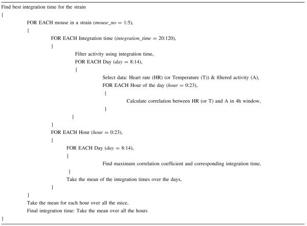
The aim of correlation analysis is to determine the time window for the activity data that provides the best correlation between integrated activity and temperature, and between integrated activity and heart rate. The analysis is applied to every mouse in each strain. The activity data are filtered over different time windows, which are chosen to be between 10 and 60 min in length (20–120 data points) with 10-min increments. After filtering the activity for the given time period (e.g., 10 min), the correlation between heart rate (or temperature) and activity is calculated for every hour of the day using a 4-h correlation window for each day in the experiment. The correlation window is chosen to be 4 h long in order to have a sufficient number of data points (Weinert and Waterhouse 1998). Because this correlation window is used for each hour, the 4-h intervals overlap, e.g., the first interval is 00:00:00 am-03:59:30 am, the second is 01:00:00 am-04:59:30 am. After calculating the correlation for each activity time window, the time window with the highest correlation is chosen for each hour of the day, and the mean of the lengths of the time window over all of the days of the experiment are calculated. As a result, we have mean activity time windows for every hour of the day for each mouse. Then, we calculate the mean activity time window for each hour by averaging over all the mice in a given strain. The final activity time window is then obtained by averaging over the hours.

The algorithm is summarized in Table 1 with example values in parentheses for the B6 males in Experiment 1.

Table 1.

Correlation analysis algorithm

The activity window lengths obtained from the correlation analysis are used to filter the activity data. In this work filtering refers to the integration of the activity data starting from the current point in time and going back in time as many time points as given by the length of the activity window. The filter structure (ARMA) is given by

$$\begin{array}{cc}\hfill a\left(1\right)y\left(n\right)=b\left(1\right)& x\left(n\right)+b\left(2\right)x(n-1)+\dots +b(n_b+1)\hfill \\ \hfill \times & x(n-n_b)-a\left(2\right)y(n-1)-\dots \hfill \\ \hfill \times & -a(n_a+1)y(n-n_a),\hfill \end{array}$$

where a(1) = 1, n_a = 1, b = 1,1,...,1, and n_b is equal to the number of points in the activity window. The filtering of the activity measurement is important because body temperature and heart rate are affected by the cumulative sum of activity rather than the spontaneous activity at a given point in time. The activity window length defines the time window where the integrated activity signal is highly correlated with the temperature and heart rate data.

Regression analysis

Regression analysis is used to obtain the heart rate and temperature circadian rhythms, as well as to test the sensitivities of heart rate and temperature rhythms to activity for different times of the day (Weinert and Waterhouse 1998). The analysis is applied to each individual mouse of the two strains studied. The activity data are first filtered using the filter lengths obtained using the correlation analysis discussed in the Correlation analysis subsection above, which are listed in Table 2. Then, a linear regression model is used to fit data between the heart rate and filtered activity data and between the temperature and filtered activity data for each hour of a 24-h period. For example, in the regression analysis between filtered activity and temperature, the activity and temperature data for each 1-h interval from every day in the experiment are selected, and a linear regression model is fit to these data. The same procedure is used to obtain linear models of heart rate with respect to the activity data. The gradients (slopes) of the linear regression models for each hour are used to quantify the sensitivity of temperature or heart rate to activity in that hour, and steeper slopes correspond to higher sensitivities. Sensitivity differences between the awake and sleep periods are tested for statistical significance using ANOVA (Devore 1991). Because they correspond to zero activity, the intercept from a regression curve represents the circadian rhythm for that mouse. The strain circadian rhythms are computed by averaging the circadian curves of individual mice over all the mice within a given strain.

Table 2.

Activity window lengths (min)

Strain	Exp 1 (HR)	Exp 1 (T)	Exp 2 (HR)	Exp 2 (T)
B6	34	76	43	73
A/J	36	68	40	68

T = temperature; HR = heart rate

Feature definition for temperature and heart rate rhythms

Feature definition for temperature circadian rhythm

Fourier analysis is used to identify a feature for the circadian temperature rhythms of the B6 and A/J mice that can be used to quantitatively characterize strain-specific behavior. The motivation for choosing Fourier analysis comes from a visual inspection of the circadian temperature curves in Fig. 2A. The temperature rhythms for the B6 males show a smoother transition between awake and sleep periods, whereas the rhythms for the A/J mice show a more abrupt change at these transitions and are essentially constant during the sleep period. Quantitatively, the smoother transition for the B6 mice is more analogous to a cosine wave-like characteristic than that of the A/J male and the rhythm for the A/J males has a temporal pattern that appears more like a square wave than a sinusoidal wave. This also suggests a more complex temperature rhythm for the A/J males compared to the B6 males because of the presence of additional spectral components in the time series. To quantify and use this observation as a feature, we use the fact that the Fourier spectrum of a cosine wave and a square wave can be distinguished by their harmonics. That is, a square wave has nonzero higher-order odd harmonics, which is not the case for a (pure) cosine wave. As a result, the ratio of the magnitude of the first harmonic to the third harmonic is smaller for a square wave when compared to that of a cosine wave. We use this ratio as a feature and test statistical significance of the differences between these harmonic ratios for the two strains using ANOVA. Note that the smooth versus sharp transitions in the temperature rhythm during the transitions between wake and sleep periods suggests a different regulatory mechanism for this rhythm between strains, and this is of biological interest.

Fig. 2.

(A) The intercepts of linear regression between temperature and activity: temperature circadian rhythms with mean ± SE. The intercepts are temperature values at zero activity; for this reason they are considered to be good estimates of the endogenous rhythm. (B) The gradients of linear regression between temperature and activity with mean ± SE. Gradients computed from the regression analysis determine the sensitivity of temperature to activity for different times of the day. The gradients (slopes) of the linear regression models for each hour are used to quantify the sensitivity of temperature to activity in that hour, and steeper slopes correspond to higher sensitivities

The Fourier series of a periodic signal is defined by (Oppenheim et al. 1996):

$$\begin{array}{c}x\left(t\right)=\sum _{k=-\infty }^{+\infty }{a}_k{e}^{jk{w}_{0}t}\hfill \\ a_k=\frac{1}{T_0}{\int }_{T_0}x\left(t\right)e^{-jk{w}_{0}t}dt\hfill \end{array}$$ (1)

Here, ω₀ is the fundamental frequency, and T₀ = 2π/ω₀ is the fundamental period. The coefficients a_k are called the Fourier series coefficients, and they quantify the complex amplitude of the signal at each harmonically related frequency of the signal. The constant component of the signal is given by a₀ for k = 0 and quantifies the DC component in the signal. The fundamental (first harmonic) components correspond to the terms with k = + 1 and k = −1. In general, the Nth harmonic components are the components for k = + N and k = −N. For a cosine wave, the Fourier coefficients are a₁ = a₋₁ = 1/2, and a_k = 0 otherwise. For a periodic square wave, where the signal is defined as

$$\begin{array}{cc}\hfill x\left(t\right)& =\{\begin{array}{cc}1,\hfill & \mid t\mid <T_1\hfill \\ 0,\hfill & T_1<\mid t\mid \le T_0∕2\hfill \end{array}\phantom{\}}\hfill \\ \hfill \text{and}& x(t+T_0)=x\left(t\right)\hfill \end{array}$$ (2)

the Fourier series coefficients are defined as a₀ = 2T₁/T₀, and

$$a_k=\frac{\sin k{\omega }_0{T}_1}{k\pi }\text{for}k\ne 0.$$

We see that for a pure cosine wave, the ratio of the magnitude of the coefficient of the first harmonic to the third is equal to infinity, whereas it is finite for a square wave. Thus, for the analysis of the circadian rhythm curves we expect the ratios for the B6 mice with a more cosine-like characteristic to be greater than the ratios for the A/J mice with a more square-wave-like characteristic.

Feature definition for heart rate rhythm

The heart rate data are analyzed using detrended fluctuation analysis (DFA) (Peng et al. 1995). Detrended fluctuation analysis is a widely accepted time-series analysis technique for the analysis of heart rate variability in the literature. Heart rate is a nonstationary signal and the variability in the signal is the result of both endogenous (biological) and exogenous (environmental) influences. One of the primary difficulties in the analysis of the heart rate signal is decomposing the variability into those components that result from environmental stimuli and those components that result from the underlying complexity of the (nonlinear dynamic) biological system. It is well understood that the fluctuations due to the underlying dynamical system show long-range correlations. Detrended fluctuation analysis is a technique that can be used to detect these long-term correlations in nonstationary heart rate data. The advantage of using DFA to detect these correlations is that it is effective in preventing the detection of false correlations that are artifacts of the nonstationarity behavior (Peng et al. 1995).

The DFA algorithm can be summarized as follows: The mean of the time-series data is first subtracted from the time-series data. The result is then integrated:

$$y\left(k\right)=\sum _{i=1}^k(d\left(i\right)-\stackrel{‒}{d}),$$

where d denotes the original data, and d‾ denotes the mean of the data. The integrated data are divided into boxes of equal length n. In each box, a least-squares regression line y_n(k) is computed to represent the trend of the data in that box. The integrated data are detrended by subtracting the local trend in each box, y(k) - y_n(k). The root-mean-square fluctuation of the integrated and detrended data is defined by

$$F\left(n\right)=\sqrt{\frac{1}{N}\sum _{k=1}^N{[y\left(k\right)-y_n\left(k\right)]}^2}.$$

The fluctuation function F(n) is computed for different box sizes n to find a relationship between F(n) and n. F(n) vs. n is then plotted on a double-log graph. If there is a linear relationship, this indicates the presence of power-law scaling in the time-series data. The scaling factor α is calculated as the slope of the linear curve relating log F(n) to log n. The scaling factor α varies between 0.5 (for uncorrelated data) and 1.5 (for Brownian noise). In the analysis of heart rate using DFA, we use the scaling factor α as the feature to identify differences between the B6 and A/J strains. The scaling factor a is a parameter that measures the self-similarity of a time series at different scales. If there is no self-similarity in the heart rate data, that is, the time series is more like a “white noise” process, then α will be equal to 0.5. For data with short-term self-similiarity, the initial slope of the log F(n) - log n plot can be different from 0.5, but the slope will approach 0.5 for large box sizes (n), indicating that on larger scales the signal is behaving similar to white noise. When 0.5 < α < 1, this shows persistent long-range power-law correlations where α = 1 corresponds to 1/f noise. If 0 < α < 0.5, this shows that there are power-law anticorrelations where small values are more likely to be followed by larger values and vice versa. When α ≥ 1, it shows that there are correlations in the data, but they are not in the form of a power law. α = 1.5 corresponds to Brownian noise (Peng et al. 1995).

Results

Correlation analysis results

Correlation analysis is used to analyze data from each strain of mice separately for the two experiments. The activity window lengths that give the best correlation between temperature (T) and activity and between heart rate (HR) and activity are summarized in Table 2. The distributions of the activity window lengths and the correlation coefficients between temperature and activity for Experiment 2 are shown in Fig. 3A, B to illustrate the results of the correlation analysis.

Fig. 3.

(A) Boxplots of the correlations between activity and temperature for Experiment 2. (B) Boxplots of the activity window lengths (for correlations between activity and temperature) for Experiment 2

For the activity window length that gives the best correlation between temperature and activity, the means of the correlation coefficients for the B6 mice are found to be between 0.48 and 0.81 during the awake period and between 0.69 and 0.81 during the sleep period. For the A/J mice, the coefficients are between 0.55 and 0.77 during the awake period and between 0.58 and 0.83 for the sleep period. The correlation coefficients are high during the sleep period compared to the awake period meaning that there is a stronger linear relationship between temperature and activity during the sleep period. These results agree with the results in the literature (Weinert and Waterhouse 1998), and the correlation coefficients in our work are higher than the coefficients given in this previous work. The biological interpretation for a strong linear relationship during the sleep period is explained and reviewed in Weinert and Waterhouse (1998). In particular, the reason for a weaker correlation between temperature and activity during the active (awake) period is attributed to the thermoregulatory mechanisms that are trying to avoid an excess rise in temperature due to high activity levels in this active phase. In the case of heart rate and activity, the correlation is found to be low for both strains of mice. For the B6 mice, the correlation coefficients are between 0.19 and 0.39 for the awake period and between 0.24 and 0.36 for the sleep period. For the A/J mice, the coefficients are between 0.41 and 0.57 for awake period and between 0.43 and 0.59 for sleep period. Because the linear relationship between heart rate and filtered activity is weak, for feature detection of the heart rate rhythms, we apply detrended fluctuation analysis to the raw heart rate data.

Results on the regression analysis between temperature and activity

In this section, we present the results of the regression analysis between temperature and activity for the B6 and A/J mice in Experiments 1 and 2. The mean circadian curves and gradients for each strain are computed by combining the results of all the mice of a given strain from both experiments, and then averaging over the mice. The resulting circadian temperature curves and gradients are shown in Fig. 2A, B. The lights are turned off at 18:00 and turned on at 06:00. When the B6 circadian rhythm curves are compared to the A/J curves, it can be observed that the B6 curves show a more cosine-like characteristic, whereas the A/J curves look more like a square wave. A quantitative measure of this strain-related difference is obtained using Fourier analysis as descibed in the subsection Feature definition for temperature circadian rhythm.

At present it is difficult to speculate about the molecular causes or consequences of these alternative waveforms. These differences suggest, however, that the biological regulation of temperature circadian rhythms may be significantly different in the A/J and B6 strains. Discovering the identity of the genes that control biological variation can provide clues to the molecular basis for the phenotypic trait and the mechanisms that coordinate patterns of change among functionally related traits. Similarly, because the mice within each strain are virtually identical, systematic studies can be undertaken in a cumulative manner to identify other traits that vary in a correlated manner, which will give further insight into the identification of functional relationships. A detailed characterization of traits such as circadian rhythms in various inbred strains is the first step in these studies. Single-gene mutations have been used in mice and other organisms to discover the molecular basis for circadian rhythms (King et al. 1997; Vitaterna et al. 1994). More recently, circadian rhythms have been discovered in many organs such as in adipose (Zvonic et al. 2006). Disturbances in these rhythms are associated not only with sleep disorders but also with metabolic disease (Turek et al. 2005) and xenobiotic metabolism (Green and Takahashi 2006). Moreover, mutations in genes whose conventional function involves energy metabolism also result in sleep disturbances (Laposky et al. 2006).

The intercepts that give the circadian rhythms are also obtained using second-order and third-order polynomial models to evaluate the effect of the model on the results. The intercepts are tested for their differences using ANOVA, and the results for both strains show that the null hypothesis cannot be rejected in either case, suggesting that the intercepts are not statistically different when different models are used (p = 0.0851 > 0.05 for the A/J mice, and p = 0.4776 > 0.05 for the B6 mice).

The differences between the sensitivities of temperature to activity for the sleep and awake periods are tested using ANOVA. The null hypothesis is that the mean gradients of the sleep period and the awake period are the same. The ANOVA test results show that the null hypothesis is rejected with p < 0.05 for B6 and not for A/J, where p = 5.3513 × 10⁻⁸ for the B6 males and p = 0.1668 for the A/J males. We then conclude that the sensitivities of temperature to activity are different for the awake and sleep periods for B6 mice. The differences in the sensitivities can also be observed from Fig. 2B, where the sensitivities are higher during the sleep period (06:00–18:00) than during the awake period for B6 mice. It should be noted that the mice sleep during the lights on period (06:00–18:00) and they are awake when the lights are off (18:00–06:00). The ANOVA test is also used to test the differences between the sensitivities of temperature to activity for sleep and awake periods for each individual mouse from each strain. The results for the B6 and A/J strains are given in Table 3. It is seen from the results that the group conclusion holds for individual B6 and A/J male mice, except for one B6 and two A/J mice.

Table 3.

ANOVA test results for comparing sensitivities between awake and sleep periods for B6 and A/J

	B6		A/J
Mouse No.	p value (T-A)	p value (HR-A)	p value (T-A)	p value (HR-A)
1	8.9 × 10−6	0.0009	0.2516	0.0753
2	1.4 × 10−5	0.0001	0.0906	0.4223
3	1.1 × 10−4	0.0003	0.1611	0.7124
4	3 × 10−5	0.0007	0.0413	0.2436
5	0.08	0.0847	0.0242	0.0766
6	0.009	0.0685	0.4275	0.6723
7	4 × 10−6	0.151	0.4744	0.6205
8	0.002	0.6595	0.0913	0.3167
9	0.0151	0.0294	0.1086	0.1766
10			0.0556	0.03
11			0.9115	0.1439
12			0.1377	0.0043
	Mean: 0.0118	Mean: 0.1106	Mean: 0.2313	Mean: 0.2912
	SD: 0.0261	SD: 0.2123	SD: 0.2591	SD: 0.2575

T-A = temperature-activity; HR-A = reart rate-activity

Results of the feature definition for temperature circadian rhythm

For each mouse in each strain from both Experiments 1 and 2, we first compute the Fourier series coefficients and then compute the ratio of the coefficients of the first harmonic to the third harmonic. From our visual analysis, it is expected that the ratios for the B6 males will be higher than the corresponding ratios for the A/J males because of the presumed resemblance to cosine- and square-wave-like rhythms. The results summarized in Table 4 show that in fact the ratios for the B6 males are higher than those for A/J males. The strain differences for the ratios are tested using ANOVA, and the result shows that the means of the ratios are significantly different from each other for the two strains with p = 0.0139 < 0.05, and the two strains are clearly separated from each other. The results also confirm that the ratio of the Fourier coefficients can be used as a feature to characterize this strain-specific behavior, and it can further be used to test the behavior of consomic mice to identify their behavior similarities or differences to the progenitor strains, B6 and A/J. These results will be presented in a subsequent publication.

Table 4.

Ratios of the Fourier series coefficients (first/third)

Mouse No.	B6	A/J
1	6.8899	2.7392
2	3.0875	2.619
3	4.0115	2.1461
4	3.5923	1.8277
5	3.3091	3.8156
6	7.1701	4.5102
7	5.716	3.2178
8	3.8574	2.3084
9	2.1368	3.0133
10		3.1446
11		2.2334
12		3.1336
	SE: 0.5861	SE: 0.2180

To show that the use of the ratios of the Fourier coefficients as a feature is not a biased feature with respect to the different filter lengths used for each strain, we have used the same filter length for both strains (filter length = 68), and we have calculated the ratios of the Fourier coefficients for this case. The strain differences for the ratios are also tested using ANOVA, and the result shows that the means of the ratios are significantly different from each other for the two strains with p = 0.0131 < 0.05. This result shows that the feature is not biased with respect to the use of different filter lengths for each strain, and that this feature can be used to identify strain differences. The reason for using strain-specific filter lengths is to eliminate the majority of the exogenous activity effect from the temperature and heart rate data, thereby allowing a more accurate analysis of the circadian rhythms associated with each strain. The coefficient of variation (CV) is also calculated for the ratios of both strains. The CV is found to be 0.2611 for the A/J mice and 0.3979 for the B6 mice. The low CV values also show that the feature is not biased.

Results on the regression analysis between heart rate and activity

The heart rate circadian rhythms are generated as the intercepts of the linear regression curves between heart rate and activity for the B6 and A/J mice of Experiments 1 and 2. The mean circadian curves and gradients for each strain are again computed by averaging the individual mice curves and gradients over all the mice in a given strain. The resulting circadian heart rate curves and gradients are shown in Fig. 4A, B. The heart rate circadian rhythms of the A/J mice show a clear cycling between the sleep and awake periods, and this difference cannot be observed for the B6 mice. The B6 intercepts have a peak just when the lights are turned off at 18:00, and they stay almost constant during the day.

Fig. 4.

(A) The intercepts of linear regression between heart rate and activity: heart rate circadian rhythms with mean ± SE. The intercepts are heart rate values at zero activity; for this reason they are considered to be good estimates of the endogenous rhythm. (B) The gradients of linear regression between heart rate and activity with mean ± SE. Gradients computed from the regression analysis determine the sensitivity of heart rate to activity for different times of the day. The gradients (slopes) of the linear regression models for each hour are used to quantify the sensitivity of heart rate to activity in that hour, and steeper slopes correspond to higher sensitivities

The differences between the sensitivities of heart rate to activity for the sleep and awake periods are also tested using ANOVA, where the null hypothesis is again the equivalence of the means in these two periods. The ANOVA test results show that the null hypothesis is rejected for p < 0.05 for B6 mice and not for A/J, where p = 5.3051 × 10⁻⁶ for B6 males and p = 0.1863 for A/J males. It can then be concluded that the sensitivities of heart rate to activity are different for the awake and sleep periods for B6 mice. The null hypothesis is not rejected for the A/J males, indicating that it cannot be concluded that the sensitivities are different for the sleep and awake times. It can also be observed from Fig. 4B that the sensitivities are higher during the sleep period (06:00–18:00) for B6 mice.

The ANOVA test is also applied to each individual mouse from each strain to test the difference between the sensitivities of heart rate to activity for the sleep and awake periods. The results for the B6 and A/J strains are given in Table 3. It is seen from the results that the group conclusion holds more generally for individual A/J male mice than for individual B6 male mice.

Results of the feature definition for heart rate rhythm

Detrended fluctuation analysis is used to analyze the raw heart rate time-series data for each mouse from each strain in Experiments 1 and 2. The scaling factor α is calculated as the gradient of the linear regression analysis between log F(n) vs. log n. The α values for each strain are summarized in Table 5. For B6 mice, the α values are between 0.5 and 1, except for one mouse with α = 1.0038. This shows that the heart rate data for B6 mice have persistent long-range power-law correlations. The α values for A/J mice are all greater than 1, except for two mice that have α values very close to 1. This shows that the heart rate data for the A/J mice have correlations that are not of the power-law type. This provides a more detailed analysis of heart rate variability and also possibly suggests that there are different biological mechanisms involved in the regulation of heart rate between these two strains. The differences between the means of the scaling factors of the strains are tested using ANOVA, and the result shows that they are significantly different, with p = 6.591 × 10⁻⁵ < 0.05, confirming that the scaling factor is a feature that can be used to distinguish between the strain-specific behavior of the heart rate rhythms.

Table 5.

Scaling factors (α)

Mouse No.	B6	A/J
1	0.9038	1.0389
2	0.8866	1.1259
3	0.8559	0.9975
4	0.7653	1.0101
5	0.9718	1.0987
6	0.8343	1.0783
7	0.903	1.0158
8	1.0038	1.044
9	0.9172	0.962
10		1.2205
11		1.0343
12		1.2322
	Mean: 0.89	Mean: 1.072
	SD: 0.07	SD: 0.085
	CV: 0.0796	CV: 0.0792
	SE: 0.0237	SE: 0.0245

Discussion

In this article we have analyzed telemetric heart rate, temperature, and activity data for two strains of inbred mice (B6 and A/J) to characterize the strain-specific behavior of the circadian rhythms of the heart rate and temperature time series. The activity effect is eliminated from both the heart rate and temperature time series using correlation analysis followed by linear and polynomial regression analysis. The circadian curves are obtained as the intercepts of the linear and polynomial regression curves. The regression analysis is used to provide the sensitivities of the heart rate and temperature time series to activity for different times of the day. We have tested the difference between the sensitivities for the awake and sleep periods for statistical significance and the results show that for a p < 0.05 test, the sensitivities of both the heart rate and temperature to activity are different for the sleep and awake periods for B6 mice. The A/J males do not show statistically significant differences in the sensitivities for both the heart rate and temperature circadian rhythms.

The temperature circadian rhythms for the B6 males were found to have a more cosine-like temporal characteristic, whereas the temporal rhythms for the A/J males were more like a square wave. Based on this observation, we defined a distinguishing feature using Fourier analysis as the ratio of the magnitude of the Fourier coefficient of the first harmonic to the magnitude of the Fourier coefficient of the third harmonic. The results of this analysis showed that there are higher ratios for B6 males than for A/J males. This confirms that the B6 strain characteristic is closer to a cosine-like waveform than the A/J strain. The statistical tests also showed that using this feature the strains can be separated from each other with high statistical significance. Although the exact biological underpinning for this finding is not known, it does suggest that the B6 and A/J strains have different regulation mechanisms for circadian temperature rhythms. This observation, as quantified by the spectral ratio defined in this work, may provide a useful starting point for further analysis in consomic mice experiments with the objective of isolating the genes that are responsibe for this regulation mechanism. Our future work is directed at such investigations.

Heart rate rhythms are analyzed using detrended fluctuation analysis, and the power-law scaling factor α in this analysis is used as the feature to analyze strain-dependent differences in the heart rate rhythms. The statistical test results in this case also showed that using this feature we are able to separate strain-specific behavior with high statistical significance. The two features defined in this work for the temperature and heart rate circadian rhythms enable characterization of strain-specific behavior, which can be used further to identify behavioral changes with respect to temperature and heart rate rhythms in consomic mice.

The analysis of intrastrain variability is limited to the results presented in Tables 3-5. In Table 3, ANOVA is used to test the difference between the sensitivities of temperature to activity and heart rate to activity for the B6 and A/J strains during sleep and awake periods. We observed that the results for individual mice from each strain are consistent with the group (B6 and A/J strains) results in 8 out of 9 individual mice for the B6 and 10 out of 12 individual mice for the A/J. Results for characterizing the circadian temperature for the B6 and A/J mice and strains are summarized in Table 4. The feature chosen is the ratio of first to third harmonic (B6 mean = 4.42, standard deviation = 1.76; A/J mean = 2.9, standard deviation = 0.76), with standard errors for each strain given in the table. Clearly, this feature is able to distinguish between the strains in a statistically significant manner with intravariability with coefficient of variation (CV) equal to 0.4 for the B6 and 0.26 for the A/J. The results for the sensitivities of heart rate to activity are not as good and hence we use detrended fluctuation to study the intra- and interstrain characteristics. Table 5 summarizes these results.

Our work highlights distinct patterns of coordination of physiologic systems in different strains. We have found that the temperature and heart rate rhythms for B6 and A/J mice are different and can be used to distinguish the strains from each other with high statistical significance. The genetic, molecular, and physiologic bases for variation in each of these traits and the basic differences in coordinating mechanisms remain to be determined. These strains and the chromosomal substitution strains derived from them, together with the analytical methods that we present here, provide a foundation for discovering the genetic and mechanistic basis for fundamental control aspects in complex biological systems.

The analytical methods presented here estimate the genetic versus nongenetic component of phenotypic variation. Analysis of this type is commonly done in populations where the genetic contribution to phenotypic variation is not evident. Before genetic studies are undertaken in these cases, heritiability is estimated to provide evidence that genetic studies are justified. In studies with inbred strains, evidence for a genetic component is simply a significant difference between the strains being studied. The mice are raised in a uniform environment and therefore phenotypic differences are attributed to genetic variation.

The cardiovascular traits for the B6 and A/J mice are studied using telemetry in Hoit et al. (2002) together with an analysis of the relationships among activity, heart rate, and temperature. The data analyzed in our article are similar to those in the study by Hoit et al. (2002), and the observations that all three traits have similar patterns of temporal variation in both the B6 and A/J and that the A/J mice have a higher heart rate and lower body temperature than the B6 mice also apply here. It is also discussed in Hoit et al. (2002) that temperature is strongly correlated with activity in both strains, while the correlation between heart rate and activity is relatively weak. Our correlation analysis results agree with these earlier observations as we have also found that the correlation between temperature and activity is high, whereas the correlation between heart rate and activity is low. The blood pressure and heart rate rhythms in C57BL mice were studied in Li et al. (1999) using carotid arterial catheters. They found that heart rate has a maximal value that was evident during the early part of the dark (awake) phase. The heart rate rhythms in our results for the B6 mice shown in Fig. 4A also have a maximum peak right after the lights are switched off, which agrees with the earlier results given in Li et al. (1999).

A similar study on circadian rhythms using telemetry data was conducted in Tankersley et al. (2002). They studied the variability in the circadian rhythms of activity, body temperature, and heart rate between C3H/HeJ and C57BL/6J (B6) mice. The objective was to analyze the genetic factors modulating the variation in the circadian rhythms. The difference between our methodology and theirs is that they do not take into account the effect of activity on the heart rate and temperature rhythms. Their analysis is based on a statistical model where a periodic function for each rhythm (heart rate, activity, and temperature) is estimated. They then used this model to compare the differences in the circadian patterns and as such there is no feature identification in their work. In our work, we eliminated the effect of activity from the heart rate and temperature rhythms, and then we compared the resulting circadian rhythms by defining features that enable the successful separation of the two strains based on strain-specific behavior.

Pattern recognition within and between individuals and strains and before and after perturbations is a major challenge in the study of temporal changes in biological systems. These challenges include general trends as well as signals from specific events. High-density data streams, such as those studied here, can provide the information that is needed to study the fine structure of temporal changes. But the “noise” associated with stochastic events can seriously complicate the detection of meaningful signals. The work reported here is a step toward resolving this problem. Being able to effectively and efficiently deal with intra- and interstrain variability in a statistically meaningful way is necessary for future work aimed at dissecting the details associated with the temporal control of various biological rhythms and processes, e.g., a study of functional genomics with consomic mice. In a translational research setting, we can imagine the use of telemetric sensor systems and networks with appropriate signal processing and feature extraction with the ability to recognize significant biological events providing monitoring and perhaps the anticipation of critical events in at-risk individuals.

References

- Devore JL. Probability and statistics for engineering and the sciences. 3rd edn. Brooks/Cole Publishing Co; Pacific Grove, CA: 1991. [Google Scholar]
- Green C, Takahashi J. Xenobiotic metabolism in the fourth dimension: partners in time. Cell Metab. 2006;4(1):3–4. doi: 10.1016/j.cmet.2006.06.002. [DOI] [PMC free article] [PubMed] [Google Scholar]
- Hoit B, Kiatchoosakun S, Restivo J, Kirkpatrick D, Olszens K, et al. Naturally occurring variation in cardiovascular traits among inbred mouse strains. Genomics. 2002;79(5):679–685. doi: 10.1006/geno.2002.6754. [DOI] [PubMed] [Google Scholar]
- King DP, Zhao Y, Sangoram AM, Wilsbacher LD, Tanaka M, et al. Positional cloning of the mouse circadian clock gene. Cell. 1997;89(4):641–653. doi: 10.1016/s0092-8674(00)80245-7. [DOI] [PMC free article] [PubMed] [Google Scholar]
- Laposky AD, Shelton J, Bass J, Dugovic C, Perrino N, et al. Altered sleep regulation in leptin-deficient mice. Am J Physiol Regul Integr Comp Physiol. 2006;290(4):894–903. doi: 10.1152/ajpregu.00304.2005. [DOI] [PubMed] [Google Scholar]
- Li P, Sur S, Mistlberger R, Morris M. Circadian blood pressure and heart rate rhythms in mice. J Physiol. 1999;276(2 Pt 2):R500–R504. doi: 10.1152/ajpregu.1999.276.2.R500. [DOI] [PubMed] [Google Scholar]
- Nadeau J, Singer J, Matin A, Lander E. Analyzing complex traits with chromosome substitution strains. Nat Genet. 2000;24:221–225. doi: 10.1038/73427. [DOI] [PubMed] [Google Scholar]
- Oppenheim A, Willsky A, Nawab S. Signals and systems. 2nd edn. Prentice-Hall; Upper Saddle River, NJ: 1996. [Google Scholar]
- Peng C, Havlin S, Stanley H, Goldberger A. Quantification of scaling exponents and crossover phenomena in nonstationary heartbeat time series. Chaos. 1995;5:82–87. doi: 10.1063/1.166141. [DOI] [PubMed] [Google Scholar]
- Tankersley C, Irizarry R, Flanders S, Rabold R. Circadian rhythm variation in activity, body temperature, and heart rate between c3h/hej and c57bl/6j inbred strains. J Appl Physiol. 2002;92(2):870–877. doi: 10.1152/japplphysiol.00904.2001. [DOI] [PubMed] [Google Scholar]
- Turek FW, Joshu C, Kohsaka A, Lin E, Ivanova G, et al. Obesity and metabolic syndrome in circadian clock mutant mice. Science. 2005;308(5724):1043–1045. doi: 10.1126/science.1108750. [DOI] [PMC free article] [PubMed] [Google Scholar]
- Vitaterna MH, King DP, Chang AM, Kornhauser JM, Lowrey PL, et al. Mutagenesis and mapping of a mouse gene, clock, essential for circadian behavior. Science. 1994;264(5159):719–725. doi: 10.1126/science.8171325. [DOI] [PMC free article] [PubMed] [Google Scholar]
- Weinert D, Nevill A, Weinandy R, Waterhouse J. The development of new purification methods to assess the circadian rhythm of body temperature in Mongolian gerbils. Chronobiol Int. 2003;20(2):249–270. doi: 10.1081/cbi-120018649. [DOI] [PubMed] [Google Scholar]
- Weinert D, Waterhouse J. Diurnally changing effects of locomotor activity on body temperature in laboratory mice. Physiol Behav. 1998;63(5):837–843. doi: 10.1016/s0031-9384(97)00546-5. [DOI] [PubMed] [Google Scholar]
- Zvonic S, Ptitsyn AA, Conrad SA, Scott LK, Floyd ZE, et al. Characterization of peripheral circadian clocks in adipose tissues. Diabetes. 2006;55(4):962–970. doi: 10.2337/diabetes.55.04.06.db05-0873. [DOI] [PubMed] [Google Scholar]