Mueller matrix retinal imager with optimized polarization conditions

Abstract

A new Mueller matrix polarimeter was used to image the retinas of normal subjects. Light from a linearly polarized 780 nm laser was passed through a system of variable retarders and scanned across the retina. Light returned from the eye passed through a second system of retarders and a polarizing beamsplitter to two confocal detection channels. Optimization of the polarimetric data reduction matrix was via a condition number metric. The accuracy and repeatability of polarization parameter measurements were within ± 5%. The magnitudes and orientations of retardance and diattenuation, plus depolarization, were measured over 15° of retina for 15 normal eyes.

1. Introduction

Glaucoma, age-related macular degeneration, and diabetic retinopathy are responsible for 25% of blindness worldwide [1]. These diseases can cause complex changes to the retina that are often difficult to detect early enough to ensure effective treatment [2–4]. With disease, the retinal tissue becomes disordered, in contrast to the well-ordered layers of the healthy retina, and thus they differ in their interaction with polarized light [5].

More sensitive diagnostic tests could potentially be developed using the interaction of polarized light with retinal tissue, exploiting subtle changes in retinal and choroidal microstructure. The more ordered a structure, the larger the expected diattenuation and retardance. As these cellular structures become disordered in certain disease states, the diattenuation and retardance would be expected to decrease and the depolarization would be expected to increase. Previously, incomplete polarimeters have been used to probe the increase of scattered light concomitant with retinal disease [5–8], demonstrating the utility of depolarization images to provide contrast for deep tissue scattering abnormalities in age-related macular degeneration, central serous chorioretinopathy, and other maculopathies. Polarimeters such as the Carl Zeiss Meditec (formerly Laser Diagnostics) GDx have been used to quantify changes to the retinal ganglion cell axons in glaucoma, by measuring the linear retardance of the nerve fiber layer. The GDx, as an incomplete polarimeter, does not measure all three forms of polarization behavior: depolarization, diattenuation, and retardance. Thus its retardance measurements are increasingly inaccurate as depolarization and diattenuation increase [9].

The overall thickness of the retina ranges from 50 μm at the foveal pit to 600 μm at the optic nerve head, with different layers changing in thickness as a function of distance from the fovea. At the center of the fovea, the superficial retinal layers are displaced eccentrically, leaving only cone cells with their axons radiating outwards in the Henle fiber layer towards synapses with bipolar cells. Where the retinal tissue has at least partial structural regularity over the measurement volume, collective magnitude and phase modifications to incident polarized light accrue and are measured as (respectively) diattenuation and retardance. The measured values are specific to the tissue structure. However, when the structure has low structural regularity over the measurement volume, the magnitude and phase modifications vary significantly. Lacking a collective magnitude and phase change, the measurement indicates depolarization. Multiple tissue layers in the light path with multiple polarization effects all contribute to the polarization interaction.

Structures with the most regular microstructure and thus most likely to generate non-depolarizing polarization effects are: the stroma in the cornea; the retinal nerve fiber layer; the lamina cribrosa and scleral crescent at the ONH; Henle’s fiber layer in the retina; the rod and cone photoreceptors; Bruch’s membrane; and the sclera [8]. The strongest polarization effects are found in the cornea, retinal nerve fiber layer, and Henle’s layer [10]. These anisotropic structures contain long thin parallel-oriented cylinders (such as collagen fibrils or microtubules), uniformly distributed within the surrounding medium, and with dimension smaller than the wavelength of visible light. Models have been developed to describe diattenuation and retardance effects when polarized light interacts with structured ocular tissues [11,12]. Though models of this type are useful for predicting the general types of polarization effects to be found in ocular tissues based on their structure, they have limited application in quantifying the magnitude of the effects due to strong dependencies on ocular variables which are difficult to specify accurately, such as spatial distributions of refractive indices, cylinder size, and packing density.

Direct measurements of retinal polarization properties have been made using a variety of techniques. The Mueller matrix ellipsometry technique reported in 1985 by van Blokland [13] was the first method to use a complete Mueller matrix polarimeter together with analysis methods based on the Mueller calculus and Poincaré sphere trajectories; this work set the stage for later research efforts. Though non-imaging, this approach provided a full Mueller matrix of individual retinal locations and demonstrated significant retinal depolarization. To determine polarization properties over a wider retinal region, imaging methods have since been developed including camera-based polarimeters [9] and scanning laser polarimetry (SLP) [14–16]. The accuracy of these methods depends on the configuration of the polarimeter generator (polarization components in the outgoing path) and analyzer (polarization components in the incoming path). An incomplete polarimeter configuration must be inaccurate when the collected light has polarization content in a direction lying outside the polarimeter’s measurement space; this energy is coupled as error into the measurable polarization components [17]. For example, the Carl Zeiss Meditec GDx is an incomplete polarimeter with a measurement space which includes retardance but not depolarization or diattenuation. Given that ocular interactions are partially depolarizing, particularly in older and surgically altered eyes [9, 18], the GDx retardance measurement must be inaccurate to some degree. Bueno has observed this inaccuracy to be significant and correlated with degree of polarization in a study involving subjects displaying varying levels of ocular depolarization [9].

Mueller matrix imaging polarimetry (MMIP) uses a polarimeter that is complete so that a full Mueller matrix is obtained at every point in a retinal image. MMIP in a camera-based configuration has been used to quantitatively measure polarization in the in vitro cornea [19] and lens [20] and in the in vivo full eye [21]. MMIP in the SLP configuration has been reported in the context of image quality improvement and enhanced contrast for retinal features [22,23]. Lara and Dainty [24] have reported a complete polarimeter configuration using multiple detection channels; this instrument is in early development and requires manual translation to produce a two-dimensional image. MMIP techniques require the collection of at least 16 images at different polarimeter states, typically over a wide intensity range within the image set. Reported MMIP instruments have been limited by the need to manually adjust polarization components, slow data acquisition time (lens paralysis or pupil dilation has been required), difficulty in co-registering images, and inadequate dynamic range.

The imaging Mueller matrix retinal polarimeter described here was developed to obtain high quality retinal images in vivo to measure the full 16 degrees of freedom in the Mueller matrix. This polarimeter, referred to as the GDx-MM (MM for Mueller Matrix), is based on modifications to a commercially available scanning laser polarimeter, the GDx (the GDx used in this study was manufactured by Laser Diagnostics). Using the GDx-MM all polarization parameters (retardance, diattenuation, and depolarization) are measured independently and simultaneously. The GDx-MM is completely automated, recording 72 polarization images with 20 μm resolution over a 15° visual field in 4 seconds. Lens paralysis and pupil dilation are not required. The polarimeter design is optimized for good performance in the presence of known error sources. In this paper, the GDx-MM instrument design is discussed, including design requirements, optimization methods, calibration, data processing, and validation. Representative polarization parameter images from a study on normal human subjects are presented and discussed.

2. Methods

2.1 Experimental system

The original GDx is a SLP with a linearly polarized 780 nm laser source, a rotating half wave plate, and a polarizing beamsplitter which directs the co- and cross- polarized return light to two detection channels. A two-dimensional retinal scan is performed for each of 20 waveplate orientations. The signals from the co- and cross-polarized detectors are processed to produce a linear retardance map of the scanned region. A constant birefringence factor converts the retardance map to a thickness map of the retinal nerve fiber layer. The resolution at the retina is about 15 μm, and the scan covers a visual field of 15°. Scanning is via a slow scan galvanometer driven at 26 Hz coupled to a fast resonant scanner oscillating at 4 kHz. The data presented in this paper is from the co-polarized channel only.

Complete Mueller matrix polarimetry requires at least 16 measurements, utilizing linearly independent combinations of generator and analyzer polarization states. Typical methods to create these states include polarizers in combination with retardation elements, which may include retarders on rotary stages, liquid crystal variable retarders, electro-optic modulators, or photoelastic modulators. Space is very limited within the GDx and thus our choice was to install two liquid crystal variable retarders (LCVRs), one in the generator path and one in the analyzer path. The generator and analyzer states are then determined by combinations of the LCVR retardances and the rotating waveplate orientation. Fig. 1 shows the GDx-MM optical and polarization path with modifications from the original GDx. The instrument is more fully described in [25].

Fig. 1.

GDx-MM optical and polarization path. NPBS: non-polarizing beamslitter; PBS: polarizing beamslitter; APD: avalanche photodiode; LCR: liquid crystal retarder. Modifications from the GDx path are emphasized in red and include the following: insertion of LCR-G in generator path; insertion of LCR-A in analyzer path; and changing the retardance and rotational increment of the rotating waveplate.

The use of LCVRs in polarimetric applications is well established [26,27]. Although LCVRs have small size and adjust retardance at low voltage, they have significant disadvantages which adversely affect the polarimeter accuracy. (1) The retardance drift with temperature is large, approximately 0.5% per ºC. (2) The retardance varies rapidly with angle of incidence. (3) The response time is slow, tens of milliseconds. (4) There is significant scatter and nonuniformity across the liquid crystal aperture which introduces noticeable amounts of depolarization. Our LCVRs have a 3º change in retardance per degree in angle of incidence. The response time is 30–80 ms, and depolarization index is 0.01.

2.2. Optimization of polarimeter design

The GDx-MM generator and analyzer states were selected through consideration of Poincaré sphere trajectories and by minimization of the polarimetric measurement matrix condition number [17]. A Mueller matrix polarimeter illuminates the sample with a series of generator states (Stokes vectors) g_i and analyzes the light which has interacted with the sample with a set of analyzer states a_i recording a set of flux measurements arranged in a vector P. The polarimeter is represented by the polarimetric measurement matrix W where each row w_i is given by:

$$w_i=[\begin{array}{ccccccc}{a}_{i,0}{g}_{i,0}& a_{i,0}{g}_{i,1}& a_{i,0}{g}_{i,2}& a_{i,0}{g}_{i,3}& a_{i,1}{g}_{i,0}& \cdots & a_{i,3}{g}_{i,3}\end{array}].$$ (1)

The sample Mueller matrix M is calculated from P as a linear least squares estimation process using the established polarimetry equations [28]

$$\mathbf{WM}=\mathbf{P}{\mathbf{W}}^{-\mathbf{1}}\mathbf{P}=\mathbf{M},$$ (2)

where the pseudo-inverse is preferred when W is not square.

For the GDx-MM the optimizable parameters are the LCVR retardances and orientations and the rotating waveplate retardance and angular increment. To perform this optimization, the generator and analyzer were expressed as composite Mueller matrices with the retardances and orientations as optimization parameters. A polarimeter state sequence of rotating the waveplate several increments for each of several LCVR retardance values was established by considering that the LCVR response time is significantly longer than the waveplate rotation time. The sequence duration is limited by consideration of typical eye movement and blinking patterns; a maximum measurement time of four seconds was selected. The full sequence consists of four sets of fixed LCVR retardances, with 18 rotating waveplate positions per set, for a total of 72 states. Optimization was begun via a Poincaré sphere analysis identifying parameter values which minimize the maximum distance from any point on the sphere to that trajectory. The analysis showed that to form a rank 16 polarimetric measurement matrix with good coverage of the sphere: (1) the GDx rotating half wave plate should be replaced by one with a lower retardance; (2) this waveplate should rotate twice as far (through 90° rather than 45°); and (3) the LCVRs should be oriented at 45°.

A stability analysis utilizing condition number was performed to determine optimal retardances; this is a standard technique used by many researchers to design polarimeters with improved stability in the presence of error [17,29,30]. To perform our condition number analysis each variable in W was varied, and the values yielding the W with lowest L₂ condition number κ₂(W) was selected. κ₂(W) is defined as the product of the L₂ norms of W and its inverse:

$${\kappa }_2(\mathbf{W})={\Vert \mathbf{W}\Vert }_2{\Vert {\mathbf{W}}^{-1}\Vert }_2,\text{where}{\Vert \mathbf{A}\Vert }_2=\underset{x}{sup}\frac{{\Vert \mathbf{A}x\Vert }_2}{{\Vert x\Vert }_2}.$$ (3)

The L₂ condition number also equals the ratio of the largest to smallest singular values in the singular value decomposition of W.

Our optimized polarimeter configuration is summarized in Table 1. For each of four groups, the generator and analyzer LCVRs have fixed retardance combinations selected from 3/8, 5/8, and 7/8 wave (multiple combinations giving minimum condition number exist). Within each group, the waveplate rotates in 4.864° increments for a total rotation of 87.5° (the increment size is constrained by the GDx motor drive). The optimized rotating waveplate retardance was 145°. This configuration gives a rank 16 polarimeter with an L₂ condition number of 14.5 (sixteen singular values ranging from 9.4 to 0.6), comparable to that of a dual rotating retarder polarimeter [29]. By comparison, the GDx is a rank 8 polarimeter with eight singular values ranging from 7.4 to 0.4. A comparison of the trajectories of each polarimeter’s generator on the Poincaré sphere demonstrates that the accessible portion of the sphere is significantly greater for the GDx-MM (Fig. 2).

Table 1.

GDx-MM Polarimeter States

Group:States	Generator LCVR retardance	Analyzer LCVR retardance	LCVRs orientation	Rotating waveplate retardance	Rotating waveplate orientation
1: 1–18	7/8 wave	5/8 wave	45°	145°	0°–87.5°
2: 19–36	7/8 wave	5/8 wave	45°	145°	90°–177.5°
3: 37–54	5/8 wave	3/8 wave	45°	145°	180°–267.5°
4: 55–72	3/8 wave	7/8 wave	45°	145°	270°–357.5°

Fig. 2.

Generator trajectories on the Poincare sphere. (a): GDx trajectory is limited to one half of the equator, and thus cannot measure elliptical or circular polarization. (b): GDx-MM trajectory covers a substantially larger portion of the sphere; shown are different trajectories corresponding to the set of LCVR retardances.

LCVRs were supplied by Bolder Vision Optik, Boulder, CO. A zero-order 145° birefringent polymer waveplate was obtained from Meadowlark Optics, Frederick, CO. The GDx electronics were replaced with a custom data acquisition and control system [National Instruments, Austin, TX]. More detail may be found in [25].

2.3. Calibration

Calibration was performed by direct measurement of each polarimeter state using external calibrated polarimeters. In a novel approach to calibration, data was collected for all possible combinations of rotating waveplate orientation (from 0° to 87.5° in 4.864° increments) and LCVR retardance (in the set {3/8, 5/8, 7/8 wave}). All possible polarimetric measurement matrices were formed from the large number of calibrated states, and the associated L₂ condition number of each was calculated. The W with the lowest L₂ condition number (of about 15.1) was identified, and the corresponding combination of states was chosen. This approach provides improved measurement accuracy in the presence of error.

A data reduction algorithm converted raw data into sets of 72 retinal images. These images were co-registered to compensate for saccadic eye movement and/or blinking during the scan. A Mueller matrix was then calculated at each pixel via W. Individual images could be dropped from the data set due to blinking, excessive eye movement, or the presence of artifacts such as tear films; in this case the corresponding rows from W are deleted, W_P⁻¹ is recomputed, and data reduction proceeds with a reduced image set.

Due to noise, M is often not a physically realizable (“physical”) Mueller matrix, i.e. for some input Stokes vectors the degree of polarization is less than zero or greater than one, or the intensity is negative. To ensure accurate extraction of polarization parameters such as retardance, the nearest physical Mueller matrix M′ is first found. Two methods have been applied with similar results. In both methods M is first converted to a Hermitian matrix H:

$$\mathbf{H}=\frac{1}{2}\sum _{i=0}^3\sum _{j=0}^3{m}_{ij}{\sigma }_i\otimes {\sigma }_j,$$ (4)

where m_ij are the elements of M, ⊗ indicates the outer product and the σ’s are the normalized Pauli spin matrices:

$${\sigma }_0=\left(\begin{array}{cc}1& 0\\ 0& 1\end{array}\right),{\sigma }_1=\left(\begin{array}{cc}0& 1\\ 1& 0\end{array}\right),{\sigma }_2=\left(\begin{array}{cc}0& -i\\ i& 0\end{array}\right),{\sigma }_3=\left(\begin{array}{cc}1& 0\\ 0& -1\end{array}\right).$$ (5)

Physical M yield H with positive eigenvalues; non physical M have one or more negative eigenvalues. When M is non physical, the eigenvalues of H are used as the starting point for a new Hermitian matrix H′. In one method based on [31], the normalized Cholesky decomposition of H′ is used to determine a non-negative eigenvalue set. In an alternate method having faster processing time but lower accuracy in some cases, all negative eigenvalues of H are zeroed and H′ is formed per the eigen decomposition theorem from the eigenvectors of H. M′ is reconstructed from H′ as

$$m_{ij}^{\prime }=Tr\left\{{\mathbf{H}}^{\prime }\lfloor {\sigma }_i\otimes {\sigma }_j^{\ast }\rfloor \right\},$$ (6)

where Tr is the trace function.

Each M′ is decomposed into diattenuation, retardance, and depolarization component matrices via the Lu-Chipman algorithm [32]. Polarization properties of interest such as retardance magnitude and orientation are calculated on a per-pixel basis from the appropriate component matrix, and then assembled into “polarization parameter” images showing how each parameter varies spatially across the imaged portion of the retina. All data processing steps were performed using custom applications written in Labview, Mathematica [Wolfram Research Inc., Champaign, IL], and Matlab [The Mathworks, Natick, MA].

2.4. Validation

Known error sources reduce the accuracy of the GDx-MM. Systematic (nonzero mean) sources include uncertainty in the rotating waveplate start position (± 1 motor step: ± 2.432º), temperature-induced retardance drift of the LCVRs (0.5% per ºC), and temperature-induced gain drift in the avalanche photodiode detectors (3% – 5% per ºC). Random (zero mean) sources include uncertainty in the waveplate incremental rotation (± 0.1º) and the Poisson-distributed shot noise in the avalanche photodiode detectors. For a temperature range of ± 5ºC, a simulation predicts that the GDx-MM should have absolute worst case error of 0.25 in diattenuation magnitude, 6º in diattenuation orientation, 0.15 rad in retardance magnitude, 5º in retardance orientation, and 0.2 in depolarization index. Highest error contribution is from the waveplate start position and the LCVR retardance drift with temperature. In an ideal case where the waveplate starts properly at position zero and the instrument is used within ± 1º of the calibration temperature, the predicted error is about five times lower than these worst case values.

A validation procedure was performed by measuring the Mueller matrices of known standards including a polarizer, two waveplates, and a depolarizer. This was done to demonstrate typical accuracy of the GDx-MM, in support of the error model predictions. An optical system mounted to the GDx-MM collimated the output beam with a pivot point at the external pupil, giving a telecentric scan over a 12 mm field of view. A plane mirror reflected this beam directly back to the GDx-MM for measurement. Validation targets mounted in the collimated region between the lens system and mirror included a Polarcor polarizer [Corning Specialty Materials, Corning, NY] on a rotation stage (diattenuation magnitude and angle), a precision polymer quarter wave plate [Meadowlark Optics, Frederick CO] on a rotation stage (retardance angle), and a LCVR [Bolder Vision Optik, Boulder CO] oriented at 60º (retardance magnitude). In another test a Spectralon 99% reflectance standard [Labsphere, North Sutton, NH], a highly diffuse material, replaced the mirror (depolarization). Data was collected for the polarizer with axis varying from 0º to 90º in 15º increments, for the quarter wave plate with axis varying from 0º to 90º in 15º increments, for the LCVR with retardance varying from 3/16 to 12/16 wave in 1/16 wave increments, and for the Spectralon. Table 2 shows the observed accuracy of polarization parameter measurement. Diattenuation orientation error is higher than model predictions due to a strong sensitivity to motor start position. GDx-MM accuracy could be improved in a future design through use of temperature control, improved motor control, and replacing the LCVRs with more stable retardance modulators.

Table 2.

Observed accuracy of GDx-MM measurement of polarization standards

Polarization Parameter	Measured Accuracy
Diattenuation magnitude	−0.05 ± 0.03
Diattenuation orientation	−9.9º ± 0.9º
Retardance magnitude	±0.09 ± 0.1 rad
Retardance orientation	−3º ± 2º
Depolarization index	0.05 ± 0.03

3. Use on human subjects

Retinal images of the optic nerve head (ONH) and macula of 15 human subject volunteers were obtained under the direction of Dr. Ann Elsner at Indiana University School of Optometry. Subjects were of Caucasian or Asian descent and in the approximate age range 20–55. All subjects received human subject training and gave informed consent. One subject has an epiretinal membrane and one subject is hyper-myopic; otherwise all subjects are normal and free of retinal disease. Several datasets were recorded for each subject; only the highest quality macula and ONH set were retained for further analysis.

3.1 Mueller matrix images

Representative normalized Mueller matrix images (“MM images”) which show the spatial variation across the retina of each of the 16 Mueller matrix elements are shown in Fig. 3. All elements except the m00 element have been divided by m00 to remove variations due to intensity and highlight variations due to diattenuation, retardance, and depolarization. These MM images provide a quick assessment of polarization properties; values near zero in the first row and column indicate low diattenuation and polarizance, and values near one on the diagonal indicate moderately low depolarization. A bowtie-shaped pattern is clearly visible in the macular data in the off-diagonal elements in the second through fourth rows and columns, due to the interaction of the anterior segment and retinal retardance distributions.

Fig. 3.

Mueller matrix images: (a) optic nerve head of right eye (for one subject); and (b) macula of right eye (for a different subject).

The Frobenius error F when converting from a measured Mueller matrix M to a physically realizable Mueller matrix M′ is an indicator of the accuracy of the polarization data at each pixel. F is defined as:

$$F=\Vert \frac{\mathbf{M}-{\mathbf{M}}^{\prime }}{\mathbf{M}+{\mathbf{M}}^{\prime }}\Vert .$$ (7)

Typical Frobenius error images are shown in Fig. 4, where a threshold of 0.25 (i.e. 25% difference between measured and physical) was selected to indicate excessive error. The mean error over all pixels in all collected datasets is approximately 0.1. The error along blood vessels is higher due to: (1) low light levels, and (2) larger intensity gradients, thus making polarization measurements more sensitive to eye motion than in other retinal areas. The central circular-shaped regions of higher error are due to laser back-reflections within the instrument from optical interfaces near normal incidence. A single such back-reflection is observed in conventional GDx images, but in the GDx-MM there are multiple back-reflection spots due to the angle of the inserted LCVRs.

Fig. 4.

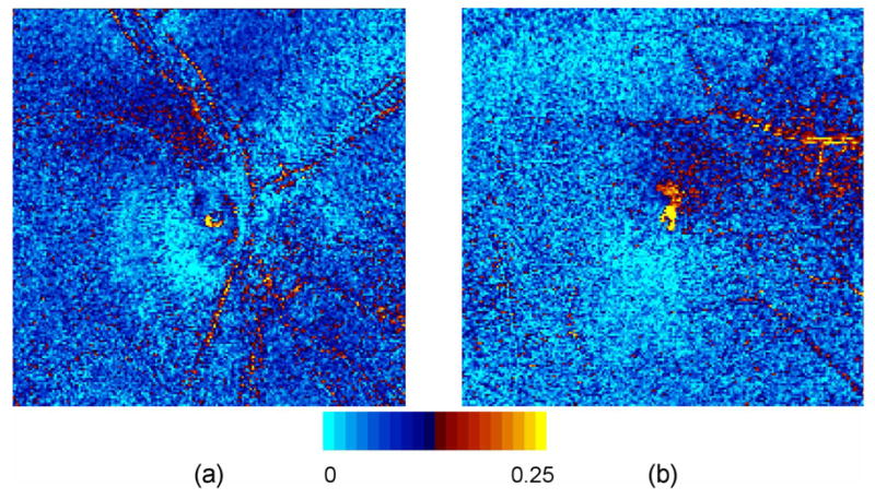
Frobenius error images for one subject. Yellow regions indicate an error greater than 0.25; mean error is approximately 0.1. (a): optic nerve head for right eye (for one subject); and (b): macula for right eye (for a different subject).

3.2 Anterior segment compensation

The anterior segment (AS), in particular the cornea, may exhibit retardance ranging from near zero to several times the retinal retardance [33,34]. This AS retardance component should be compensated in each dataset to obtain accurate retinal retardance images. This is done here by forming an estimate of the AS retardance, and then removing this retardance component using a Mueller matrix inverse algorithm. The estimation process is underdetermined, involving two “equations” (the measured retardance magnitude and orientation), and four unknowns (AS retardance magnitude and orientation and retinal retardance magnitude and orientation). The cornea may be modeled in general as a biaxial crystal with the fast axis normal to the surface [35]. Significant differences in the absolute magnitude and spatial variation of corneal birefringence have been observed among subjects [36]. Thus, the AS retardance component will have significant dependence on the location and incident angle of the probing beam, complicating the estimation process.

Two methods, “bowtie” and “screen”, have been described to estimate AS retardance from ocular polarization data. The experimental basis for the bowtie method was established by klein Brink and van Blokland [37]. Retardation images of a normal macula exhibit a distinct bowtie-shaped pattern. The bowtie method models the AS as a uniform linear retarder with fixed retardance magnitude and fixed axis, and the retinal Henle layer as a uniform linear retarder with fixed retardance magnitude and radial slow axis centered on the fovea. Where the axes are aligned, the overall retardance is a maximum equal to the sum, and where the axes are orthogonal the overall retardance is a minimum equal to the difference. The second harmonic of a Fourier series representing the intensity variation around a circle centered on the fovea provides an estimate of the constant AS retardance magnitude and orientation. The accuracy of bowtie method estimates is variable, depending on image quality and individual retardance variations in the macula region. The screen method suggested by Knighton and Huang [38] is an alternative, particularly when the bowtie pattern is weak or indeterminate. It is assumed that the AS retardance may be approximated by averages over a large area of the macula region (i.e. assumes macular retardance is negligible). Since the averaging area is larger, the effect of noise is reduced as compared to the bowtie method. Accuracy depends on the retardance variability in the nerve fiber layer, which may be significant.

After evaluating the bowtie and screen methods, we selected the screen method to perform AS compensation. To extract the estimated AS retardance magnitude δA and orientation φ_A from the Mueller matrix image, the original Mueller matrix M′ at each pixel is decomposed into component matrices for diattenuation (M′ _diatt), retardance (M′_ret), and depolarization (M′ _dep) using the Lu-Chipman algorithm. Retinal retardance matrices M_ret″ with AS component removed are calculated:

$${\mathbf{M}}_{\mathbf{ret}}^{″}={\left(LR\left[\frac{{\delta }_A}{2},{\phi }_A\right]\right)}^{-1}{\mathbf{M}}_{\mathbf{ret}}^{\prime }{\left(LR\left[\frac{{\delta }_A}{2},{\phi }_A\right]\right)}^{-1},$$ (8)

where LR[δ, φ] indicates a linear retarder with retardance δ and orientation φ. A new Mueller matrix is reassembled at each pixel as

$${\mathbf{M}}^{″}={\mathbf{M}}_{\mathbf{dep}}^{\prime }{\mathbf{M}}_{\mathbf{ret}}^{″}{\mathbf{M}}_{\mathbf{diatt}}^{\prime }.$$ (9)

The composite MM image assembled from the M″ matrices is then the full retinal polarization image with anterior segment retardance extracted.

Elsner has observed that retinal nerve fiber layer thickness and the related retardance magnitude are lowest and most uniform within a visual angle of about 1.25° radius from the fovea [39], implying that AS estimation would have best accuracy in this region. Our algorithm averages over a circular region within a 2.5° radius (5 pixel radius) of the fovea, irrespective of the bowtie appearance (back-reflection pixels were excluded). This method usually resulted in a uniform circularly symmetric (i.e. “donut-like”) residual foveal area retardance pattern after compensation (Fig. 5). The importance of corneal compensation is clearly illustrated in this figure, which shows that retardance is significantly over-estimated when compensation is not performed.

Fig. 5.

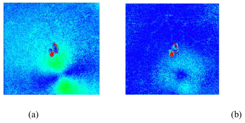
Anterior segment compensation using the “screen” method within a 2.5° radius of the fovea of a right eye. (a): uncompensated linear retardance image exhibits a bowtie pattern; (b) post-compensation linear retardance image exhibits a donut pattern. The spots in the center of the images are due to laser back-reflections within the instrument.

AS compensation was problematic for some datasets. In three cases our compensation method did not produce a circularly symmetric pattern near the fovea. Of the remaining 12 datasets, three had well defined donut-like patterns, and nine had irregular circular patterns. The wide variety of AS compensation results among these 15 normal subjects clearly illustrates the difficulty in reliably compensating the anterior segment. This is a shortcoming of the GDx-MM and similar retinal polarimeters, and might be mitigated for example through use of an independent means to estimate AS retardance [40].

3.3 Retinal polarization parameter images

Example polarization parameter images showing linear retardance, retardance orientation, diattenuation magnitude, diattenuation orientation, and depolarization index are shown in Fig. 6 for the ONH and in Fig. 7 for the macula. These images derive from the Mueller matrix images of Fig. 3, with use of the technique of Section 3.2 to perform corneal compensation.

Fig. 6.

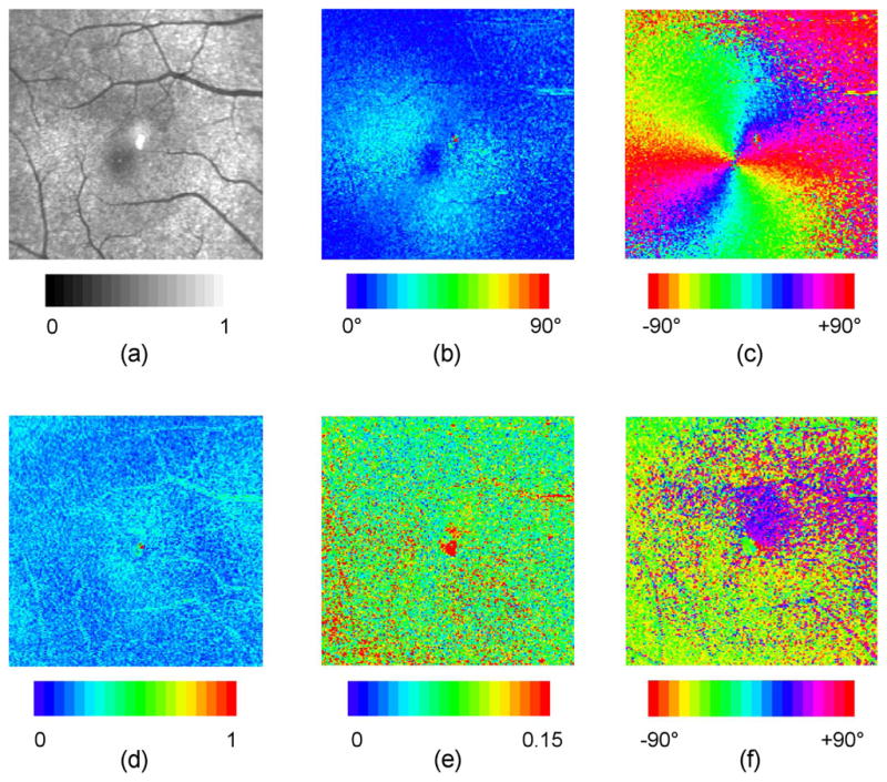
Polarization parameter images for ONH of right eye, for one subject. These images derive from the Mueller matrix image of Fig. 3(a), with use of the technique of Secion 3.2 to perform corneal compensation. (a): normalized average intensity; (b): linear retardance; (c): retardance orientation; (d): depolarization index; (e) diattenuation magnitude; (f) diattenuation orientation.

Fig. 7.

Polarization parameter images for macula of right eye, for one subject. These images derive from the Mueller matrix image of Fig. 3(b), with use of the technique of Secion 3.2 to perform corneal compensation. Details are the same as for Fig. 6.

A simple statistical analysis of our linear retardance, diattenuation, and depolarization index values was performed over full images for each of the 15 subjects. This analysis is intended to facilitate comparison to previously reported results, and to illustrate the typical range of values seen. Pixels with high Frobenius error were excluded from the calculations. Table 3 tabulates lowest and highest values from each image-averaged parameter, along with the mean and standard deviation of the distributions of individual pixel values over the fifteen images.

Table 3.

Polarization parameter statistical summary

Parameter	Minimum	Maximum	Mean, Std Dev
ONH linear retardance	23.3º	34.9º	28.4º ± 15.5º
Macula linear retardance	9.2º	21.1º	17.3º ± 9.4º
ONH diattenuation magnitude	0.07	0.11	0.09 ± 0.05
Macula diattenuation magnitude	0.07	0.10	0.08 ± 0.05
ONH depolarization index	0.21	0.29	0.25 ± 0.07
Macula depolarization index	0.21	0.32	0.25 ± 0.07

Linear retardance images of the ONH show highest magnitude in superior and inferior locations (particularly near large vessels) and lowest magnitude in nasal and temporal regions. These findings are consistent with the typical thickness variation of a normal retinal nerve fiber layer. The mean retardance averaged over the 15 subjects is 28.4º ± 15.5º for ONH and 17.3º ± 9.4º for macula. The variation around the ONH was approximately 10° to 60°, consistent with the results of Huang et al. (mean retardance of 33 ± 3°, variation from 10° to 50°) [41]. Retardance orientation images show a fast axis orientation that is horizontal at 12 and 6 o’clock, and vertical at 3 and 9 o’clock, with smooth variation between. The fast axis thus exhibits approximate circular symmetry about a center point (the fovea or the ONH), and the slow axis is radially symmetric about this center point, as would be expected given the radial orientation of the retinal fibers in these areas. The “pinwheel” patterns in the macula region are consistently well defined and symmetric over the 15 datasets. The patterns about the ONH exhibit lower symmetry, as the fibers in this area are not as precisely radial as the Henle fibers in the macula.

Depolarization index images show weak features with mean value of approximately 25%, indicating for polarized light incident, the average degree of polarization is 75%. Higher depolarization of up to 40% is seen particularly in annular regions around the ONH and in localized regions near the macula. Depolarization along major blood vessels is higher than in surrounding regions; this may be due to higher scattering from vessels, but may also be a result of lower accuracy due to the lower signal to noise ratio. These results are in reasonable agreement with degree of polarization measurements by van Blokland and Norren (80%–90%) [42] and Bueno (67% – 92%) [9]. Localized higher depolarization in the macula has also been observed by Elsner [43].

Diattenuation magnitude images show weak features and exhibit mean value of approximately 8%, in reasonable agreement with measurements by Park et al (6%) [44], Kemp et al (2%) [12], and Bueno and Artal (10%) [26]. Diattenuation magnitude is consistently higher superior and inferior to the ONH, but with qualitatively somewhat different appearance from retardance magnitude, suggesting that the diattenuation profile may be partly but not completely due to the arrangement of fibers in the nerve fiber layer. The diattenuation orientation images (though noisy due to low diattenuation magnitude) are qualitatively similar to the retardance orientation images, also suggesting a significant contribution from the nerve fiber layer. These results are in general agreement with models [12,45] which predict that the structural arrangement of fibers in the nerve fiber layer should give rise to dichroism (and hence diattenuation) as well as birefringence. Bueno and Artal observed no correlation between ocular retardance and diattenuation axes using a nonimaging Mueller matrix polarimeter [26], but as no corneal compensation was performed the birefringence axis measurement was dependent on both retinal and corneal contributions. Diattenuation magnitude images for the macula region show variation about the fovea, which is most likely due to Henle layer variations. The orientation images are variable among subjects, showing either no preferred orientation, localized regions of preferred orientation as in Fig. 7, or a single preferred orientation. The measured diattenuation necessarily includes contributions from both anterior segment and retina. Bueno and Jaronski measured single-pass diattenuation of 0.03±0.01 in bovine and porcine corneas [19], less than but comparable to the diattenuation reported here. For accurate retinal diattenuation measurement anterior segment diattenuation may need to be compensated using an analog to the retardance technique discussed in Section 3.2.

To compare GDx-MM and GDx measurements of linear retardance (the GDx is demonstrably less accurate due to depolarization and diattenuation coupling into the linear retardance measurement), data was collected at Indiana University on three study subjects using a GDx. Raw image sets were processed to produce retardance values according to the algorithm in [38]. To avoid ambiguities from the different AS compensation methods, GDx-MM post-processing compensation was not performed and the corneal compensator retarder was removed from the GDx. The data from the two instruments were similar (Fig. 8), but the retardance measured with the GDx-MM was consistently higher. For the ONH shown in Fig. 8, linear retardance measured using the GDx-MM was δ_M = 48.1° ± 16.8°, depolarization index using the GDx-MM was a = 0.21 ± 0.06, and linear retardance using the GDx over approximately the same retinal field of view was δ_G = 39.3° ± 16.9°. By modeling the nerve fiber layer as an ideal linear retarder of retardance δ_M combined with a pure depolarizer which imparts a degree of polarization (1–a) to all states, the approximate expected GDx error in retardance measurement may be calculated [25]. For the data of Fig. 8 the calculated error is 12°, in good agreement with the observed error of δ_M − δ_G ≈ 9°. Our results compare favorably with the error of approximately 10° measured by Bueno in an eye with a ≈ 0.2 [9].

Fig. 8.

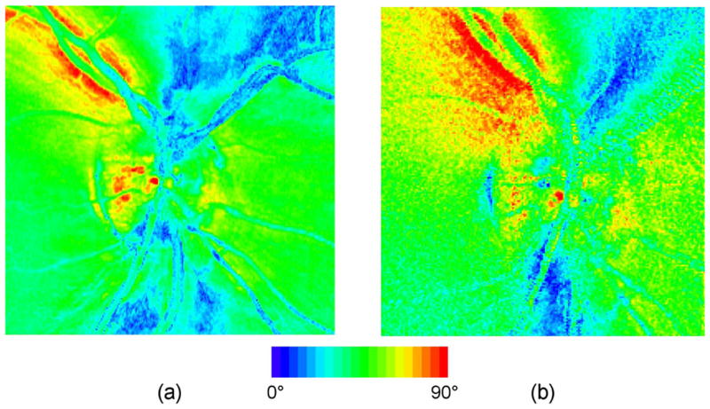
Comparison of uncompensated linear retardance measurement for the right eye of same subject with (a) GDx and (b) GDx-MM.

4. Conclusions

A complete imaging retinal polarimeter, the GDx-MM, has been designed, optimized, calibrated, validated, and used in a clinical setting to obtain retinal data for normal human subjects. Images showing the spatial variation of polarization parameters were generated and analyzed. Collected data was demonstrated to be consistent with previously reported results. Space limitations within the GDx mandated the use of non optimal polarization components, liquid crystal variable retarders, which limited the polarization accuracy of the instrument.

No subjects with retinal disease were evaluated for this study; however, it is important to consider how each polarization parameter image might provide useful information in disease diagnosis and monitoring. Conjectures can be made based on the demonstrated utility of similar instruments such as the Carl Zeiss Meditec GDx and knowledge of polarization effects in the eye. Retardance images may provide insight into the Henle layer, retinal nerve fiber layer, cornea, and lens. The most apparent use is in monitoring the thickness of the nerve fiber and Henle layers, as an indicator of the presence and progression of glaucoma. Disruptions in or absence of the bowtie in the uncompensated linear retardance plot and/or the pinwheel in the retardance orientation plot may indicate disruptions of the Henle layer.

Based on qualitative comparisons of the 15 datasets, diattenuation orientation and retardance orientation have similar appearance in the ONH, suggesting that much of the diattenuation arises from the nerve fiber layer. The diattenuation has a higher spatial frequency component than the retardance and so may be simultaneously indicating the configuration of other retinal tissues. These results suggest that retinal diattenuation measurements may be used to probe the nerve fiber layer structure with significantly lower anterior segment effect than is observed in the retardance measurement. This hypothesis is supported by a study by Naoun et al. [46] in which significant differences in dichroism were observed between normal and glaucomatous eyes. Huang and Knighton [11] have modeled the nerve fiber layer fibrils as an array of cylinders. They predict a thickness-independent diattenuation with magnitude similar to our observations, but with orientation that is parallel to the fibrils at normal incidence, in contradiction to our observations (Fig. 6(f)). Our results may derive from deeper back-scattering events, in which case diattenuation magnitude would be thickness dependent. The GDx-MM, with its unique ability to measure a full Mueller matrix in direct backscatter, is well suited to explore the validity of the hypotheses set forth in scientific models.

Depolarization images are of ongoing interest since they emphasize multiple scattering and deeper scattering structures [5–9]. Elsner and colleagues have generated depolarization images by reprocessing GDx data to find the minimum intensity in the cross polarized channel. This metric, while not an exact calculation of the depolarization index, responds strongly to depolarization and weakly to elliptical retardance, elliptical diattenuation, and inhomogeneous (non aligned) linear retardance and diattenuation. By this method Elsner observed that many disease-related features have higher contrast in the depolarization image, including drusen, pools of fluid and leakage points, vessel abnormalities, edema, exudative lesions, peripapillary hyperpigmentation, and neovascular membranes. Naoun et al. have measured significant differences in degree of polarization between normal and glaucomatous eyes, attributed to the loss of ganglion cells and axons [46]. It is thus reasonable to predict that depolarization images would facilitate detection and monitoring of disease processes which disrupt the regular structure of retinal tissue.