Ab initio protein modeling into cryoEM density maps using EM-Fold

Abstract

EM-Fold was used to build models for nine proteins in the maps of GroEL (7.7 Å resolution) and ribosome (6.4 Å resolution) in the ab initio modeling category of the 2010 cryoEM modeling challenge. EM-Fold assembles predicted secondary structure elements (SSEs) into regions of the density map that were identified to correspond to either α-helices or β-strands. The assembly uses a Monte Carlo algorithm where loop closure, density-SSE length agreement, and strength of connecting density between SSEs are evaluated. Top scoring models are refined by translating, rotating and bending SSEs to yield better agreement with the density map. EM-Fold produces models that contain backbone atoms within secondary structure elements only. The RMSD values of the models with respect to native range from 2.4 Å to 3.5 Å for six of the nine proteins. EM-Fold failed to predict the correct topology in three cases. Subsequently Rosetta was used to build loops and side chains for the very best scoring models after EM-Fold refinement. The refinement within Rosetta’s force field is driven by a density agreement score that calculates a cross correlation between a density map simulated from the model and the experimental density map. All-atom RMSDs as low as 3.4 Å are achieved in favorable cases. Values above 10.0 Å are observed for two proteins with low overall content of secondary structure and hence particularly complex loop modeling problems. RMSDs over residues in secondary structure elements range from 2.5 Å to 4.8 Å.

Introduction

Cryo-electron microscopy (cryoEM) has become the protein structure elucidation method of choice for proteins that evade crystallization and are too large for nuclear magnetic resonance (NMR). It is particularly well suited for large proteins or protein complexes. Within the last few years the first cryoEM density maps at resolutions better than 4 Å have been published^1,2. Density maps in this resolution range allow direct protein model building by tracing the backbone. However, the vast majority of published cryoEM density maps still fall in the medium resolution (4 – 10 Å resolution) or low resolution (worse than 10 Å resolution) category. Over the past 20 years researchers have developed a plethora of computational methods and algorithms that aid in the interpretation of these medium to low resolution density maps. A comprehensive overview of these methods can be found in³. In summary, the available methods can be grouped into the following categories: A) methods that segment a density map of a protein complex into parts that correspond to density of individual proteins. These programs are applicable to both medium and low resolution density maps. B) Methods that identify secondary structure elements in a density map. This is generally only possible for medium resolution density maps as α-helices become visible at about 10 Å resolution and β-strands can be discerned at about 5 Å resolution. C) Methods that fit high resolution protein models (generally crystal structures) into a density map. These methods are referred to as rigid body fitting algorithms as they probe different positions and orientations of high resolution models in density maps without altering the fitted structure. D) Methods that fit high resolution protein models (generally crystal structures) into a density map while simultaneously adapting the fitted structure to obtain the best possible agreement between structure and density map. These methods are referred to as flexible fitting algorithms. Methods in categories C and D can generally be applied to medium and low resolution density maps. E) A last group of programs aims to “de novo” or “ab initio” fold proteins from their primary sequence using the density map as a folding restraint. Methods in this category generally work best with medium and high resolution density maps.

EM-Fold, a member of group E, was developed to use medium resolution cryoEM density maps as folding constraints for de novo protein folding⁴. It assumes that secondary structure elements (SSEs) are identified in the map. Using the primary sequence of the protein, EM-Fold builds up a pool of predicted SSEs from a consensus of several secondary structure prediction methods. Predicted secondary structure elements are then assembled into the density segments identified to correspond to SSEs. A refinement step where SSEs are translated, rotated and bent to optimize SSE packing and agreement with the density map is followed by loop building and iterative relaxation and refinement in Rosetta. EM-Fold has previously been tested in two benchmarks on a total of 37 proteins of known structure⁴. In both tests, EM-Fold was able to build the correct topology among the top scoring proteins in about 70% of the cases. The improved version in combination with Rosetta⁵ was also able to refine the majority of the benchmark proteins to atomic resolution ¹⁵. The vast majority of benchmark cases so far had simulated density maps.

The cryoEM modeling challenge held in 2010 offered an avenue to test algorithms using experimental density maps on problems falling into the five described categories. A sixth category tested the model building from high resolution density map through backbone tracing. Experimental density maps from six different biological systems at different resolutions were provided. The resolutions of the maps ranged from 3.0 Å to 23.5 Å. Three of the provided maps were high resolution, nine were medium resolution and one map was low resolution. In the context of the cryoEM modeling challenge EM-Fold was tested on a total of nine proteins extracted from two of the provided density maps. These nine proteins were chosen because their maps were medium resolution, SSEs were visible in the maps, the respective protein size did not exceed previously tested sizes for EM-Fold and the SSE content was at least 35%. Here we present the results of using EM-Fold to build models for these nine proteins.

Results and Discussion

EM-Fold is a program that folds proteins de novo into medium resolution density maps. For this only the primary sequence and positions of identified secondary structure elements from the density map are used. Based on the primary sequence, secondary structure elements are predicted on stored in a pool of SSEs. In the initial assembly step, SSEs from the pool are randomly placed in the density map to build sets of possible protein models. Models are scored based on their SSE-density rod length agreement and their loop properties. A subsequent EM-Fold refinement step slightly perturbs the SSEs to maximize agreement with the shapes of the observed density rods. The final step is a multi-step refinement protocol in Rosetta that builds loop regions and improves the protein models. EM-Fold was used to predict structures of nine proteins based on their density map in the ab initio modeling category of the modeling challenge.

Challenge proteins have lower secondary structure content than EM-Fold benchmark^4,15

Experimentally determined density maps of six different macromolecular complexes were provided in the modeling challenge. These maps contained a total of 116 distinct chains. Nine proteins (2C7DU, 3FICD, 3FICG, 3FICZ, 3FINF, 3FING, 3FINL, 3FINR, 3FINU) from two different maps (GroEL at 7.7 Å resolution and ribosome at 6.4 Å resolution) were picked as targets for EM-Fold de novo protein folding. Selection criteria included the resolution of the map (around 7 Å), overall quality of the map (SSEs had to be visible), and protein size (EM-Fold has been tested for proteins up to 350 amino acids and up to 15 SSEs). The high computational demand of the protocol made it prohibitive to work on all 19 remaining test cases. In turn we focused on smaller proteins with a predicted secondary structure content of at least 35% - i.e. cases that we expect are favorable for EM-Fold. Crystal structures were available for all target proteins and results were evaluated based on comparison with the PDB coordinates. Table 1 displays the size, number of SSEs, and fold complexity as measured by relative contact⁶ order for all test proteins. Contact order is defined as the average sequence separation of all pairs of residues that are in contact, i.e. that are within a certain distance in the folded protein. High contact orders indicate complex protein fold topologies as there are many non-local contacts in the protein and represent a formidable challenge to computational protein folding. These numbers are in approximate agreement with the proteins used in the previously published benchmarks of EM-Fold^4,15. Relative contact orders range from 0.03 to about 0.15, with an average of 0.08 and a standard deviation of 0.03 (see Figure 1). Proteins within both groups scatter over the full range. Differences become apparent when comparing the secondary structure content of the challenge proteins with those from previous benchmarks. The secondary structure content of the proteins targeted in the challenge ranges from 36% to 63% (with an average of 50%) which is considerable less than the 68% average SSE content in the previous benchmarks. As a result of this loop regions in challenge proteins were considerably longer than for the benchmark proteins. This situation complicates two parts of the EM-Fold protocol: The EM-Fold assembly step relies on a loop score that ensures SSEs can still be connected once placed into the density. Longer loops will increase the total number of possible SSE placements that need to be sampled as consistent with this score. Secondly, the last step of model construction incorporates loop regions and refines the atomic-detail model using the density map as a restraint. This part of EM-Fold has to sample larger conformational spaces for the long loop regions.

Table 1.

Summary of structural properties of the nine modeling challenge target proteins of EM-Fold.

protein	# residues	# helices/# strands [a]	Contact order [b]	Secondary structure content (total, helical, strand) [%] [c]
2C7DU	97	0/4	0.145	37, 3, 34
3FICD	208	5/0	0.062	45, 37, 8
3FICG	155	6/0	0.065	55, 52, 3
3FICZ	405	6/15	0.063	55, 21, 34
3FINF	208	4/1	0.074	40, 32, 8
3FING	181	4/2	0.099	36, 25, 11
3FINL	138	4/3	0.067	59, 41, 18
3FINR	117	4/2	0.085	56, 44, 12
3FINU	117	4/0	0.036	63, 63, 0
Average contact order and standard deviation			0.077 (0.031)

^[a]The number of α-helices and β-strands with at least 12 and 5 residues respectively is given.

^[b]Relative contact orders were computed with a contact cutoff of 6 Å.

^[c]The relative amount of secondary structure elements (α-helices and β-strands) of the entire sequence is listed.

Figure 1.

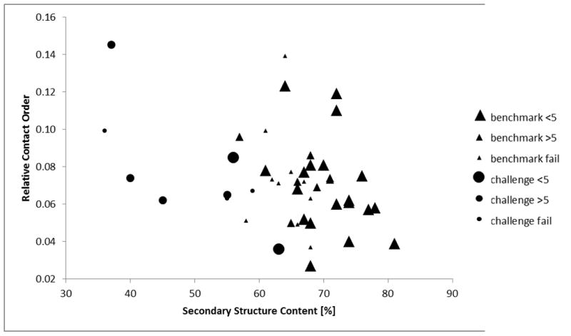
Comparison of contact order and secondary structure content of proteins targeted in the modeling challenge and of proteins from previous benchmarks. Relative contact order with a contact cutoff of 6 Å is plotted against total secondary structure content in percent (sum of helical and strand content). The nine proteins that were modeled with EM-Fold in the challenge are marked with circles, while proteins from previous EM-Fold benchmarks are plotted using triangles. The size of the symbols correlates with the success in folding the protein. The largest symbols correspond to cases where full length models with an RMSD of less than 5 Å were generated. Medium sized symbols correspond to cases where building the model was still possible, but the RMSD was worse than 5 Å. Small symbols indicated failure to build a model having the correct topology. Challenge proteins exhibit a lower SSE content than proteins from previous benchmarks.

Assembly step identifies correct topology for six out of nine challenge proteins

Besides secondary structure prediction identification of density rods corresponding to secondary structure elements is a crucial prerequisite for execution of EM-Fold. As both the segmentation of density maps and the automated identification of SSEs in the density maps were addressed by separate categories of the modeling challenge we decided to use information from the crystal structures to perform these tasks to not bias EM-Fold input. The first step of the EM-Fold folding protocol identified the correct topology for six out of nine proteins targeted in the challenge. This corresponds to a success rate of about 67% and is comparable to the ca. 70% success rate seen in previous benchmarks. The 67% success rate encompasses the success of correctly predicting secondary structure elements and assembling models with the correct topology in the EM-Fold assembly step. This suggests that the loop score also works reliably in distinguishing correct from incorrect topologies in the context of longer loop lengths. The RMSDs of the models after the assembly step range from 2.6 Å to 5.3 Å. Table 2 summarizes the results of the assembly step. Models for the successful topologies were advanced to the refinement step where SSEs are translated, rotated and bent to maximize the agreement of the model with the experimental density map. The EM-Fold refinement step improves the RMSDs of the models to fall in a range between 2.4 Å and 3.5 Å. Column 3 in Table 2 lists all the results of the refinement step. The quality of the models after refinement step is comparable in terms of RMSD to refined models in previous benchmarks^4,15.

Table 2.

Summary of folding results for the nine modeling challenge target proteins of EM-Fold.

protein	RMSD [Å] [a]
	EM-Fold assembly	EM-Fold refinement	Rosetta refinement
2C7DU	(2.6 Å)	(2.4 Å)	5.6 Å (2.5 Å)
3FICD	(3.8 Å)	(3.1 Å)	11.4 Å (4.8 Å)
3FICG	(5.3 Å)	(3.5 Å)	7.0 Å (3.6 Å)
3FICZ	-	-	-
3FINF	(3.0 Å)	(2.8 Å)	13.9 Å (3.5 Å)
3FING	-	-	-
3FINL	-	-	-
3FINR	(4.2 Å)	(2.4 Å)	4.6 Å (3.7 Å)
3FINU	(4.3 Å)	(3.3 Å)	3.4 Å (2.6 Å)

^[a]RMSDs are calculated over all backbone atoms. RMSDs over SSE residues are in parentheses. Models after the EM-Fold assembly and refinement step don’t contain residues in loop regions.

Full length model accuracy is limited by long loop lengths

Starting from models after the EM-Fold refinement step (RMSDs between 2.4 Å and 3.5 Å) it was hypothesized that the some of the six successful topologies can be refined to atomic detail accuracy by Rosetta⁵. However, none of the proteins was refined below an RMSD of 3 Å. The correct topology models after Rosetta refinement range from 3.4 Å to 13.9 Å RMSD. When calculating the RMSD over just the residues in secondary structure elements, the RMSDs are considerably better (2.5 Å to 4.8 Å RMSD). In some cases these values are slightly worse than the starting models after the EM-Fold refinement step. This can be attributed to the necessity of having to move residues in SSEs in order to construct the long loop regions. Results after Rosetta refinement are shown in Table 2. Superimpositions of the final models with the experimental structures and the density maps are also shown in Figure 2, Figure 3 and Figure 4. It can be seen that the large RMSD values result from deviations in the loop regions. It has been shown that building longer loops is a considerable more challenging task in Rosetta than building shorter loops⁷. These results reveal a limitation of the EM-Fold model building protocol that was not apparent in previous benchmarks. Building of low RMSD full atom models heavily depends not only on low RMSDs of EM-Fold refined models but also on high sequence coverage of secondary structure elements in the SSE pool. Figure 2 and Figure 3 also display the Rosetta energy versus SSE RMSD plots over the three rounds of refinement. These plots highlight one of the most challenging tasks that is associated with evaluation of the models that emerge from the EM-Fold protocol – identification of the correct topology if the native structure was not known. While the correct topology is not a member of the lowest energy cluster in all cases, it should be noted that it is within one of the lowest scoring clusters in all proteins throughout all three rounds of refinement. This demonstrates the ability of the Rosetta scoring function to identify native-like topologies even in the absence of atomic-detail information. Previous benchmarks demonstrated that it is possible to uniquely identify a native-like model using the Rosetta score if the RMSD values fall below a certain threshold. Unfortunately this was not possible in these cases – probably due to the smaller secondary structure content of the proteins. However the correct topology is still identified as one of the top 10 scoring model. This gives researchers the ability to experimentally test a small number of hypothetical structures. Figure 5 presents models from rounds 1–3 for 3FINU, the protein that was most accurately predicted using EM-Fold. The biggest challenge in this case was the long, bent central helix. Every step of the protocol was able to improve the model matching the experimental structure and in particular the bent helix more closely.

Figure 2.

Superimposition of final models after Rosetta refinement with native structures from pdb files. Examples for models with good overall agreement are shown. Superimposition of the final models (colored in rainbow) of 2C7DU (A), 3FINR (B) and 3FINU (C) with the original PDB structures (grey) are shown. Additionally, plots of Rosetta full atom energy vs RMSD of the model SSEs with respect to the native structure are shown. Structures from the first round of refinement are colored green, structures from the second round are blue while the structures after the third round are shown in black. RMSDs are calculated over all backbone atoms. (A) 2C7DU has 97 residues. The model shown has a RMSD of 5.6 Å over the full length of the protein and 2.5 Å over the residues in SSEs. (B) 3FINR has 117 residues. The model shown has a RMSD of 4.6 Å over the full length of the protein and 3.7 Å over the residues in secondary structure elements. (C) 3FINU has 117 residues. The model shown has a RMSD of 3.4 Å over the full length of the protein and 2.6 Å over the residues in secondary structure elements.

Figure 3.

Superimposition of final models after Rosetta refinement with native structures from pdb files. Examples for models are shown that exhibit large RMSD over the full length of the model, but are in good agreement in regions of secondary structure. Superimposition of the final models (colored in rainbow) of 3FINF (A) and 3FICD (B) with the original PDB structures (grey) are shown. Additionally, plots of Rosetta full atom energy vs RMSD of the model SSEs with respect to the native structure are shown. Structures from the first round of refinement are colored green, structures from the second round are blue while the structures after the third round are shown in black. RMSDs are calculated over all backbone atoms. (A) 3FINF has 208 residues. The model shown has a RMSD of 13.9 Å over the full length of the protein and 3.5 Å over the residues in SSEs. (B) 3FICD has 208 residues. The model shown has a RMSD of 11.4 Å over the full length of the protein and 4.8 Å over the residues in secondary structure elements.

Figure 4.

Superimposition of the final models after Rosetta refinement with native structures from pdb files and experimental density maps. Superimposition of the final models (colored in rainbow) of 2C7DU (A), 3FINR (B), 3FINU (C), 3FINF (D) and 3FICD (E) with the original PDB structures (grey) are shown.

Figure 5.

Evolution of 3FINU models over the steps of the modeling protocol. Superimposition of the correct topology models (colored in rainbow) of 3FINU after the EM-Fold assembly step (A), after the EM-Fold refinement step (B) and the Rosetta refinement (C, D) are shown. The original PDB structures (grey) are shown for comparison. (A) The model after the EM-Fold assembly step only contains residues in SSEs and has an RMSD of 4.3 Å to the native structure. (B) The EM-Fold refinement improves the model to an RMSD of 3.3 Å. (C) Rosetta refinement finally builds in missing loop regions and refines the model to an RMSD of 3.4 Å over the full length of the protein and 2.6 Å over residues in SSEs. Panel D shows the final model after Rosetta refinement within the experimental ribosome density.

Lessons from the challenge

EM-Fold has been successful to predict the correct topology for six out of nine test cases from the cryoEM modeling challenge de novo. This result matches performance in previously published benchmarks^4,15. Nevertheless, the experiment provided interesting insights that will help to improve the method in the future: 1) Large loop regions proved problematic in building high accuracy full length models of the proteins. A stepwise loop construction using the density as a restraint is one possible avenue to address this limitation. 2) It became apparent that EM-Fold performs best for proteins with high secondary structure content. While not unexpected this finding highlights a limitation of the method. 3) When using EM-Fold in the challenge it was assumed that the density map had already been segmented to reveal the protein chain of interest and that SSEs had been identified from the density map. Algorithms that perform these tasks are available and were tested during the challenge as well. In the challenge EM-Fold integrated Rosetta for atomic-detail refinement⁵. Thus, EM-Fold should be regarded as one algorithm in a set of many valuable tools that can be part of protein modeling from cryo-EM density maps.

Being able to test EM-Fold on a large number of experimental maps for a variety of different systems gave a clearer picture of the strengths and weaknesses of the algorithm. Possible avenues of improvement include increasing the accuracy of models after EM-Fold refinement simplifying and accelerating the atomic-detail refinement step. Stepwise construction of loop regions, inclusion of shorter secondary structure elements, or a sequence shift move will be tested in this regard. In the scoring function sequence-dependent terms will be added that discriminate better for native-like placement of SSEs in the assembly phase.

We do believe that this challenge benefitted the still young field of cryoEM modeling techniques and will spur many improvements of the involved methods. The large collection of experimental density maps gathered made for an impressive benchmark set. The challenge not being blind is a limitation but not a critical one. Many of the computational methods for density map modeling (ours included) are still in early stages compared to modeling techniques for more established methods like X-ray crystallography and NMR spectroscopy. The challenge provided feedback and some comparison between methods. It would be advantageous if future challenges had some element to blind-prediction. We would like to thank the organizers for their hard work in putting the challenge together.

Materials and Methods

Folding protocol

The general EM-Fold folding protocol is described in⁴. EM-Fold had previously been used to predict models for 37 soluble proteins based on simulated density maps. There EM-Fold had been demonstrated to work well for proteins ranging in size between 150 and 350 amino acids. The scenario encountered in the challenge was slightly different from the benchmark situation in that the maps did not contain a single protein but in most cases multiple copies of several different proteins. Before running EM-Fold it is necessary to identify and segment density belonging to a single protein chain and subsequently identify secondary structure elements in the segmented density. Both of these steps were addressed in separate categories in the challenge: “Protein Segmentation” and “Secondary Structure Annotation”. We thus decided to simply assume that algorithms exist to perform these tasks and segmented the density map based on information from the crystal structure. Our contribution was testing the core capabilities of EM-Fold in the ab initio modeling category. For the challenge prediction the secondary structure prediction algorithms jufo^8,9, psipred¹⁰ and PROFphd^11–13 were used. The individual predictions and a consensus of the three methods were inserted in a pool of secondary structure predictions. Based on these predicted SSEs, the assembly step placed SSEs into the density map. A dynamic resizing of secondary structure elements accompanied by scoring the model secondary structure agreement with the original predictions was applied during the assembly step. As demonstrated in previous benchmarks the assembly step is not able to identify the correct topology uniquely by score alone. Thus the top 150 scoring topologies after the assembly step are used as input for the refinement step. If the correct topology does not score among the top 150 models the protein is labeled a failure. The refinement step rotated, translated and bent SSEs. The agreement of the refined model with the density map was judged by a cross correlation density agreement score. The models generated with the refinement step do not contain residues in loop region or side chain coordinates. The top 75 scoring topologies after the refinement step are used as input for the Rosetta loop building and refinement. Three iterative rounds of Rosetta⁵ refinement were used to build loops and side chains and refine the full atom models further.

EM-Fold parameters

This section provides sample commandlines for the EM-Fold assembly and refinement steps and discusses important parameters. A sample commandline for the assembly step is:

bcl.exe Fold -protocols EM -nmodels 1 -fasta protein.fasta -pool protein.pool -mc_number_iterations 2000 500 -mc_temperature_fraction 0.25 0.05 -body_restraint protein. cst_body 3.5 3.5 4.8 4.8–1.0-print_body_assignment -score_density_connectivity protein.mrc -write_minimization improved -sspred JUFO PSIPRED PROFphd -sspred_path_sspred_files/

2000 rejected Monte Carlo steps are chosen as the terminate criterion (also 500 rejected steps in a row cause early termination). The target percentage of accepted steps falls from 25% at the beginning of the simulation to 5% at the end of the simulation. A symmetric energy well of depth -1.0 and width 3.5 Å (fall-off to depth 0.0 at deviations of 4.8 Å and beyond) is chosen. A sample commandline for the refinement step is:

bcl.exe Fold -protocols EM -nmodels 1 -native protein.pdb -start_model assembly_model.pdb -score_density_agreement protein.mrc 7.7 TrilinearInterpolation CCC -fasta protein.fasta -pool protein.pool -mc_number_iterations 2000 400 -mc_temperature_fraction 0.25 0.05 -em_refinement

2000 rejected Monte Carlo steps are chosen as the terminate criterion (here already 400 rejected steps in a row cause early termination). The target percentage of accepted steps falls from 25% at the beginning of the simulation to 5% at the end of the simulation. The resolution of the simulated map for cross correlation calculation should ideally be identical to the resolution of the experimental map (7.7 Å in the sample commandline). These parameters were used for all the proteins in the challenge and the wide variety of benchmark systems and there should be no need to dramatically adjust them. Most notably the size of the energy well for the length agreement score may have to be adjusted according to the precision of the predicted secondary structure elements.

Nine protein testcases

Nine distinct proteins (chain U from 2C7D, chain D from 3FIC, chain G from 3FIC, chain Z from 3FIC, chain F from 3FIN, chain G from 3FING, chain L from 3FIN, chain R from 3FIN, chain U from 3FIN) from two different medium resolution maps (GroEL at 7.7 Å resolution and ribosome at 6.4 Å resolution) were picked as targets for EM-Fold de novo protein folding. The protein sizes ranged from 97 to 405 residues. In its newest version EM-Fold can deal with both α-helices and β-strands. Three of the proteins were α-proteins, one was a pure β-protein and the remaining five proteins were α/β-proteins. A detailed summary of the protein structural statistics can be found in Table 1. Contact orders were calculated using the contact order server at the University of Washington¹⁴.

References

- 1.Zhou ZH. Curr Opin Struct Biol. 2008;18:218–228. doi: 10.1016/j.sbi.2008.03.004. [DOI] [PMC free article] [PubMed] [Google Scholar]
- 2.Liu H, Jin L, Koh SB, Atanasov I, Schein S, Wu L, Zhou ZH. Science. 2010;329:1038–1043. doi: 10.1126/science.1187433. [DOI] [PMC free article] [PubMed] [Google Scholar]
- 3.Lindert S, Stewart PL, Meiler J. Curr Opin Struct Biol. 2009;19:218–225. doi: 10.1016/j.sbi.2009.02.010. [DOI] [PMC free article] [PubMed] [Google Scholar]
- 4.Lindert S, Staritzbichler R, Wotzel N, Karakas M, Stewart PL, Meiler J. Structure. 2009;17:990–1003. doi: 10.1016/j.str.2009.06.001. [DOI] [PMC free article] [PubMed] [Google Scholar]
- 5.DiMaio F, Tyka MD, Baker ML, Chiu W, Baker D. J Mol Biol. 2009;392:181–190. doi: 10.1016/j.jmb.2009.07.008. [DOI] [PMC free article] [PubMed] [Google Scholar]
- 6.Bonneau R, Ruczinski I, Tsai J, Baker D. ProteinSci. 2002;11:1937–1944. doi: 10.1110/ps.3790102. [DOI] [PMC free article] [PubMed] [Google Scholar]
- 7.Rohl CA, Strauss CE, Chivian D, Baker D. Proteins. 2004;55:656–677. doi: 10.1002/prot.10629. [DOI] [PubMed] [Google Scholar]
- 8.Meiler J, Baker D. Proc Natl Acad Sci U S A. 2003;100:12105–12110. doi: 10.1073/pnas.1831973100. [DOI] [PMC free article] [PubMed] [Google Scholar]
- 9.Meiler J, Muller M, Zeidler A, Schmaschke F. J Mol Model. 2001;7:360–369. [Google Scholar]
- 10.Jones DT. Journal of Molecular Biology. 1999;292:195–202. doi: 10.1006/jmbi.1999.3091. [DOI] [PubMed] [Google Scholar]
- 11.Rost B, Sander C. Proteins. 1994;19:55–72. doi: 10.1002/prot.340190108. [DOI] [PubMed] [Google Scholar]
- 12.Rost B, Sander C. Journal of Molecular Biology. 1993;232:584–599. doi: 10.1006/jmbi.1993.1413. [DOI] [PubMed] [Google Scholar]
- 13.Rost B, Sander C. Proceedings of the National Academy of Sciences. 1993;90:7558–7562. doi: 10.1073/pnas.90.16.7558. [DOI] [PMC free article] [PubMed] [Google Scholar]
- 14.Plaxco KW, Simons KT, Baker D. Journal of Molecular Biology. 1998;277:985–994. doi: 10.1006/jmbi.1998.1645. [DOI] [PubMed] [Google Scholar]
- 15.Lindert S, Alexander N, Wotzel N, Karakas M, Stewart PL, Meiler J. EM-Fold: De Novo Atomic-Detail Protein Structure Determination from Medium-Resolution Density Maps. Structure. 2012;20:464–478. doi: 10.1016/j.str.2012.01.023. [DOI] [PMC free article] [PubMed] [Google Scholar]