Dependence of global temperatures on atmospheric CO₂ and solar irradiance

Abstract

Changes in global average temperatures and of the seasonal cycle are strongly coupled to the concentration of atmospheric CO₂. I estimate transfer functions from changes in atmospheric CO₂ and from changes in solar irradiance to hemispheric temperatures that have been corrected for the effects of precession. They show that changes from CO₂ over the last century are about three times larger than those from changes in solar irradiance. The increase in global average temperature during the last century is at least 20 times the SD of the residual temperature series left when the effects of CO₂ and changes in solar irradiance are subtracted.

Although it is generally conceded that the average surface temperature of the Earth has increased by about 0.6°C during the last century, there is little agreement on the cause of this warming. The primary cause of this disagreement is uncertainty about the relative contribution to this warming of atmospheric CO₂ and changes in solar irradiance. The purpose of this paper is to describe some data analysis that may help to discriminate between solar and CO₂ effects, and to give estimates of the relative magnitudes of these two effects. The difference between analysis such as those described in ref. 1 and those here is that this data analysis is based on deseasonalized temperature time series where the effects of precession were included.* The detection of precession in instrumental temperature series and the necessity of including it when removing the annual cycle from temperature data was demonstrated in ref. 2. I also describe some of the statistical peculiarities and limitations of these data series and suggest where better data are needed.

The paper begins with a discussion of the data being analyzed and, to delineate the issues, presents some ordinary least-squares fits of the temperature data with atmospheric CO₂ concentration and changes in solar irradiance. I next discuss the mathematical methods used and describe some statistical properties of the various data series. This is followed by some simple estimates of the transfer functions between fossil fuel consumption and atmospheric CO₂ levels and from CO₂ levels and changes in solar irradiance to temperature. The penultimate section summarizes recent findings on destabilization of the annual cycle, followed by conclusions.

In these analyses I do not directly take into account the effects of stratospheric aerosols nor various internal feedback mechanisms such as cloud cover. Stratospheric aerosols are generally believed (3, 4) to result in cooling, so their omission makes the estimates for sensitivity conservative. Similarly, while a detailed understanding of internal feedback mechanisms, such as water vapor, is necessary to predict temperature changes from first principles, one may use measurements to assess the general climate response to forcing without having to consider the internal feedbacks explicitly, much as one can design a filter using operational amplifiers without detailed consideration of the quantum mechanics, or even current flow, in the individual transistors in the amplifiers.

The estimates given here depend neither on general circulation models nor on the assumptions that underlie such models. The transfer functions are estimated directly from observations of temperature and CO₂ and, for solar irradiance, a physically based proxy data series.

Data Sources and Preparation

For measurements of surface air temperature I use the low-pass filtered Jones–Wigley Land plus Marine data (5) shown in figures 9 and 10 of ref. 2. The bandwidth of the low-pass filter was 0.5 cycle/year so the Nyquist rate is one sample per year. These series differ from the ones usually seen in two important aspects: First, I replaced the standard “deseasonalizing” procedure used to produce temperature anomaly series with a projection filter separation into low-pass, annual, and high-frequency components so, implicitly, the usual “boxcar” running-mean smoother has been replaced with a low-pass filter. Second, instead of assuming a constant amplitude climatology with a period of 1 calendar year, I allowed the phase of the annual components to track the observed phase. Thus, the significant changes in the annual cycle caused by the changing balance between direct insolation, periodic at one cycle per tropical year, and transported heat, periodic at one cycle per anomalistic year, has been removed from the data, eliminating the spurious monthly trends associated with temperature anomaly series (2, 6). Note that, although the time-resolution of these series is one year, the series is as smooth as that given by the usual “boxcar” procedure at decade-scale resolution. The “Global” temperature series used here is the arithmetic average of the Northern and Southern Hemisphere series. The Northern Hemisphere, Southern Hemisphere, and Global series are denoted by T_n(t), T_s(t), and T_g(t) respectively, with t the Gregorian calendar date.

In this paper I use the average temperature over the 65 years from 1854 to 1918 as a base reference. There are several reasons to prefer this period to the usual 1951–1980 reference period. First, based on the sunspot record, solar activity in the 1854–1918 period appears to be representative of the 245-year available record and 65 years covers most of the 88-year Gleisberg cycle (7). Second, median fossil fuel consumption in this period was only about 6% of the current rate and the concentration of atmospheric CO₂ increased by 4.7% between 1854 and 1918 (8), only one-quarter of the 1951–1980 rate. Third, chloroflourocarbons and similar ozone-depleting chemicals were not yet in use, and as there is considerable evidence (9, 10) for stratospheric control of climate, it is desirable to use a reference period before changes in stratospheric chemistry by chloroflourocarbons began. Fourth, the major erratic changes in the timing of the seasons described in ref. 2 appear to have begun about 1920, so the early reference period is largely free of their effects. Opposed to these considerations are poorer spatial coverage of the temperature series and the presence of several major volcanic events (11) during the earlier period. There are no solar irradiance measurements without the confounding influence of the atmosphere in the early period and only a few near the end of the 1951–1980 period. Keeling’s CO₂ measurements began in 1958, so the 1951–1980 period has better CO₂ data than the earlier period. The average and median values of the 1854–1918 data are 171.9 mK and 180.0 mK (Northern Hemisphere) and 150.7 mK and 159.0 mK (Southern Hemisphere) below the 1951–1980 reference. Because the SD (σ) of the raw T_g(t) series during the 65-year reference period is 57.7 mK, the 1990 temperature of 635 mK above the base temperature is, at a minimum, an 11 σ increase.

The CO₂ data are as listed in table A.6 of ref. 8 up to 1955, and the Mauna Loa averages through 1994 from the Oak Ridge National Laboratory data set ndp001r5 (12) since 1955. The early data has been interpolated from irregular and inhomogeneous observations and, statistically, is too smooth. I denote this series by C(t), and log₂CO₂(t) by C_L(t). [Radiation theory predicts that temperature is a logarithmic function of atmospheric CO₂ concentration (13). Use of the base 2 logarithm of the CO₂ data gives coefficients that directly describe the effect of doubling CO₂.]

I have also used Marland’s fossil-fuel production series (14), denoted F(t), as an adjunct to the CO₂ measurements. This series starts in 1860, later than the temperature data, but the early data appear to be better than the corresponding CO₂ data. The combination of these data with the CO₂ data is described later.

For solar irradiance I used the Foucal–Lean (15) reconstruction. This series, L(t), is independent of the temperature data, matches direct solar irradiance measurements since they have been available, and is a reconstruction from other solar measurements before then. I emphasize, however, that this series is a proxy, not direct measurements, so that inferences drawn from it may not have the reliability of inferences from direct observations.

Changes in the period of the sunspot cycle were suggested (16) as a solar irradiance proxy. Although there is a high apparent correlation between this proxy and a heavily smoothed version of the Hansen temperature series (17), this correlation is not reliable. The jackknife variance (see below) of the low-frequency coherence between the temperature and the sunspot period is large, more than four times that expected under Gaussian theory. Because of this, lack of a physical basis for the proxy, and the failure of other statistical tests described in ref. 2, this proxy is not used here.

Least-Squares Fits

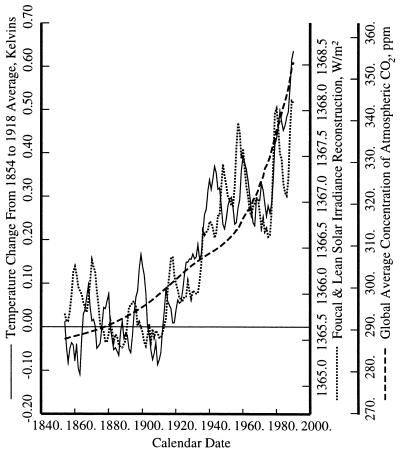
Both CO₂ and changes in solar irradiance have been invoked to explain the observed increase in global temperature. Fig. 1 shows the filtered Jones–Wigley global temperature series, T_g(t) together with a least-squares fit to it using C(t) plus a constant, and a second least-squares fit to T_g(t) using L(t) plus a constant. Each of these fits explains more than 75% of the variance over the full 1854–1990 interval (the residual SDs are 74.2 mK and 83.8 mK, respectively). Including both C(t) and L(t) simultaneously as explanatory variables further reduces the residual SD to 62.5 mK. Nearly 87% of the variance is explained, and both partial F statistics (18) are highly significant, so neither variable can be dropped. Examining these residuals further, one finds that their autocorrelation at a 1-year lag is 0.914 so that the conditions required for the Gauss–Markov theorem (the basis of least-squares) to be valid (19) are not satisfied. This is not simply a technical mathematical quibble, but indicates serious fitting problems whose existence may be verified by repeating the fitting process over different time intervals and observing the change in the estimated coefficients. For example, a least-squares fit to T_g(t) with just the proxy solar irradiance L(t) and a constant the interval 1854–1918 gives a negative temperature response to increasing proxy solar irradiance. Consequently, one must use statistical time-series methods that are reliable when serially correlated residuals are present.

Figure 1.

The Jones–Wigley global temperature series, low-pass filtered to a time resolution of 1 year, with independent least-squares fits to solar irradiance changes and to atmospheric CO₂.

Mathematical Preliminaries

Many of the problems in the analysis of climate data require new methods for time-series analysis. Most of the commonly used time-series methods were derived under the assumption of stationarity, that is, their derivations assume that the statistics of the observed process are independent of the choice of time origin. The climate seems to be nonstationary; over a few years the annual cycle of the seasons makes cyclo-stationary (or periodically correlated) processes a better model than stationary processes, implying that Fourier transforms of frequencies offset by multiples of one cycle per year will be correlated. On longer time scales, evolution of the Earth’s orbit obviously results in vast shifts in the climate, and I recently have shown (2) that these changes in the orbit must be considered in the analysis of instrumental data series as well. Here these effects are accounted for in the way the data were filtered. Because both solar and CO₂ effects alter the seasonal cycle as well as low frequencies, I have not removed common modulation terms at 0 and 1 cycle/year. Finally, anthropogenic changes are altering the composition of the atmosphere and the climate system. Thus, analysis methods that contain an implicit assumption of stationarity should be used with caution.

Similarly, confidence intervals for parameters derived from time series are often based on an assumed Gaussian distribution. It appears that this assumption is invalid for climate data: there are outliers, predominantly from volcanic effects, and, surprisingly, some quantities appear to be more stable than one would expect from a Gaussian distribution.

Even discounting the intrinsic complications of the climate and solar data, the available data is far from homogeneous. There are, for example, no direct measurements of solar irradiance, and only a few direct CO₂ measurements before 1958. In addition, the spatial coverage of the temperature averages has changed markedly. Fluctuations in the fossil-fuel production series (14) appear to be roughly proportional to the level of production, so the absolute errors in the 19th century were lower than they are at present.

The methods used in this paper are a mixture of time-domain and frequency-domain techniques. The multiple-window (20–22) method of spectrum estimation is used as an indirect basis for most estimates. This basic method is formally extended in several ways: Repeating the analysis with each window omitted in turn, or jackknifing over windows (23), gives estimates of the variances of spectra and coherences that do not depend on a Gaussian assumption. Quadratic-inverse theory (24) tests for correlations between closely spaced frequencies, and a variant (25) allows checking for nonstationary effects. The singular value decomposition of a multiple-window spectrogram (21) provides insight into some of the stationarity issues. In addition, a variety of prewhitening and robust estimation methods typified by those in (26, 27) have been used throughout. The Jones–Wigley data, however, has been so carefully prepared that robust procedures detect little more than volcanic activity and do not significantly change the results. Space limitations preclude including many of these checks and comparisons, and I have omitted those that give expected results.

The stochastic structure of both climate and solar data is amazingly complicated when compared to that commonly encountered in textbook examples or even most engineering problems. Because analysis methods for nonstationary time series do not appear to be well enough developed to cope with these series, nor the stochastic structure of the data well enough understood, I use methods that allow simple models for the trends and forcings while leaving nearly stationary residuals.

Stochastic Properties of the Data Series

Because one cannot reliably estimate the relationships between random series without understanding their internal structure, I began this study with a brief examination of the properties of the individual data series. Power spectra of the various series have the usual “red” characteristics of much geophysical data and are not shown. Most of the high-energy, low-frequency part of the spectrum is a result of the trends under consideration, and the stochastic structure is more obvious if the data are prewhitened by filtering. Because the spectra appear similar, I computed the geometric mean of the spectra of T_g(t), L(t), and C_L(t), Fourier transformed this average spectrum to give an autocorrelation sequence, then computed a fourth-order autoregressive prewhitening filter from the autocorrelations. I then use this AR-4 filter on all the data series and recompute the spectra. The spectra have been computed with a multiple-window (20) estimate typically using a time-bandwidth product of 6.0 and the 10 lowest-order windows so the spectrum estimates have a nominal χ-square distribution with 20 degrees of freedom. Their 5% and 95% confidence intervals have been determined by jackknifing over windows (23). The jackknife method is known analytically to give good performance over a range of distributions, to be reasonably distribution free, and, empirically, to be sensitive both to unresolved structure in the spectrum and to nonstationarity. The jackknife variances of the spectrum of the prewhitened temperature series are, on average, about 87% of that expected under Gaussian theory (28).

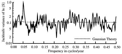
In contrast, the jackknife variance of the spectrum of L(t), Fig. 2, is nearly 10 times that expected near the 22-year Hale cycle and considerably lower than expected around the 11-year sunspot cycle. In a stationary Gaussian series such excursions would be extremely rare.

Figure 2.

The estimated jackknife variance of the natural log of the spectrum of solar irradiance changes. The dashed curve is the expected value and varies slowly as the adaptive weighting process changes the degrees-of-freedom of the spectrum estimate. Note the high peak near the 22-year Hale cycle and the low variance near the 11-year cycle, 0.09 cycle/year.

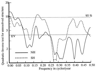
Examining the cause for the low jackknife variance, the quadratic-inverse test for unresolved spectral details (24), Fig. 3, for the Northern Hemisphere is lower than expected except at low frequencies. (The geometric mean, across frequencies, is 3.1, compared to an expected value of 4, and the estimate is below the expected value over much of the frequency range.) This implies that the sampling variations within the analysis bandwidth in the estimated spectrum are smaller than one would expect in a Gaussian random process with a constant spectrum. From this, I infer that much of the apparently random structure in the temperature data is not random but, more probably, a consequence of either deterministic forcing or internal oscillations. Because of the similarity between the statistics of the solar and temperature data, and the stationary temperature residuals (described below), solar forcing is a more likely explanation than internal oscillations. The unresolved structure test in both hemispheres have local maxima near the 22-year Hale cycle and significant maxima at low frequencies.

Figure 3.

Quadratic-inverse tests for unresolved spectral details for the prewhitened Northern and Southern Hemisphere temperature series. The distribution of the test statistics is approximately χ₄² and the dotted lines show the expected value and 95% levels. Note that the Northern Hemisphere estimate is lower than expected over much of the frequency range.

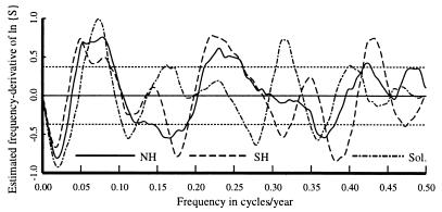
Fig. 4 is a plot of an estimate of the frequency derivative d/df ln{S(f)} [strictly, the relative quadratic-inverse coefficients, b₁(f)/S̄(f) in the notation of ref. 24] for the two hemispheric temperature series and L(t). The higher-order coefficients have similar characteristics, but lower amplitudes. The similarity of the low-frequency features in the temperature and irradiance data lend credence to many of the suggested solar-climate relations and also imply that extracting the statistical details of these relationships will be complicated and difficult.

Figure 4.

Stationary quadratic-inverse coefficients, b₁(f)/S(f), for the Northern and Southern Hemispheres and solar irradiance. The dashed lines near ±0.4 are one SD from the mean for a Gaussian process with a white spectrum. Note the close tracking between all three series at low frequencies and of the temperature series generally.

Turning to the low-frequency maximum in Fig. 3, narrower bandwidth spectrum estimates hint at unusual activity at low frequencies in both T_n and T_s. The harmonic F-test shows moderate evidence for a periodic component with an estimated period of 180 years. The estimated period is longer than the length of the data series, and while the nominal significance level is 99.7%, this is not much higher than 1 − 1/N = 0.993, the level where one expects at least one false detection of a line in noise. However, because the ±1 − σ confidence interval on the period of 153 to 220 years includes the 208-year Suess period, the signal is detected in both hemispheres, and the magnitude-squared coherence between them is about 0.6, the possibility that there is a complicated natural signal in the data near a period of 200 years should not be dismissed. The similarity of the filtered amplitude estimates, 4.4 mK and 4.0 mK, and phases, −135.0° and −138.5° (referenced to 1900.0), in the Northern and Southern Hemispheres, respectively, further support this conclusion. Analysis of long series of ¹⁴C data (21) shows significant components at periods of 230.6, 208.4, and 199.4 years, so because the frequency difference between the latter two periods corresponds to 4,600 years, one cannot expect these components to be resolved in the 137-year series, nor the single line F-test to work reliably.

A possible alternative explanation to deterministic forcing as the cause of the low variances of the temperature spectra is nonstationarity, and this was tested for using the methods in ref. 25. This test shows less variability in time than expected at periods longer than 8 years. Thus, near the 11-year solar cycle, both the tests for unresolved structure and stationarity show more stability than one would expect in a random series. Examination of the nonstationary quadratic-inverse coefficients, a_m(f), shows that the a₂(f)s, approximately, the second time-derivatives of the spectra† are reasonably significant and similar in both hemispheres.

Looking at details of the spectrum of the solar irradiance series, L(t), the predominant feature is the character of the jackknife variance (Fig. 2). There is significant excess variability near 22-year periods and a paucity around 11-year periods. The unresolved structure test is uniformly higher than expected out to a frequency of about 0.13 cycle/year, that is, until the high-frequency edge of the 11-year band, followed by a low region. The nonstationary quadratic-inverse coefficient a₁(f), roughly the time-derivative of the spectrum, or Ṡ(f) in both hemispheres shows decreasing power near 22-year periods and increasing power in the 7- to 11-year period band.

The singular value decomposition of the log-spectrogram described in ref. 21 suggests mild nonstationarity in T_n(t), T_s(t), and L(t) concentrated about the 104-year Suess period, and possibly related frequencies. The phases of the annual cycle of the temperature data shows similar characteristics. Note that this 104-year period is not a simple additive term, but a periodic modulation of the stochastic structure of the process.

I emphasize that the statistical peculiarities just described are those of the individual data series; they contrast markedly with the statistics of the temperature residuals to be described. To the extent that the climate has a linear response to forcing, nonstationarity in the forcing should appear as a similar nonstationarity in the temperature series so, internal oscillations aside, removing the effects of such forcing should leave stationary residuals.

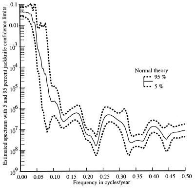
The estimate of the spectrum of the log₂ CO₂(t) data, shown in Fig. 5. shows two important features: first, the range of the spectrum, seven decades, is larger than that of either the temperature or irradiance data, and second, the jackknife variance estimate of ln Ŝ(f) has a maximum of 12.06 at periods near 62 years, compared to an expected value of about 0.13, or 90 times expected. Thus the 5% to 95% confidence region for the CO₂ spectrum estimated by the jackknife method covers a range of about 10⁴, instead of the factor of 2 that would be expected from Gaussian theory. This uncertainty in the spectrum of CO₂ variations carries through to the coherences and transfer function estimates and, consequently, standard frequency-domain estimates of transfer functions are not presented here.

Figure 5.

An estimate of the spectrum of the CO₂ data from 1854–1990 with 5% and 95% confidence intervals determined by jackknifing. The large uncertainty in this estimate precludes making reliable frequency-domain estimates of the transfer functions.

Temperature Response Models and Transfer Function Estimates

I attempted to assess the simultaneous effects of solar variability and greenhouse gases by estimating transfer functions. Because both effects have been advanced as plausible explanations for the increasing temperature, one should expect that changes in solar irradiance and greenhouse gas concentrations should appear coherent as well. It has been shown (29) that, considered as a pair, changes in temperature and CO₂ were coherent, with changes in temperature leading those in CO₂, instead of vice-versa, as popularly supposed. Marland’s fossil-fuel production series, in contrast, leads both the temperature and CO₂ data. Changes in solar irradiance also lead those in both CO₂ and temperature.

In addition to these complicated relationships, there are other difficulties to consider; the physically distributed and multicomponent nature of the problem, combined with spatially and temporally discrete data, makes the appropriate form of the transfer functions obscure. The roughly periodic character of the solar cycle makes lead-lag relations ambiguous. In an attempt to untangle these relationships, I tried several different forms of estimates; the most successful of these is described below. Here I define “successful” as low prediction error, few free parameters, and physically realistic implications. For example, I consider a negative low-frequency response to either increases in solar irradiance or CO₂ unacceptable. Transfer functions implying noncausal response to changes in solar irradiance imply either that the transfer function is unacceptable, or that there is a problem with the assumed irradiance. I also require that the estimates be reasonably insensitive to linear filtering operations applied to the raw data, which eliminates many of the possible models. The rationale for this requirement is two-fold: first, if there is a linear relationship between the input and output of a system, estimates of the transfer function should not change significantly when the same linear filter is applied to both input and output, and second, residuals in the series are autocorrelated, so if the filtering reduces the residual autocorrelation, the requirements of the Gauss–Markov theorem are more nearly satisfied. The estimated transfer functions are clearly not unique, but other acceptable estimates with similar prediction errors have similar implications.

A simple model for the atmospheric CO₂ concentration at time t is

1

where the coefficient ζ on the previous concentration allows for exchange and sequestration by the oceans and biosphere, β is the part of the carbon present in fossil fuels that contributes to atmospheric CO₂, and γ allows for the temperature forcing described in ref. 29. Doing a robust fit with the more accurate Keeling data weighted a factor of 6 higher than the pre-1958 data gives ζ̂ = 0.999974, implying that the atmosphere acts, as expected, as an integrator. The estimated coefficients are β̂ = 0.524, somewhat lower than the estimate in ref. 8 or direct estimates between CO₂ and the integrated fossil fuel record. This is offset by the temperature feedback, γ̂ = 1.196 GT/K. Replacing the T_g(t) term with L(t) gives a slightly poorer fit with a coefficient ≈ 0.38 GT/(W/m²).

In the following paragraphs, I describe some simple time-domain estimates of the transfer functions. If one takes the simplest conceptual model

2

and substitutes Eq. 1 for C(t) one obtains, approximately, the equation

3

with suitable definitions of the constants, and F(t) incorporated into C_L(t). This can be generalized to the class of models

with suitable choices of A, P, and Q. When A = 0 the autoregressive feedback terms are absent, and the model that of a direct finite impulse response filter from L(t) and C(t) to temperature. In particular the models A, P, Q = 0, 1, 0 are the direct least-squares fits, mentioned earlier, to L(t) only; 0, 0, 1 to C(t) only; and 0, 1, 1 to both simultaneously.

I choose the interval 1854–1965 to estimate the coefficients for the particular model and use the 25-year interval, 1966–1990, for validation. Reconsider the direct least-squares estimate model 0, 1, 1. The coefficients obtained by fitting from 1854–1965 are ŝ₀ = 0.1115, ĉ₀ = 1.984. The mean-square error in the fitting period is 6,695 (mK)², or an rms error of 81.8 mK. This fit is not particularly impressive but, nonetheless, it suggests that changes in solar irradiance lead those in temperature by a few years. Using the data for the 25 years 1966–1990, with the coefficients found for the earlier period gives a prediction error of 39,820 (mK)², for an rms error of 199.5 mK. Because the autocorrelations of the residuals in all these cases are large, the assumptions of the Gauss–Markov theorem are violated, and ordinary least-squares does not give reliable results. To see how badly, replace Eq. 2 with

4

where Δ_rT(t) = T(t) − rT(t − 1) and similarly with L and C. Using the 1-year autocorrelation of the temperature data, r = 0.881 for all three series gives s̃₀ = −0.0018, c̃ = 3.121 with corresponding fitting and prediction errors of 1,369 (mK)² and 2,436 (mK)² respectively. Because the innovations variance of the temperature data

where B(v) ≈ 1.07 is a bias correction depending on the degrees-of-freedom (30) of the estimate and Ŝ(f) the estimated spectrum at frequency f, is about 1,303 (mK)² and the variance of Δ_rT is 1,835 (mK)² the errors in Eq. 4 are far less correlated than are those of Eq. 2, so the conditions of the Gauss–Markov theorem are closer to being satisfied. Note that using this simplest of filters on the data increases the estimated sensitivity to C_L by 57% and changes the sign of ŝ₀. Because a decrease in average temperature as a response to an increase in solar irradiance is implausible, I reject such simple models.

Direct frequency-domain estimates of the transfer functions appear to vary too rapidly to be reliably estimated from the available data as their Fourier transforms are significantly noncausal. For example, the impulse response estimated between T_n(t) and L(t) is noncausal with a width about the length of a solar cycle. This is an artifact of the near periodicity of the solar cycle as, without other knowledge or assumptions, one cannot assign the response to a periodic process to a given time without ambiguities of N periods. Similar problems are common in transfer function estimation problems ranging from magnetotellurics (31) to the design of telephone equalizers.

The estimated impulse response between C_L(t) and T(t) is causal and oscillatory with about a 20-year duration. If this characteristic persists with improved early CO₂ data, it implies that large transient responses may be possible.

In addition to thermal inertia, the observed feedback from temperature to CO₂ also generates persistence. To model this together with the effects of CO₂ and solar irradiance changes on the temperature record, I fit the filtered Jones–Wigley series as a 1, 1, 1 model, explicitly Eq. 3. Here the feedback term αT(t − 1) results in a rational (as opposed to polynomial) approximation of the transfer functions allowing more rapid low-frequency changes in them than possible with simple models, it includes some persistence, and generally permits simple feedback effects. Direct least-squares estimates of the coefficients and some performance measures are given in Table 1.

Table 1.

The estimated parameters for Eq. 3 for the three temperature series considered

Temperature series	α	s	c	–1965, mK	1966–, mK
Northern Hemisphere	0.8965	0.0106	0.200	37.1	34.7
Southern Hemisphere	0.8122	0.0033	0.426	32.4	25.1
Global	0.8817	0.0069	0.255	30.4	26.9

The column headed –1965 gives the rms error in the modeling period, 1854–1965. The column headed 1966– gives the rms errors for a 1-year prediction using the parameters estimated from the 1854–1965 and averaged over the 25-year validation interval, 1966–1990. 

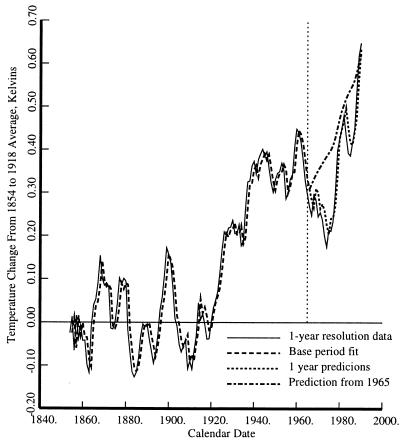
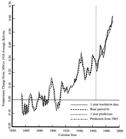
To assess the model’s predictive power I start at 1966 and iterate forward to t = 1990 using the observed solar irradiance and CO₂ data. The predictions were run in two ways: in the first, the temperature data from the previous year was used; in the second, the model was started with the 1965 temperatures and the prediction of the previous year’s temperature used from there on. The 1966– errors in Table 1 refer to the first case. The second is not as accurate, but is not ridiculously inaccurate either; for example, the 25-year prediction of the 1990 Northern Hemisphere temperature is 622 mK, not too dissimilar to the 648 mK observed.

The data, fit, and extrapolations obtained with these models are shown in Fig. 6 (Northern Hemisphere), and Fig. 7 (Southern Hemisphere). The general 25-year prediction agrees reasonably well with the observed temperature in level, if not in exact details. It might be noted that the autoregressive nature of the feedback term in these models causes them to be biased slightly toward zero.

Figure 6.

The Northern Hemisphere temperature data, solid line, and fits. The model coefficients were determined using data before 1965 with the fit shown by the dashed line. After 1965 the fit includes C_L(t), L(t) and the previous year’s temperature. The smoother line, short dashes, shows the prediction starting with the 1965 temperature using only C_L(t) and L(t).

Figure 7.

The Southern Hemisphere temperature and fits. The curves are as in Fig. 6.

Examination of the residuals from this model shows them to be mundane and the exotic characteristics of the individual series missing.

First, the residuals show no significant departures from normality; their range is ±2.35 σ for the global series, there is no detectable skewness, and the standardized fourth moment is 2.65 for the 1854–1965 data, and similar in the validation interval. The Southern Hemisphere residuals are slightly long-tailed. The extreme residual, −107 mK, is a result of the Krakatau eruption in 1883. Thus the errors of 30.4 mK and 26.9 mK obtained for the global temperature with a model having only four parameters imply that the 1990 temperature of 636 mK is about 21 SD above the 1854–1918 base level measured on the scale of the residual SD. The feedback term, αT(t − 1) in Eq. 3, reduces this to about a 9.3σ increase above what persistence would normally generate. The probability of a Gaussian random variable being 9σ from the mean is about 10⁻¹⁹.

Second, the range of the spectrum of the residuals from this model is only 18, just slightly larger than expected for a white-noise process. This spectrum hints at a weak 4.6-year echo-like term.

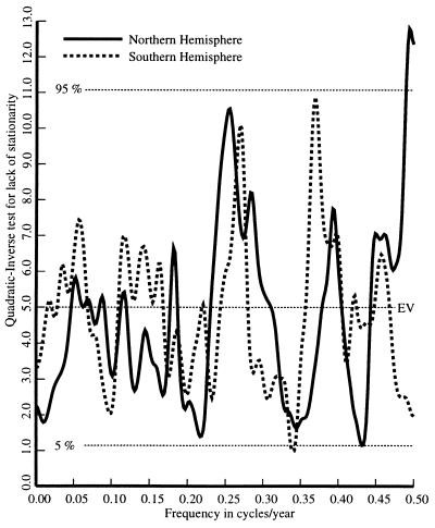
Third, the residuals were tested for stationarity using the quadratic-inverse methods of ref. 25 and, generally, see Fig. 8, the test statistics are slightly less than their expected value, suggesting that the residuals due not contain any serious nonstationary terms. There are, nonetheless, some features of interest. The “time derivative” of the spectrum a₁(f)/a₀(f) is mostly negative, implying that the residual spectrum is decreasing as a function of time. This probably reflects nothing more than the improvements in spatial coverage and data quality that have occurred over the course of the record. The tests for both hemispheres show significant nonstationarity at periods of 4 years, perhaps an artifact of leap years in the original monthly averaging process. In addition, the Southern Hemisphere test has a significant peak in the El-Nino band, and the Northern Hemisphere data are quite nonstationary at the quasibiennial oscillation frequency. At low frequencies, the test statistics from both hemispheres are well below their expected value. Thus the tests for stationarity reveal no evidence for long-term unexplained variability.

Figure 8.

Quadratic-inverse tests for stationarity of the Northern Hemisphere (solid) and Southern Hemisphere (dashed) temperature residuals from model Eq. 3. The test statistics have an approximate χ₅² distribution and have been slightly smoothed for plotting. In both hemispheres the test statistic at a 4-year period exceeds the 98% level.

The transfer functions for this model are

for solar irradiance, and similarly for C_L. The long-term response is given by the low-frequency response; evaluated at f = 0 with the coefficients estimated above one obtains 0.109K/(W/m²) for solar irradiance changes and 2.075 K/(2 × CO₂). To simplify the comparison of the different units one may examine the low-frequency variance explained for the two components and |H_C(0)|²σ_c² = 22,536 (mK)² and |H_S(0)|²σ_I² = 6,067 (mK)² in the Northern Hemisphere, with corresponding figures of 28,320 (mK)² and 317 (mK)² in the Southern Hemisphere. Thus CO₂ explains over 3 times as much variance in changes in solar irradiance in the Northern Hemisphere, over 100 times as much in the Southern. Using simply the change in CO₂ concentration from 287.7 in 1854 to 352.7 parts per million in 1990 the low-frequency transfer function predicts an increase of 0.61 K for CO₂ while an irradiance change of 2.4 W/m² (from 1365.7 to 1368.1 W/m² results in an estimated temperature change of 0.26 K.

Given the great improvement that the addition of the feedback term makes on the direct least-squares estimates, it seems reasonable to investigate related models. A suite of such models, incorporating a range of time delays and prewhitening filters was tested. None of these simple models significantly improve on Eq. 3.

Changes in the Timing of the Annual Cycle

I presented evidence (2) that the frequency of the annual temperature cycle at many locations is closer to the anomalistic year than it is to the tropical year, and, in addition, the character of the phase of the annual cycle began to change rapidly near the middle of this century with the average change in phase coherent with the changes in atmospheric concentration of CO₂. I also suggested that the cause of the rapid phase shift was the changing balance between direct insolation at a given latitude and transported energy. Recall that, at temperate latitudes, the periodicity of insolation is the tropical year and peaks at the summer solstice. The total radiation received by the earth, on the other hand, has the periodicity of the anomalistic year and is maximum at perihelion, currently in early January. In the Northern Hemisphere the phases of the two components are thus nearly opposed and, consequently, the phase of the resultant is easily perturbed. The Sable Island example shown in ref. 6 demonstrates that the proposed mechanism can explain the rapidly changing phase seen at individual stations. The geographic distribution of these phase changes is available in (32, 33), and confirmatory changes are directly observable in the CO₂ record (34).

The observed phase changes must be taken seriously as an indicator of climate change caused by increasing concentrations of atmospheric CO₂. First, the increasing variability of the phases and the change in distribution (Fig. 4 of ref. 2) is so large that the probability of such an occurrence in a stationary process is nearly zero. Second, because the effects of observational errors and similar noise-like effects on the data will be uncorrelated between the low frequencies where the increase in temperature is observed and the annual cycle, one must consider them as independent evidence for a changing climate.

Discussion and Conclusions

More effort must be made to obtain improved CO₂ data for the 19th and early 20th centuries if possible. Similarly, extensive effort to develop better, or independent, solar irradiance proxies is desirable.

Analysis of the low-frequency and annual parts of the temperature records yield at least three largely independent indicators of climate change; the change in distribution of individual station phase trends about the mean, the change in average phase, and the increase in average temperature. All are unprecedented in the instrumental record.

The probability of the observed changes occurring through natural, as opposed to anthropogenic, causes appears to be exceedingly small. First, although a major ice age causes a larger temperature change than has happened so far in response to CO₂, the temperature increase that occurred between 1920 and 1990 would have taken more than 2,000 years even at the historically rapid rate of the last deglaciation. During deglaciation, transient warming in the North Atlantic after a Heinrich event was faster (35), but there is no evidence for a Heinrich event during the last few centuries. Second, internal climate oscillations, shifts in storm tracks, and the like obviously can change local and regional climate by much larger amounts than observed in the hemispheric averages. These regional fluctuations appear to be superimposed on the general global trend. Additionally, such internal oscillations produce warm and cool regions that interchange over decade to century time scales (32, 36), but whose effects largely cancel in hemispheric averages. Third, while there is reasonable evidence for greater climate variability during the Holocene than has been observed during the period where instrumental data are available (37, 38), there is no evidence in the statistics that a major unidentified source of natural variation is present during the instrumental record. Such a source would have to mimic, perversely, either solar irradiance changes or the changes in atmospheric CO₂ to cause the observed temperature changes and to be mistaken for them. Similarly, while mindful of the many caveats on data quality, spatial coverage, etc. given in ref. 1, the appearance of possible leap-year artifacts at a level below 10 mK in the residuals suggests that the data cannot be as untrustworthy as is occasionally implied. The residual temperature variation remaining once the known effects of precession, solar irradiance changes, and atmospheric CO₂ concentration are removed bound unknown effects to about 200 mK peak-to peak in the hemispheric average series during the last century.

Consider the null hypothesis that the observed temperature fluctuations and atmospheric CO₂ levels are independent: The probability that the hemispheric temperatures would fluctuate purely by chance in such a way to produce the observed coherences with CO₂ is exceedingly low. Given that the records encompass more than a century, the probability is so low that one would not expect to see such an event by chance during the age of the earth. The probability of the observed coherence between atmospheric CO₂ and changes in the timing of the seasons shown in figure 13 of ref. 2 without a causal connection is similarly low. Consequently one must strongly reject the hypothesis of independence between atmospheric CO₂ and temperature. The alternative hypothesis, that increasing levels of atmospheric CO₂ plus a slight change in solar irradiance are causally responsible for the observed changes in temperature, in contrast, results in test statistics that are ordinary in every way. Because major changes in climate as a response to human use of fossil fuels have been predicted for more than a century (39, 40), their detection can hardly be considered surprising.

From examining the data records I conclude: Changes in solar irradiance explain perhaps one-quarter of the increase in temperature during the last century. The changes in atmospheric CO₂ concentration resulting from human consumption of fossil fuels cause most of both the temperature increase and the changes in the seasonal cycle.

References

- 1.Houghton J T, Meira Fihlo L G, Callender B A, Harris N, Kattenberg A, Maskell K. Climate Change 1995. Cambridge, U.K.: Cambridge Univ. Press; 1996. [Google Scholar]
- 2.Thomson D J. Science. 1995;268:59–68. doi: 10.1126/science.268.5207.59. [DOI] [PubMed] [Google Scholar]
- 3.Santer B D, Taylor K E, Wigley T M L, Penner J E, Jones P D, Cubasch U. PCMDI Rep. 21. Livermore, CA: Lawrence Livermore Nat. Lab.; 1995. [Google Scholar]
- 4.Schwartz S E, Andrae M O. Science. 1996;272:1121–1122. [Google Scholar]
- 5.Jones P D. J Climate. 1994;7:1794–1802. [Google Scholar]
- 6.Karl T R, Jones P D, Knight R W, White O R, Mende W, Beer J, Thomson D J. Science. 1996;271:1879–1883. [Google Scholar]
- 7.Sonett C P, Giampapa M S, Matthews M S, editors. The Sun in Time. Tucson: Univ. of Arizona Press; 1991. [Google Scholar]
- 8.Keeling C D, Bacastow R B, Carter A F, Piper S C, Whorf T P, Heimann M, Mook W G, Roeloffzen H. In: Aspects of Climate Variability in the Pacific and the Western Americas. Peterson D H, editor. Washington, DC: American Geophysical Union; 1989. pp. 165–363. [Google Scholar]
- 9.Robock A. Science. 1996;272:972–973. [Google Scholar]
- 10.Haigh J D. Science. 1996;272:981–986. doi: 10.1126/science.272.5264.981. [DOI] [PubMed] [Google Scholar]
- 11.Bradley R S, Jones P D. Climate Since AD 1500. London: Routledge; 1992. [Google Scholar]
- 12.Boden, T. A., Kaiser, D. P., Sepanski, R. J. & Stoss, F. W. (1994) Trends ’93: A Compendium of Data on Global Change Pub. ORNL/CDIAC-65, (Oak Ridge National Laboratory, Oak Ridge, TN).
- 13.Manabe S, Wetherald R T. J Atmos Sci. 1967;24:241–259. [Google Scholar]
- 14.Marland, G., Anders, R. J. & Boden, T. A. (1994) Trends ’93: A Compendium of Data on Global Change Pub. ORNL/CDIAC-65, (Oak Ridge National Laboratory, Oak Ridge, TN), pp. 505–584.
- 15.Foukal P, Lean J. Science. 1990;247:347–357. doi: 10.1126/science.247.4942.556. [DOI] [PubMed] [Google Scholar]
- 16.Friis-Christensen E, Lassen K. Science. 1991;254:698–700. doi: 10.1126/science.254.5032.698. [DOI] [PubMed] [Google Scholar]
- 17.Hansen J, Lebedeff S. J Geophys Res. 1987;92:13345–13372. [Google Scholar]
- 18.Draper N R, Smith H. Applied Regression Analysis. New York: Wiley; 1981. [Google Scholar]
- 19.Seber G A F. Linear Regression Analysis. New York: Wiley; 1977. [Google Scholar]
- 20.Thomson D J. Proc IEEE. 1982;70:1055–1096. [Google Scholar]
- 21.Thomson D J. Philos Trans R Soc London A. 1990;330:601–616. [Google Scholar]
- 22.Percival D B, Walden A T. Spectral Analysis for Physical Applications: Multitaper and Conventional Univariate Techniques. Cambridge, U.K.: Cambridge Univ. Press; 1993. [Google Scholar]
- 23.Thomson D J, Chave A D. In: Advances in Spectrum Analysis. Haykin S, editor. Englewood Cliffs, NJ: Prentice–Hall; 1991. , Chapter 2. [Google Scholar]
- 24.Thomson D J. Philos Trans R Soc London A. 1990;332:539–597. [Google Scholar]
- 25.Thomson D J. Proc SPIE. 1993;2027:236–244. [Google Scholar]
- 26.Thomson D J. Bell System Tech J. 1977;56:1769–1815. and 1983–2005. [Google Scholar]
- 27.Kleiner B, Martin R D, Thomson D J. J R Stat Soc. 1979;B-41:313–351. [Google Scholar]
- 28.Thomson, D. J. (1994) in Proc. IEEE Int. Conf. on Acoustics, Speech and Signal Processing, Adelaide, Australia 6, 73–76.
- 29.Kuo C, Lindberg C R, Thomson D J. Nature (London) 1990;343:709–714. [Google Scholar]
- 30.Jones R H. J Am Stat Assoc. 1976;71:386–388. [Google Scholar]
- 31.Larsen J C. Philos Trans R Soc London A. 1992;338:169–236. [Google Scholar]
- 32.Mann M E, Park J. J Geophys Res. 1994;99:25819–25833. [Google Scholar]
- 33.Mann M E, Park J, Bradley R S. Geophys Res Let. 1996;23:1111–1114. [Google Scholar]
- 34.Keeling C D, Chin J F S, Whorf T P. Nature (London) 1996;382:146–149. [Google Scholar]
- 35.Bond G, Broecker W, Johnsen S, McManus J, Labeyrie L, Jouzel J, Bonani G. Nature (London) 1993;365:143–147. [Google Scholar]
- 36.Mann M E, Park J. Nature (London) 1995;378:266–270. [Google Scholar]
- 37.Overpeck J T. Science. 1996;271:1820–1821. [Google Scholar]
- 38.O’Brien S R, Mayewski P A, Meeker L D, Meese D A, Twickler M S, Whillow S I. Science. 1995;270:1962–1964. doi: 10.1126/science.267.5195.257. [DOI] [PubMed] [Google Scholar]
- 39.Arrhenius S. Philos Mag. 1996;41:237–276. [Google Scholar]
- 40.Uppenbrink J. Science. 1996;272:1122. [Google Scholar]