HapCompass: A Fast Cycle Basis Algorithm for Accurate Haplotype Assembly of Sequence Data

Abstract

Genome assembly methods produce haplotype phase ambiguous assemblies due to limitations in current sequencing technologies. Determining the haplotype phase of an individual is computationally challenging and experimentally expensive. However, haplotype phase information is crucial in many bioinformatics workflows such as genetic association studies and genomic imputation. Current computational methods of determining haplotype phase from sequence data—known as haplotype assembly—have difficulties producing accurate results for large (1000 genomes-type) data or operate on restricted optimizations that are unrealistic considering modern high-throughput sequencing technologies. We present a novel algorithm, HapCompass, for haplotype assembly of densely sequenced human genome data. The HapCompass algorithm operates on a graph where single nucleotide polymorphisms (SNPs) are nodes and edges are defined by sequence reads and viewed as supporting evidence of co-occurring SNP alleles in a haplotype. In our graph model, haplotype phasings correspond to spanning trees. We define the minimum weighted edge removal optimization on this graph and develop an algorithm based on cycle basis local optimizations for resolving conflicting evidence. We then estimate the amount of sequencing required to produce a complete haplotype assembly of a chromosome. Using these estimates together with metrics borrowed from genome assembly and haplotype phasing, we compare the accuracy of HapCompass, the Genome Analysis ToolKit, and HapCut for 1000 Genomes Project and simulated data. We show that HapCompass performs significantly better for a variety of data and metrics. HapCompass is freely available for download (www.brown.edu/Research/Istrail_Lab/).

1. Introduction

High-throughput DNA sequencing technologies are producing increasingly abundant and long sequence reads. Third generation technologies promise to output even longer reads (up to a few kb) with increasingly long insert sizes. While the latter promises to alleviate many of the difficulties associated with high-throughput sequencing pipelines, both technologies suffer from producing haplotype phase ambiguous sequence reads. Determining the haplotype phase of an individual is computationally challenging and experimentally expensive; but haplotype phase information is crucial in bioinformatics workflows (Tewhey et al., 2011; Browning and Browning, 2011), including genetic association studies and identifying components of the missing heritability problem (e.g., phase-dependent interactions like compound heterozygosity [Krawitz et al., 2010; Pierson et al., 2012]), the reconstruction of phylogenies and pedigrees, genomic imputation (Marchini and Howie, 2010), linkage disequilibrium, and SNP tagging (Tarpine et al., 2011).

Two categories of computational methods exist for determining haplotypes: haplotype phasing and haplotype assembly. Given the genotypes of a sample of individuals from a population, haplotype phasing attempts to infer the haplotypes of the sample using haplotype sharing information within the sample. In the related problem of genotype imputation, a phased reference panel is used to infer missing markers and haplotype phase of the sample (Marchini and Howie, 2010). Methods for haplotype phasing and imputation are based on computational (Halldórsson et al., 2004) and statistical inference (Browning and Browning, 2011) techniques, but both use the fact that closely spaced markers tend to be in linkage disequilibrium and smaller haplotypes blocks are often shared in a population of seemingly unrelated individuals.

In contrast, haplotype assembly builds haplotypes for a single individual from a set of sequence reads (Schwartz, 2010). After mapping the reads on a reference genome, reads are translated into haplotype fragments containing only the polymorphic single nucleotide polymorphism (SNP) sites. A fragment covers a SNP if the corresponding sequence read contains an allele for that SNP. Because DNA sequence reads originate from a haploid chromosome, the alleles spanned by a read are assumed to exist on the same haplotype. Haplotype assembly algorithms operate on either a SNP-fragment matrix containing a row for each fragment and columns for SNPs or an associated graph that models the relationship between fragments or their SNP alleles.

A considerable amount of theory and algorithms have been developed for the haplotype assembly problem (Halldórsson et al., 2004; Schwartz, 2010; Lippert et al., 2002). The basic combinatorial optimization approach for solving haplotype assembly problems was defined in Lancia et al., 2001. The paper proposed three models of error correction and established NP-completeness of these optimizations; the literature since have designed algorithms employing these error model optimization formulations. For example, some authors have considered restricting the input to sequences of small read length or without mate pairs (termed gapless fragments) (Lancia et al., 2001; Rizzi et al., 2002; Bafna et al., 2005; Li et al., 2006; He et al., 2010). These models, however, are often unrealistic for current high-throughput and future third generation sequence data. Moreover, gapless fragment models are particularly problematic as paired-end sequencing is required to cover SNP alleles that are spaced at distances longer than the sequencing technology's read length. Other combinatorial and statistical algorithms have been developed for general data that relax the optimality constraint (Panconesi and Sozio, 2004; Bansal et al., 2008; He et al., 2010; DePristo et al., 2011). For example, HapCut, computes maximum cuts on a graph modeled from the fragment matrix to iteratively improve their phasing solution (Bansal and Bafna, 2008). Several of these methods were developed when Sanger was the abundant form of sequencing and thus it is unclear whether they can handle massive data on the scale of the 1000 Genomes Project data and beyond. In this paper we test this hypothesis for two leading haplotype assembly algorithms: the Genome Analysis ToolKit's read-backed phasing algorithm (DePristo et al., 2011) and HapCut (Bansal and Bafna, 2008). For a survey of these approaches, see Schwartz (2010).

In this article, we (1) present novel algorithms for haplotype assembly from genome sequencing data. Our algorithms, collectively termed HapCompass, impose no prior assumptions on the input structure of the data and are generally applicable to next-generation sequencing technologies. (2) We compare HapCompass on benchmark sequence data with the two leading software packages capable of producing haplotype assemblies on large data: HapCut and the Genome Analysis ToolKit's (GATK) read-backed haplotype phasing algorithm. We show that HapCompass is faster and significantly more accurate than HapCut and GATK using a variety of metrics on real and simulated data. (3) We present simulations to highlight the type of data needed to supplement existing 1000 Genomes Project data to completely phase a chromosome.

2. Methods

2.1. Graph theory models for haplotype assembly

The input to the haplotype assembly problem is a set of DNA sequence reads for a single individual. Sequence reads are mapped to the reference genome to identify the SNP content of the reads. A fragment is a mapped sequence read that has the non-polymorphic bases removed. SNPs for which the individual is homozygous are not useful for assembly because a fragment containing either allele cannot uniquely identify which haplotype the allele was sampled from. Furthermore, fragments containing zero or one heterozygous SNPs—while potentially useful for SNP calling—are not useful for the assembly of haplotypes and are discarded as well. Fragments containing two or more heterozygous SNPs contain valuable haplotype phase information as they link together each allele to the same haplotype and define a potential phasing.

Formally, we define the i^th fragment f_i as a vector of {0, 1, − } where 0 and 1 represent the major and minor alleles at some SNP site and “-” represents a lack of information either because the read does not cover the SNP site or there was a technical failure (e.g., in mapping or sequencing). We define an m × n SNP-fragment matrix M whose m rows correspond to fragments and n columns correspond to heterozygous SNPs . Each fragment f_i covers at least two of the n SNP sites; SNPs covered may not be consecutive on the genome (e.g., when the fragments originate from paired reads). We refer to the SNP allele k of f_i as f_i,k. We say that two fragments f_i and f_j are in fragment conflict if

That is, two fragments conflict if they cover a common SNP and have different alleles at that site.

Two fundamental graph models associated to the SNP-fragment matrix M were introduced by Lancia et al. (2001) called the fragment conflict graph and the SNP conflict graph. The fragment conflict graph, G_F(M) = (V_F, E_F), is defined as follows: the vertices are fragments, and the edges are 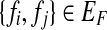if f_i and f_j conflict . For an error-free M, each connected component in G_F(M) has a bipartition and thus the vertices can be divided into two conflict-free disjoint subsets; the subsets define a haplotype phasing for the SNPs associated with the connected component.

The SNP conflict graph, G_S(M) = (V_S, E_S), is defined as follows: the vertices are SNPs, and the edges 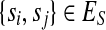if s_i and s_j exhibit more than two haplotypes . If s_i and s_j exhibit three or four haplotypes, then some read covering s_i and s_j contains at least one error because only two haplotypes are possible for a diploid organism. Methods like HASH and HapCut employ different graph models where SNPs correspond to vertices and fragment information is encoded in the edges (Bansal et al., 2008; Bansal and Bafna, 2008). HapCut keeps a reference to the current phasing of the data and each edge is weighted proportional to the number of fragments that cover the adjacent SNPs and agree with the reference phasing.

2.2. A new model: compass graphs

Our algorithms operate on a new undirected weighted graph associated to the SNP-fragment matrix M (similar to the SNP conflict graph and HapCut graph), called the compass graph, G_C(M) = (V_C, E_C, w), defined as follows: (1) the vertices are SNPs, ; (2) the edges are 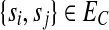if at least one fragment covers both s_i and s_j; and (3) each edge {s_i, s_j} has an associated integer weight w(s_i, s_j). The weight function w is defined by the fragments. Because there exists exactly two phasings between any two heterozygous SNPs for a diploid genome, let us denote the two possible phasings as when the haplotype 00 is paired with the haplotype 11 and similarly denote the other phasing. Our weight function w for a pair of SNPs simply counts the difference between the number of phasings and the number of phasings as defined by the fragments. Formally, let F be the set of all fragments covering two SNPs s_i and s_j. The weight w(s_i, s_j) is defined as follows:

where 1(b) = 1 for b true and 1(b) = 0 for b false. We note that a subgraph of a compass graph is also a compass graph. Figure 1 illustrates the relationship between M and its compass graph G_C(M).

FIG 1.

The SNP-fragment matrix M is shown on the left containing four fragments and four SNPs. Each pairwise phasing relationship defined by the fragments is represented on the edges of the compass graph on the right. A positive edge indicates there is more evidence in the fragments for the phasing while a negative edge indicates evidence for the opposite phasing.

The compass graph G_C encodes information derived from the fragment set regarding the phasings of SNPs in its edge weights. For example, fragments covering three SNPs would provide phasing information for all the edges defined by the fragment in G_C. The collected evidence for an edge may have conflicting information, that is, some fragments may provide evidence for a phasing while other fragments suggest a phasing. An edge with weight of zero occurs when evidence for both phasings between the pair of SNPs is equal and thus both phasings are considered. An edge with a non-zero weight is called decisive. A decisive edge in E_C defines the phasing between its two SNPs which is given by the sign of its weight (i.e., majority rule phasing).

2.2.1 Properties of the compass graph

We can extend unique pairwise phasings of decisive edges of G_C to unique phasings of paths. In other words, the phasing is transitive among the SNPs along a path. An edge of G_C is said to be positive (negative) if its weight is positive (negative).

Lemma 1

There is a unique phasing between two SNPs s_i and s_j if and only if for any two simple edge-disjoint paths p and q in G_C between s_i and s_j, the number of negative edges of p plus the number of negative edges of q is even, and p and q include no 0-weight edges.

Proof 1

If there is a unique phasing between two SNPs s_i and s_j then they must be connected in G_C. If there is only one path between s_i and s_j then the phasing is unique because this one path induces the only phasing between the two SNPs. If there is t >  1 paths between s_i and s_j then there exists a total of pairs of paths. Let p and q be any two paths in the traversal from s_i to s_j. Let p and q have k and l edges with negative weight respectively. If k and l are both odd, the phasing induced between s_i and s_j by both paths is Likewise, if k and l are both even, the phasing induced between s_i and s_j by both paths is If k is odd and l is even, p defines the phasing as and q defines the phasing as (and vice versa in the case of l odd and k even). So if all paths between s_i and s_j produce a total negative edge traversal count that is even, the induced phasings cannot conflict. Likewise, if at least one pair of paths produce a total negative edge traversal count that is odd then at least one pair of paths disagree on the phasings of s_i and s_j. Also, if there is a unique phasing between two SNPs, no paths include a 0-weight edge by definition. The other direction follows similarly.   ■

Definition 1

A conflicting cycle in G_C is a simple cycle that contains either an odd number of negative edges or at least one 0-weight edge or both. A non-conflicting cycle, is called a concordant cycle and contains an even number of negative edges and no 0-weight edges.

Definition 2

A compass graph has a unique phasing if it has no conflicting cycles. We call such a compass graph happy.

The following fundamental relationship between spanning trees and happy compass graphs is encapsulated in the following theorem.

Theorem 1

Every spanning tree of a compass graph is a happy graph. Every spanning tree of a happy compass graph has the same unique phasing as the compass graph.

Figure 2 gives an example of computing a happy compass graph from G_C in one edge removal step. Two spanning trees are shown in the happy G_C which correspond to the same phasing.

FIG 2.

A compass graph G_C is shown on the left with two conflicting cycles. One edge removal (s₂, s₃) makes G_C happy by removing two conflicting cycles in one step. All spanning trees (ST) of the happy G_C correspond to the same phasing, but only two are shown in the lower right corner.

2.3. Problem formulations

Computing the two phased haplotypes consistent with a matrix M is trivial for error free data. When errors are present, error correction may be modeled by: removing a fragment (row), removing a SNP (column), or flipping the matrix entry defined by a particular fragment and SNP (from 0 to 1 or vice versa) (Lancia et al., 2001). Every M induces a particular graph G_F, G_S, and G_C, and error correction models on these graphs yield different formulations of the haplotype assembly problem. There are four problem formulations that have received the most attention in the literature:

• (1/2) Minimum edge/fragment removal (MER/MFR): Remove the minimum number of edges/vertices from the fragment conflict graph G_F(M) such that the resulting graph is bipartite.

• (3) Minimum SNP removal (MSR): Remove the minimum number of vertices from the SNP conflict graph G_S(M) such that no two vertices are adjacent (a graph with no edges).

• (4) Minimum error correction (MEC): Correct the minimum number of errors in fragments of M (by switching the allele from 0 to 1 or vice versa) such that the rows (fragments) of the induced matris M′ can be partitioned into two subsets such that no fragment conflicts exist within each set.

When the input is restricted to gapless fragments (i.e., each fragment covers a contiguous set of SNPs), MFR and MSR can be solved efficiently (Lancia et al., 2001). However, when considering sequence reads with an arbitrary length between an arbitrary number of contiguous blocks of SNPs, MFR and MSR are NP-hard (Lancia et al., 2001). MER is NP-hard for general input (Lippert et al., 2002) and MEC is NP-hard even for gapless instances (Zhao et al., 2005; Lippert et al., 2002).

2.3.1. Minimum weighted edge removal

The minimum weighted edge removal (MWER) optimization problem is defined for a compass graph G_C. Let L ⊂ E_C be a subset of edges in G_C and let be the resulting graph created from removing L from E_C. MWER aims to compute an L such that the following conditions are satisfied: (1) 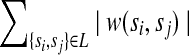is minimal (cost of removed edges is minimal); (2) all edges in are decisive; and (3) choosing a phasing for each edge in by majority rule gives a unique phasing for . Observe that a compass graph that meets conditions (1–3) is a happy graph.

The MWER problem for G_C aims at constructing the phased haplotypes that are most witnessed by the pairwise phasing information contained in the fragments. Removed edges model the tolerance of some conflicting evidence. The final phasing for the retained edges is obtained as a consequence of the global unique phasing of the resulting happy graph.

2.4. Cycle basis algorithms

We present two algorithms for the minimum weighted edge removal problem on compass graphs. Our local improvement algorithms are based on the following data structure. We compute a spanning tree of the compass graph G. The spanning tree cycle basis of G with respect to T is the set of simple cycles obtained by taking each non-tree edge e and constructing the unique cycle in the graph T∪e. This spanning tree cycle basis has cardinality |E_C| − (|V_C| − 1). The HapCompass Algorithm 1 iterates the following steps until the compass graph is happy: (1) select a random conflicting cycle, (2) remove the edge with the least amount of evidence, and (3) rebuild the cycle basis.

Algorithm 1.

1. Remove all 0-weight edges from GC. The removal of edges with 0-weight does not affect the MWER score and can therefore be removed.

2. Construct a maximum spanning tree T.

3. The spanning tree cycle basis is computed in respect to T and cycles are marked as either conflicting or concordant. Iterate (4–6) until GC is happy:

4. Select a conflicting cycle at random and remove the edge e with weight closest to 0; this represents the edge with the least amount of evidence for phasing its SNPs. The removal of e can either remove a tree or non-tree edge of T.

5. If e is a non-tree edge then T is obviously still a valid spanning tree. If e is a tree edge then we add the non-tree edge ent into the spanning tree T. After this step we clearly still have a spanning tree as any path that previously passed through the removed edge e can now pass through the added edge ent.

6. If e was a tree edge, compute a new cycle basis in respect to T ∪ ent. The addition of the non-tree edge into the spanning tree T might introduce conflicts in existing concordant cycles in which case we add these cycles to the set of conflicting cycles. However, the algorithm will continue to remove edges until GC is a tree which is a valid phasing thus the algorithm terminates.

7. Output the phasing corresponding to any spanning tree of GC and the number of weighted edges corrected as the score of this phasing (or output the weight of all remaining edges in GC).

Let m=|E_C| and n = |V_C|, then the number of non-tree edges is |E_C| − |T| = m − n + 1.

Lemma 2

Algorithm 1 runs in O(m(m − n + 1)² + (m − n + 1)(m log n)) time.

Proof 2

The removal of 0-weight edges in step (1) can be done in O(m) time. Step (2) involves computing a maximum spanning tree which can be done in O(m log n) time. For step (3), we keep pointers at each vertex pointing to the “parent” node in respect to an arbitrary root vertex. The algorithm never traverse an edge more than m − n + 1 times. So this step takes no longer than O(m(m − n + 1)). Again, step (4) takes no longer than m(m − n + 1) time for processing all simple cycles in respect to T. Step (5) processes one cycle, so, if the cycle being considered is c, then this operation takes at most |c| time. Step (6) is dominated by O(m log n). For step (7) the algorithm parses through each edge of G_C thus this step takes no more than O(m) time. Because we iterate through steps (4–6) at most (m − n + 1) times the algorithmic complexity is O(m(m − n + 1)² + (m − n + 1)(m log n)).   ■

HapCompass Algorithm 1 presents the basic structure of the cycle basis optimization. In practice we use a more involved algorithm (HapCompass Algorithm 2) that exploits the relationship between MWER and set cover.

Algorithm 2.

• We follow steps (1–3) but replace (4) with a step that removes a set of highly conflicting edges. In the MWER set cover formulation each edge of GC is a set and each conflicting simple cycle is an element. The simple cycle elements belong to an edge set if the edge is part of that cycle. We then formulate the problem of resolving the conflicting cycles as finding the set of edges (sets) of minimum weight such that they cover all of the conflicting simple cycles (elements).

• Each conflicting simple cycle will have at least one edge removed, and, removing one or more edges from a conflicting cycle creates a tree which, due to Lemma 1, is non-conflicting. This, of course, would be too computationally expensive to formulate for the entire graph so we use this step on a subset of cycles. This subset is found by selecting the edge that is a member of the most conflicting cycles (this can easily be logged at the computation of the cycle basis).

• After removing a set of edges, we reconnect T. During the removal of each edge, we find the non-tree edge whose absolute value of the weight is the largest and add it back into T after all edges are removed.

• Steps (6–7) are computed as before.

Lemma 3

At the end of each step, G_S is connected.

Proof 3

If only one cycle was corrected at a time then the non-tree edge selected for inclusion into T provides a new path for vertices previously using the removed edge. If more than one cycle was corrected by the removal of one edge, then paths previously taking the removed edge can now take any non-tree edge associated with the set of cycles.   ■

Lemma 3 is critically important because it ensures we do not needlessly separate components and create haplotype phase uncertainty.

The primary difference between Algorithms 1 and 2 is the local optimization step, where Algorithm 2 removes multiple edges using the set cover formulation; this formulation models a sense of parsimony in that we prefer the removal of edges that resolve multiple conflicting cycles at once.

Lemma 4

If the edge e is shared by k conflicting cycles then the removal of e resolves the k conflicting cycles.

Proof 4

G_C has had all edges with 0-weight removed thus each conflicting cycle has an odd number of negative edges. Let c_i and c_j be any two of the k conflicting cycles with negative edge counts of n_i and n_j. If e is positive then c_i and c_j form a cycle whose negative edge count is n_i + n_j. If e is negative then c_i and c_j form a cycle whose negative edge count is (n_i − 1) + (n_j − 1). In both cases (odd+odd and even+even) a cycle is produced containing an even number of negative weighted edges.   ■

An illustration of Lemma 4 is shown in Figure 2. There are two caveats to Lemma 4 that are due to the complex relationship between sets: (1) the removal of an edge will resolve conflicting cycles but may change concordant cycles into conflicting and (2) the removal of successive edges after the first may revert previously resolved conflicting cycles. These issues arise from the set cover formulation which simply optimizes the sum of the weighted sets and does not consider complex interactions between sets.

There are several ways to address these caveats. We may consider other properties of the edges in our minimum weighted set cover formulation. The weight on an edge e corresponds to the confidence in the pairwise phasing between the two adjacent SNPs of e. Another measure of confidence for e in G_C is the number of conflicting and concordant cycles e is a member of. The weight in the minimum weighted set cover formulation can then be computed as a combination of the edge weight and conflicting/concordant cycle membership. Because the number of conflicting or concordant cycles an edge is a member of may change with the selection of the first covering set, this minimum weighted set cover is solved iteratively. However, in practice, we specifically address (1) by breaking edge-weight ties with the number of conflicting cycles minus the number of concordant cycles and (2) by not considering shared edges from any of the resolved conflicting cycles in future removal steps of the same iteration.

Theorem 2

Algorithm 2 is a polynomial-time algorithm and terminates with G_C a happy graph (i.e., having exactly one phasing).

Proof 5

Algorithm 2 retains Algorithm 1's complexity with additional computation in step (4). The greedy approximation algorithm for set cover, however, can be computed in linear time in the size of the sets so Algorithm 2 is clearly polynomial. Lemma 4 allows the resolution of many conflicting cycles at each local optimization step but may also change existing concordant cycles to conflicting. However, because the graph is connected at the end of each step (Lemma 3) and we correct |E_C| − (|V_C| −1) edges in the worst case, the algorithm clearly terminates. We also have the property that the final happy graph corresponds to a valid phasing because of Lemma 3.   ■

3. Results

Comparison of algorithms that operate under the same error model is straightforward. However, comparing algorithms across different error models is not well defined. Therefore, care must be taken to develop metrics that best capture the more accurate solution independent of the error models employed.

3.1. Evaluation criteria for haplotype assembly

Before we consider new evaluation metrics that capture the quality of the haplotype assembly, we address the haplotype switch error metric that has been used previously when the ground truth is known. The haplotype switch error metric is defined as the number of switches in haplotype orientation required to reproduce the correct phasing (Lin et al., 2002). It was originally developed for the haplotype phasing problem and was among the metrics used in the Marchini et al., 2006 phasing benchmark. Switch error is generally more favorable than pure edit distances for haplotypes because it more accurately models the phase relationship between adjacent SNPs.

This metric was originally developed for haplotype phasing algorithms which operate on the genotype data of many individuals simultaneously. Haplotype sharing and linkage disequilibrium are very important quantities for haplotype phasing algorithms as the relationship among adjacent SNPs allows methods to infer likely haplotypes in the data. In this manner, the switch error metric accurately captures the close range relationship between adjacent SNP phase. However, haplotype assembly algorithms operate on much different data and assumptions. Phase relationships are inferred often from long distance mate pair reads. The switch error metric does not accurately capture these relationships. Furthermore, if two haplotype assemblies do not produce the same amount of blocks of haplotypes or otherwise do not agree on where to commit to a particular phasing, then the switch error becomes biased towards those algorithms that phase less SNPs.

Instead, we suggest using a new metric inspired by genome assembly that captures how well the haplotype assembly represents the input fragments and can be applied regardless of knowing the true haplotypes. One of the most meaningful statistics for genome assembly is how many sequence reads successfully map back to the assembly. We can also slightly modify this metric to ask the question: “How many of the phase relationships represented by the read fragments are represented in the assembly?” This fragment mapping phase relationship (FMPR) metric summarizes how well the haplotype assembly represents the input data.

Let the set of all fragments be F and f_i the i^th fragment of F. We denote the k^th SNP of f_i as f_i,k. The haplotypes produced from an algorithm are denoted h₁ and h₂ and the allele of h₁ at position k is denoted h_1,k (h_2,k is defined similarly). Then the fragment mapping phase relationship metric can be described as

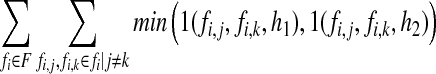where 1() is a function that takes two SNP alleles and a haplotype and determines whether the phase relationship between the two alleles exists in the haplotype; formally, 1( f_i,j, f_i,k, h₁) = 1 if ( f_i,j ≠ “–” ∧ f_i,k ≠ “–”) ∧ ( f_i,j ≠ h_1,j ∨ f_i,k ≠ h_1,k) and 1( f_i,j, f_i,k, h₁) = 0 otherwise. This metric is computed by counting all of the pairwise phase relationships defined by the input set of fragments that do not exist in the solution. One fortunate side effect of this metric is that an algorithm that produces smaller blocks will be penalized. For instance, if an algorithm produces a haplotype assembly for five disjoint blocks when fragments exist in the data that connect every SNP in one large block, the switch error metric will not penalize the unknown phase between blocks. However, the fragment mapping metric will capture the phase ambiguity error that exists between disjoint blocks if the input fragments do indeed suggest they should be connected. We also define the boolean fragment mapping (BFM) metric which counts the percentage of fragments that map to the resolved haplotypes with at least one error (i.e., the number of fragments that do not perfectly map to a phased haplotype). For both FMPR and BFM metrics, smaller numbers are preferred.

3.2. 1000 genomes data

We first evaluate the number of reads that must supplement the current high coverage 1000 genomes data (The 1000 Genomes Project Consortium, 2010) for the NA12878 CEU individual in order to achieve a complete haplotype assembly of chromosome 22. To do this, we supplemented the 454, Illumina, and SOLiD sequence data with simulated Illumina reads. The starting point of each simulated read was generated at random from the set of bases that were sampled by real sequence reads. Illumina-sized reads were simulated using varying distributions for insert size. Figure 3 shows a least squares fitted curve to the largest component (or block) sizes for varying values of coverage for chromosome 22. Disconnected components of G_C must be phased separately and the haplotype phase between them is ambiguous; therefore, the largest component size gives an indication of the connectedness of G_C and the size of the maximum achievable phased haplotype.

FIG 3.

In this simulation study, reads of size 100 bp were simulated on chromosome 22 of the 1000 genomes CEU individual NA12878. Mate pair lengths were sampled at random from one of four normal distribution with means [10 kb, 50 kb, 100 kb, 250 kb] and standard deviations [1 kb, 5 kb, 10 kb, 25 kb]. With these parameters for sequencing, we require about 10 million reads to connect most of the SNPs of G_C.

We then evaluated each algorithm using the aforementioned metrics for the Illumina, SOLiD, and 454 reads generated for the CEU individual NA12878 in the 1000 genomes data (Table 1). Because each sequencing technology produces reads with similar insert sizes, the real data block sizes are small. For these block sizes, HapCompass produces the best results with GATK also producing very accurate haplotype assemblies.

Table 1.

HapCut, GATK, and HapCompass (HC) were Evaluated According to the Fragment Mapping Phase Relationship and Boolean Fragment Mapping Metrics for 1000 Genomes Data Chromosome 22 of Individual NA12878. The Block Size is the Number of SNPs in the Component of G_C and no. Fragments Denotes How many Read Fragments were Used for Assembly. Bold Cells Denote the Algorithm with the Best Score.

block size	no. fragments	HapCut FMPR (BFM %)	GATK FMPR (BFM %)	HC FMPR (BFM %)
51	477	223 (13.8)	60 (8.4)	23 (1.9)
53	581	265 (11)	30 (2.9)	25 (2.4)
53	551	71 (7.1)	23 (2.9)	9 (1.3)
58	626	209 (11)	12 (1.4)	12 (1.4)
60	645	199 (10.1)	54 (3.9)	43 (3.1)
60	467	28 (4.7)	18 (3)	4 (0.86)
62	393	24 (4.5)	14 (3.1)	6 (1.5)
62	528	126 (10.6)	16 (2.5)	8 (1.3)
63	770	45 (3.8)	24 (2.2)	19 (1.7)
66	602	91 (5.6)	31 (3.7)	11 (1.5)
66	718	452 (14.6)	47 (3.3)	28 (2.1)
79	877	245 (10.1)	26 (2.1)	8 (0.8)
102	949	212 (8.7)	48 (2.7)	37 (1.9)
166	1914	207 (5.9)	83 (2.7)	44 (1.5)
Total FMPR	–	2397	486	277

3.3. Simulated data

Limitations in current sequencing technologies restrict the number of SNPs one can hope to phase from the sequence reads. Many factors influence the connectedness of G_C but the most influential factor is the distribution of lengths of the inserts used to generate the paired reads (Halldorsson et al., 2011). This is less of a concern for whole-exome data where haplotype assemblies can be constructed rather easily with high coverage. However, in order to test the algorithms on their capability to provide genome-wide haplotype assemblies in terms of both accuracy and time efficiency, we simulated two datasets of 10 million 100 bp reads and varied the error parameter. The 10 million reads parameter is guided by the data generated for Figure 3 and will vary depending on read length, insert size distributions, coverage, and genome allele structure (e.g., runs of homozygosity that are longer than the insert size will disconnect components of G_C).

Because the NA12878 individual is the child of a CEU trio who were also sequenced, we used the parents to phase most of the SNPs; a random phasing was selected for SNPs that were triply heterozygous. Using this method, we construct a baseline set of haplotypes to simulate reads from that are as close to the ground truth as possible with the available data. Our principle measurements of accuracy are FMPR and BFM. First we tested each algorithm on simulated data with moderately high error rates (0.05).

We can summarize the trends in the results Tables 1 and 2 by fitting a linear least squares regression line to the data (Fig. 4).

Table 2.

HapCut, GATK, and HapCompass (HC) were Evaluated According to the Fragment Mapping Phase Relationship and Boolean Fragment Mapping Metrics for 1000 Genomes Data Chromosome 22 of Individual NA12878 and 10 Million Simulated Reads with Error Rate = 0.05 and Read Length = 100. A Dash (-) Mark Denotes the Algorithm did not Finish Using the Allotted Resources. Bold Cells Denote the Algorithm with the Best Score.

block size	no. fragments	HapCut FMPR (BFM %)	GATK FMPR (BFM %)	HC FMPR (BFM %)
580	2268	355 (13.8)	703 (28.2)	284 (11.4)
1331	4023	647 (14.5)	1236 (28.7)	441 (10.1)
1598	6545	1182 (15.5)	2011 (27.6)	1033 (13.9)
1835	6962	1212 (14.8)	2235 (28.8)	1089 (13.8)
3193	15036	3416 (17.7)	5237 (30)	2746 (15.7)
4153	17862	3642 (16.6)	- (-)	2719 (13.2)

FIG 4.

We fit a linear least squares regression line to the FMPR measurement for algorithms Genome Analysis ToolKit (GATK), HapCut, and HapCompass on chromosome 22 of the 1000 genomes data for the NA12878 individual (top) for the 1000 genomes data only (Table 1) and (bottom) for the 1000 genomes data supplemented with 10 million simulated reads of length 100 and sequence base error rate of 0.05 (Table 2).

It is clear from Figure 4 that HapCompass produces the best results. HapCut seems to produce better results than GATK on larger haplotype blocks (the reverse was true for the small haplotype blocks from real data). When considering serial execution, the processing times for HapCut and HapCompass were similar. For instance, for the simulated component of size 4177, 25 iterations of HapCut took 3.7 hours while 25 iterations of HapCompass took 4.8 hours. However, iterations of the HapCompass algorithm are independent and can be trivially parallelized. When this is the case, the solution with the smallest MWER score is retained as the overall solution. HapCut and HapCompass both used less than 2 gigabytes of memory while GATK required a great deal more memory and processing time for similar sized components. Each algorithm was terminated if it required more than 12 hours of processing time or 8 gigabytes of heap space.

Even though switch error has an unclear interpretation on haplotype assembly data, we show that switch error produces the same algorithmic rankings. Switch error is as defined before but we incur a penalty of 1 for each haplotype block reported beyond the first. Because we compare each algorithm to a connected haplotype block—in the sense that there is a path between every SNP in G_C—reporting more than one phasing represents a switch error between phased components. The switch error metric gives the same relative ranking of algorithm performance (Table 3). We only show these results for completeness and do not recommend using switch error as the sole measurement of haplotype assembly algorithm accuracy.

Table 3.

Switch Error (SE) Measurements for HapCut, GATK, and HapCompass (HC) for the Same Data as Table 2. A Dash (-) Mark Denotes the Algorithm did not Finish Using the Allotted Resources. Bold Cells Denote the Algorithm with the Best Score.

block size	no. fragments	HapCut SE	GATK SE	HC SE
580	2268	197	259	148
1331	4023	544	581	329
1598	6545	604	654	474
1835	6962	694	766	563
3193	15036	1092	1287	859
4153	17862	1630	–	1007

We then reduced the error rate to evaluate the behavior of each algorithm on higher quality data. Table 4 again demonstrates that HapCompass remains significantly better than HapCut and GATK.

Table 4.

HapCut, GATK, and HapCompass (HC) were Evaluated According to the Fragment Mapping Phase Relationship and Boolean Fragment Mapping Metrics for 1000 Genomes Data Chromosome 22 of Individual NA12878 and 10 Million Simulated Reads with Error Rate = 0.01 and Read Length = 100. A Dash (-) Mark Denotes the Algorithm did not Finish Using the Allotted Resources. Bold Cells denote the Algorithm with the Best Score.

block size	no. fragments	HapCut FMPR (BFM %)	GATK FMPR (BFM %)	HC FMPR (BFM %)
578	2326	180 (6.6)	650 (25.5)	46 (1.7)
1852	7234	888 (10.7)	1896 (23.7)	207 (2.5)
4177	17953	2088 (9.3)	- (-)	425 (2)

4. Discussion

The HapCompass algorithmic framework can also be extended to other optimization formulations. For instance, it is possible to extend these algorithms to accommodate the MEC formulation by employing a different local optimization step. However, we do not have the same termination requirements as with MWER. In particular, an edge must have all fragment based evidence suggesting one unique phasing. The MEC optimization also defines a different local optimization sub-problem. Preliminary results are encouraging where we model the local optimization as a haplotype clustering problem; the sub-problem becomes finding the two haplotypes that minimize the MEC on a subgraph of G_C.

As is the case with most haplotype assembly algorithms, our algorithm does not yet consider quality scores of sequence reads or SNP calls. In the previous analyses, we simulated reads with perfect mapping and sequence call quality. This information, however, could be incorporated into the weights on the edges. More precisely, the edges of G_C require a measurement of confidence in the phasing and other sources of information may be encoded on these edges; for instance, a likelihood model may also be formulated accommodating the inclusion of sequence base call scores and the quality of SNP calls.

5. Conclusion

Haplotype assembly is becoming increasingly important as the cost of sequencing plummets and more genome-wide and whole-exome studies are conducted (Levy et al., 2007; Tewhey et al., 2011). We have designed and implemented a haplotype assembly algorithm that is widely applicable to these studies because it does not make any prior assumptions on the input data. Through the use of simulations, we show that supplementing 1000 genomes data with sequencing data of a particular type connects G_C enabling the haplotype assembly of entire chromosomes. We described the fragment mapping phase relationship and boolean fragment mapping metrics that capture the quality of the haplotype assembly through support from mapped fragments. These metrics can be used independent of the algorithm and without knowing the true haplotypes to evaluate the quality of the haplotype assembly.

We compared HapCompass to two leading haplotype assembly software packages that can also process arbitrary input sequence data: HapCut and the Genome Analysis ToolKit's read-backed phasing algorithm. HapCompass is shown to be more accurate on real 1000 genomes data for the BFM and FMPR metrics. We also show that HapCompass is more accurate when we supplement the existing 1000 genomes real data with simulated Illumina reads for BFM, FMPR and haplotype switch metrics on haplotype blocks of unprecedented size. Although only data from chromosome 22 is shown (chr22 with 33144 SNPs), the number of SNPs on the most polymorphic chromosome (chr2 with 218005 SNPs) is only an order of magnitude more according to CEU 1000 genomes data (minor allele frequency ≥ 0.01). Because we have shown the small order polynomial complexity of this algorithm, we do not believe it would be difficult to extend this algorithm to operate on large components of G_C in parallel on a computing cluster for genome-wide data. As high-throughput sequencing becomes more available to a greater number of researchers, we believe HapCompass will provide a valuable tool to quickly and accurately identify the haplotypes of diploid organisms.

Acknowledgments

We thank Bjarni Halldórsson for many helpful early discussions regarding haplotype assembly. This work was supported by the National Science Foundation (grant 1048831 to S.I.; the work of D.A. and S.I. was supported by this grant).

Disclosure Statement

No competing financial interests exist.

References

- Bafna Vi. Istrail S. Lancia G., et al. Polynomial and APX-hard cases of the individual haplotyping problem. Theor. Comput. Sci. 2005;335:109–125. [Google Scholar]
- Bansal V. Bafna V. HAPCUT: an efficient and accurate algorithm for the haplotype assembly problem. Bioinformatics. 2008;24:153–159. doi: 10.1093/bioinformatics/btn298. [DOI] [PubMed] [Google Scholar]
- Bansal V. Halpern A. L. Axelrod N., et al. An MCMC algorithm for haplotype assembly from whole-genome sequence data. Genome Res. 2008;18:1336–1346. doi: 10.1101/gr.077065.108. [DOI] [PMC free article] [PubMed] [Google Scholar]
- Browning S.R. Browning B.L. Haplotype phasing: existing methods and new developments. Nat. Rev. Genet. 2011;12:703–714. doi: 10.1038/nrg3054. [DOI] [PMC free article] [PubMed] [Google Scholar]
- Deo N. Prabhu G. Krishnamoorthy M.S. Algorithms for generating fundamental cycles in a graph. ACM Trans. Math. Softw. 1982;8:26–42. [Google Scholar]
- DePristo M.A. Banks E. Poplin R., et al. A framework for variation discovery and genotyping using next-generation DNA sequencing data. Nat. Genet. 2011;43:491–498. doi: 10.1038/ng.806. [DOI] [PMC free article] [PubMed] [Google Scholar]
- Halldórsson B.V. Bafna V. Edwards N., et al. A survey of computational methods for determining haplotypes. Lect. Notes Comput. Sci. 2004;2983:26–47. [Google Scholar]
- Halldorsson B.V. Aguiar D. Istrail S. Haplotype phasing by multi-assembly of shared haplotypes: phase-dependent interactions between rare variants. Proc. Pac. Symp. Biocomput. 2011:88–99. doi: 10.1142/9789814335058_0010. [DOI] [PubMed] [Google Scholar]
- He D. Choi A. Pipatsrisawat K., et al. Optimal algorithms for haplotype assembly from whole-genome sequence data. Bioinformatics. 2010;26:i183–i190. doi: 10.1093/bioinformatics/btq215. [DOI] [PMC free article] [PubMed] [Google Scholar]
- Krawitz P.M. Schweiger M.R. Rodelsperger C., et al. Identity-by-descent filtering of exome sequence data identifies PIGV mutations in hyperphosphatasia mental retardation syndrome. Nat. Genet. 2010;42:827–829. doi: 10.1038/ng.653. [DOI] [PubMed] [Google Scholar]
- Lancia G. Bafna V. Istrail S., et al. SNPs problems, complexity, and algorithms. Proc. 9th Annu. Eur. Symp. Algorithms. 2001:182–193. [Google Scholar]
- Levy S. Sutton G. Ng P.C., et al. The diploid genome sequence of an individual human. PLoS Biol. 2007;5:e254+. doi: 10.1371/journal.pbio.0050254. [DOI] [PMC free article] [PubMed] [Google Scholar]
- Li Z. Wu L. Zhao Y., et al. A dynamic programming algorithm for the k-haplotyping problem. Acta Math. Appl. Sin. 2006;22:405–412. [Google Scholar]
- Lin S. Cutler D.J. Zwick M.E., et al. Haplotype inference in random population samples. Am. J. Hum. Genet. 2002;71:1129–1137. doi: 10.1086/344347. [DOI] [PMC free article] [PubMed] [Google Scholar]
- Lippert R. Schwartz R. Lancia G., et al. Algorithmic strategies for the single nucleotide polymorphism haplotype assembly problem. Brief. Bioinform. 2002;3:23–31. doi: 10.1093/bib/3.1.23. [DOI] [PubMed] [Google Scholar]
- Marchini J. Cutler D. Patterson N., et al. A comparison of phasing algorithms for trios and unrelated individuals. Am. J. Hum. Genet. 2006;78:437–450. doi: 10.1086/500808. [DOI] [PMC free article] [PubMed] [Google Scholar]
- Marchini J. Howie B. Genotype imputation for genome-wide association studies. Nat. Rev. Genet. 2010;11:499–511. doi: 10.1038/nrg2796. [DOI] [PubMed] [Google Scholar]
- Panconesi A. Sozio M. Fast hare: a fast heuristic for single individual SNP haplotype reconstruction. Proc. 4th Int. Workshop Algorithms Bioinform. (WABI04) 2004:266–277. [Google Scholar]
- Pierson T. M. Simeonov D.R. Sincan M., et al. Exome sequencing and SNP analysis detect novel compound heterozygosity in fatty acid hydroxylase-associated neurodegeneration. Eur. J. Hum. Genet. 2012;20:476–479. doi: 10.1038/ejhg.2011.222. [DOI] [PMC free article] [PubMed] [Google Scholar]
- Rizzi R. Bafna V. Istrail S., et al. Practical algorithms and fixed-parameter tractability for the single individual SNP haplotyping problem. Lect. Notes Comput. Sci. 2002;2452:29–43. [Google Scholar]
- Schwartz R. Theory and algorithms for the haplotype assembly problem. Commun. Inf. Syst. 2010;10:23–38. [Google Scholar]
- Tarpine R. Lam F. Istrail S. Conservative extensions of linkage disequilibrium measures from pairwise to multi-loci and algorithms for optimal tagging SNP selection. Proc. RECOMB ’11. 2011:468–482. [Google Scholar]
- Tewhey R. Bansal V. Torkamani A., et al. The importance of phase information for human genomics. Nat. Rev. Genet. 2011;12:215–223. doi: 10.1038/nrg2950. [DOI] [PMC free article] [PubMed] [Google Scholar]
- The 1000 Genomes Project Consortium. A map of human genome variation from population-scale sequencing. Nature. 2010;467:1061–1073. doi: 10.1038/nature09534. [DOI] [PMC free article] [PubMed] [Google Scholar]
- Zhao Y. Wu L. Zhang J., et al. Haplotype assembly from aligned weighted SNP fragments. Comput. Biol.Chem. 2005;29:281–287. doi: 10.1016/j.compbiolchem.2005.05.001. [DOI] [PubMed] [Google Scholar]