Abstract
The 2010 PhysioNet Challenge was to predict the last few seconds of a physiological waveform given its previous history and M-1 different concurrent physiological recordings. A robust approach was implemented by using a bank of adaptive filters to predict the desired channel. In all, M channels (the M-1 original signals, and 1 signal derived from the previous history of the target signal) were used to estimate the missing data. For each channel, a Gradient Adaptive Lattice Laguerre filter (GALL) was trained to estimate the desired channel. The GALL filter was chosen because of its fast convergence, stability, and ability to model a long response using relatively few parameters. The prediction of each of the channels (the output of each of the GALL filters) was then linearly combined using time-varying weights determined through a Kalman filter. This approach is extensible to recordings with any number of signals, other types of signals, and other problem domains. The code for the algorithm is freely available at PhysioNet under the GPL.
1. Introduction
The estimation of a missing signal from a multi-channel physiological recording has many useful practical applications. Due to the close relationship between signal estimation, forecasting, and filtering, it is possible to apply a successful strategy from one scheme to another. In addition, residual analysis may provide tools for determining how multi-channel signals are related, segmenting regions that are locally stationary, estimating signal quality, and detecting changes on the state of a system.
The algorithm described in this paper was developed for the PhysioNet 2010 Challenge [1]. The challenge consisted of an N × M measurement matrix
| (1) |
where each column, xi, represents a N × 1 channel. The channel to be estimated, the target channel xT, was the channel where the last L sample points of the original signal, xref, have been zeroed out
| (2) |
Thus, given (2) and an estimate (or reconstruction) of the missing signal, θ (a N × 1 vector), the first cost function defined for the challenge was
| (3) |
where mse(·, ·) is the mean square error between two vectors, and var(·) is the biased sample variance (both the mean square error and the variance were taken over the last L points). The second cost function was defined as
| (4) |
where cov(·, ·) is the sample covariance (the sample variances and covariances were calculated over the last L points). Both cost functions were bounded between 0 and 1 (negative values were set to 0). The PhysioNet 2010 challenge consisted of maximizing the two cost functions: (3) and (4), as a function of θ.
A robust multi-channel adaptive filtering approach to the estimation of the missing signal was developed based on several key features. The adaptive filters were optimized with a forgetting factor in order to attempt to control for the non-stationary conditions of the problem. An infinite impulse response adaptive filter, the Gradient Adaptive Laguerre Latice (GALL) [3], was used to train each channel on the target signal. Some of the useful features of this filter are: guaranteed stability, fast convergence, low number of parameters (relative to finite impulse response filter), modular (order-recursive) structure, and ability to model a signal with a frequency roll-off. The individual estimates from each channel were combined through a Kalman filter [5]. This allowed for a robust estimation in which the performance could degrade gracefully as the number of channels present decreases. Finally, the most computationally intensive part, the optimization of the forgetting factor for individual estimation, was implemented in a parallel fashion, with the filters being applied recursively after the optimization.
2. Methods
2.1. Dataset
The dataset provided by PhysioNet consisted of 300 measurement matrices, X, with varying number of channels M recorded from bedside intensive care unit patient monitors [1]. The dataset was partitioned into three sets of 100 measurement matrices. Set A was a training set which included the entire reference signal, xref. Set B was a more restricted training set, with no reference signal during the gap but with access to the individual cost function scores (Q1 and Q2) by submitting the reconstructions, θ, to PhysioNet. For the last set (C), performance information was unavailable during the gap region. Competitors were graded only on the reconstructions submitted for set C.
The measurement matrix X consisted of 6, 7, or 8 channels sampled at 125 Hz for 10 minutes (N = 75,000). The number of missing points to be reconstructed was 3750 which was the last 30 seconds of the missing signal. So that L = 3, 750, with xT [n] = 0 for N – L < n ≤ N.
2.2. Reconstruction overview
The reconstruction algorithm described in this paper used M channels, with the target channel, xT [n], replaced by a 30 second time-delayed version of itself
| (5) |
In this way the available history of the missing signal was incorporated into the estimation scheme and treated as another channel.
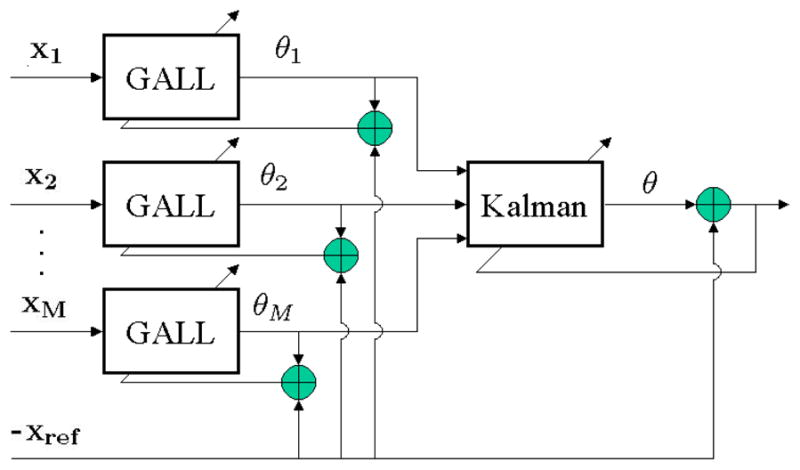
The overall estimation scheme consisted of two stages (Figure 1). In the first stage, M reconstruction signals, θm, were estimated from each of the M channels by using a bank of M GALL filters [3]. These M reconstructions were then linearly combined using a Kalman filter [5] to obtain the final reconstruction for that measurement, θ. Further detail of the algorithm can be obtained by studying the MATLAB code implementing the algorithm (available for free under the GPL [2] at http://www.physionet.org).
Figure 1.

Reconstruction Overview.
2.3. Individual reconstructions
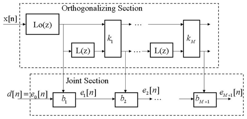
The GALL adaptive filter consists of orthogonalizing and joint sections (Figure 2), in which delays are replaced by Laguerre transfer functions
Figure 2.

GALL Overview.
| (6) |
and where the transfer function’s pole, a, is constant across the entire filter (note that for a = 0 the Laguerre transfer function becomes a simple unit delay). The input to the GALL filter was any of the M channels (with xT replaced by xTS), with the filter’s desired response set to xT.
The algorithm for training the GALL filter consisted of three major design parameters: P (the number of lattice stages), a (the pole location), and λ (the forgetting factor) [3, 5]. The number of lattice stages, P, was set to 35 and held fixed for all measurements and all signals. The specific value of P was chosen based on preliminary visual inspection of the maximum number of peaks in the spectra of a subset of the signals. The two other parameters, λ and a, were jointly optimized on a per signal, per record basis using the following cost function
| (7) |
where rmse(·, ·) is the root mean square error. The optimization function (7) was calculated over the penultimate 30 seconds (N – 2L ≤ n ≤ N – L) so that this optimization was performed individually over all 300 records. The optimization function (7) is related to the cost function (3), which was found to be, in general, the most stringent criterion of the two cost functions (3) and (4). Although the joint optimization of (7) was by far the most computational demanding aspect of the algorithm, it was implemented in a parallel fashion using an eight core 2.0 GHz multiprocessor machine (taking on average around 3 minutes per each 10 minute multi-channel record). In addition, (7) could possibly be modified for an online (recursive) implementation by tracking the minimum over a local area after an initial global search (or after some heuristic initialization).
After the GALL’s three major design parameters have been selected, the adaptive parameters of the filter (filter weights) were allowed to adapt to the desired response, xT. All of the filters’ adaptive parameters were frozen at n = N – L (last training sample) in order to generate the individual reconstructions for the missing section (N – L < n ≤ N).
2.4. Combined reconstructions
The second and final stage of the reconstruction algorithm consisted of combining the individual sample by sample reconstructions, θm[n], in order to generate an improved sample-by-sample final estimate of the missing signal, θ[n]. The M × N available reconstructions, Θ, were used as inputs to an unforced Kalman filter [5] where the vector of M × 1 weights, ẇ, was defined as the filter’s states
| (8) |
| (9) |
| (10) |
The weight updates of the Kalman filter were calculated using the simple set of equations
| (11) |
| (12) |
| (13) |
| (14) |
where λK is a forgetting factor between 0 and 1 for the Kalman filter, and K[n] is the M × M state error correlation matrix. The filter design parameter, λK, was determined by finding the optimal λK in similar fashion to the λ from the individual GALL reconstructions as described in the previous session. All of the Kalman filter’s adaptive weights were frozen at n = N – L (last training sample) in order to generate the final reconstruction for the missing section (N – L < n ≤ N).
3. Results
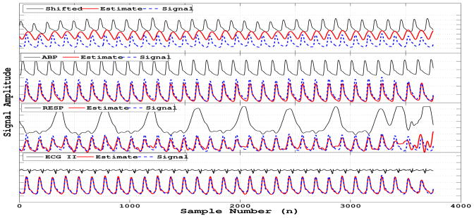
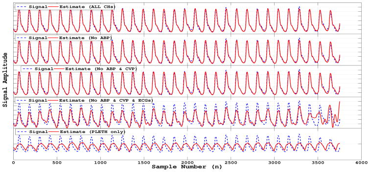
The algorithm results using the costs functions (3) and (4) are summarized on Table 1. Figures 3 and 4 show examples of the algorithm performance applied to a specific case where the signal to be reconstructed was a finger plethysmogram (PLETH) with the extra channels available being: arterial blood pressure (ABP), central venous pressure (CVP), respiration (RESP), electrocardiogram leads I, II and AVR (only ECG II is shown).
Table 1.
Scoring Results for the entire dataset
| Set A | Set B | Set C | Mean | |
|---|---|---|---|---|
| Q1 | 68.0 | 74.8 | 70.5 | 71.1 |
| Q2 | 80.9 | 84.9 | 84.0 | 83.2 |
| Mean | 74.5 | 79.9 | 77.7 |
Figure 3.
Example of individual reconstructions.
Figure 4.
Example of final reconstruction with degradation.
4. Discussion and conclusions
This paper describes an algorithm for estimating a missing channel from multiple concurrent signals using a combination of adaptive filters with forgetting factor to attempt to control for non-stationarities in the environment. The final score for the PhysioNet challenge was 0.71 (using Q1) and 0.83 (using Q2).
The algorithm described here can scale and shows signs of graceful degradation with respect to the number of channels being used. Significant improvements could be obtained by generating extra channels that incorporate any a priori knowledge of non-linear mapping among the original recordings. For instance, the estimation of the respiration signal may be improved by using an additional channel constructed from the ECG-Derived Respiration algorithm [4]. It is possible that the whole process may be implemented in an online recursive fashion after some initial optimization of the adaptive filters’ design parameters.
Acknowledgments
This work was funded in part by the National Institute of Biomedical Imaging and Bio- engineering and by the National Institute of General Medical Sciences, under NIH cooperative agreement U01-EB-008577 and NIH grant R01- EB001659. The author wishes to thank Daniel J. Scott, Joon Lee, and Roger Mark for providing assistance with the manuscript.
References
- 1.http://physionet.org/challenge/2010/
- 2.http://www.gnu.org/licenses/gpl.html
- 3.Fejzo Z, Lev-Ari L. Adaptive Laguerre-Lattice Filters. IEEE Transactions on Signal Processing. 1997;45(12):3006–3016. [Google Scholar]
- 4.Moody G, Mark R, Zoccola A, Mantero S. Derivation of Respiratory Signals from Multi-lead ECGs. Computers in Cardiology. 1985;12:113–116. [Google Scholar]
- 5.Haykin S. Adaptive Filter Theory. 4. Upper Sadle River, NJ: Prentice-Hall; 1990. [Google Scholar]


