Decision making under time pressure, modeled in a prospect theory framework

Abstract

The current research examines the effects of time pressure on decision behavior based on a prospect theory framework. In Experiments 1 and 2, participants estimated certainty equivalents for binary gains-only bets in the presence or absence of time pressure. In Experiment 3, participants assessed comparable bets that were framed as losses. Data were modeled to establish psychological mechanisms underlying decision behavior. In Experiments 1 and 2, time pressure led to increased risk attractiveness, but no significant differences emerged in either probability discriminability or outcome utility. In Experiment 3, time pressure reduced probability discriminability, which was coupled with severe risk-seeking behavior for both conditions in the domain of losses. No significant effects of control over outcomes were observed. Results provide qualified support for theories that suggest increased risk-seeking for gains under time pressure.

The goal of any decision maker is to make the most optimal decisions possible with a minimal amount of cognitive strain or effort. This may not be a very daunting task when given unlimited time to assess the decision problem, but many situations exist that require individuals to make decisions under deadlines. What happens to decision making in the presence of either potential gains or losses when we are under time pressure?

Prior approaches to time pressure and decision making

Much of the research that examines the effects of time pressure on decision making has found that a speed-accuracy tradeoff can occur with time constraints, and that individuals utilize many noncompensatory coping strategies, including acceleration and filtration of information (Janis, 1983; Miller, 1960; Payne, Bettman, & Luce, 1996; Svenson, Edland, & Slovic, 1990; Zakay, 1993). In the decision literature, noncompensatory decision strategies refer to heuristics that are characterized by a lack of complete relevant decisional information, and are therefore seen as less “rational” than compensatory decision strategies, which involve the use of all relevant aspects of options in the evaluation of choices. This finding has been corroborated in studies involving driving simulations (Stern, 1999) and emergency room decisions (Zakay, 1985). Other research examines the detrimental effects of time pressure on overall decision quality, with the general finding that individuals perform significantly worse under time pressure. This has been found in bet acceptance tasks (Payne, Bettman, & Johnson, 1988), in the accuracy of choice responses (Kocher & Sutter, 2006; Sutter, Kocher, & Strauβ, 2003), and in military attack simulations (Ahituv, Igbaria, & Sella, 1998). Furthermore, researchers have found an inverse relationship between the amount of time to deliberate on a decision and an individual’s confidence in that decision (Smith, Mitchell, & Beach, 1982).

This paper focuses on the effect of time pressure on individual choice behavior regarding risk. For studies such as this, participants are asked to make a choice between prospects, such as between a certain option and a risky option (Busemeyer, 1985) or between risky options of equal expected value but differing variances (Ben Zur & Breznitz, 1981; Bowman, Evans, & Turnbull, 2005). The effect of time pressure on preferential choice behavior is a topic of disagreement, with two alternative hypotheses in contention.

The first hypothesis claims that an inverse relationship exists between time pressure and one’s willingness to accept risk. Ben Zur and Breznitz (1981) asked participants to choose between two gambles that had comparable expected values but differed in either the gambles’ variances, the win and loss magnitudes, or the probabilities for a win. The amount of time constraint also differed between trials (low, medium, or high). Ben Zur and Breznitz reported that participants spent more time observing the negative elements of the prospects than the positive elements, and that, under high time pressure, they were less likely to accept riskier bets with high variances. The authors concluded that increases in time pressure lead to decreases in risk taking.

Other research, however, suggests that the relationship between time pressure and decision making is more complex. Busemeyer (1985) utilized a sequential-comparison approach (Busemeyer & Diederich, 2002; Busemeyer & Townsend, 1993) to investigate the effects of time pressure on preferential choice. The sequential-comparison model of preference proposes that an individual continuously makes comparisons among features of decision alternatives from moment to moment until one of the alternatives exceeds a given preference threshold, at which point that alternative is chosen. According to this approach, the magnitude of the decision threshold depends on the time to make a decision, so that increases in time pressure result in decreases in the threshold size. Busemeyer (1985) observed that when the variance between prospects was low, time pressure did not greatly influence decision behavior. However, when the risk was greater, a significant relationship emerged between time pressure and risk preferences; increases in time pressure led to greater risk taking for positive expected values (EVs) and greater risk aversion for negative EVs. These findings suggest that risk preference under time pressure may depend on the overall expected value among alternatives, whereby people are attracted to risks with positive expected value but averse to risks with negative expected value.

The effects of time pressure on individual choice behavior may take place through three mechanisms. First, individuals may perceive the marginal utility in potential gains and losses as altered when the risks are encountered in the presence of time stress than in the absence of time stress. Second, individuals may be more or less risk-seeking in the presence or absence of strict deadlines. Finally, under conditions of such pressure, individuals’ abilities to differentiate among probabilities may also change. Any of these means may lead to changes in overall choice behavior. Ben Zur and Breznitz’s (1981) model would predict decreases in risk acceptance with increases in time pressure, whereas Busemeyer (1985) suggests that individuals will be more attracted to risk under time pressure in a gain domain, albeit less so in a loss domain.

In the present study we also manipulated perceived control, as it is a variable that has proved relevant in recent models of decision making (Goodie, 2003; Goodie & Young, 2007). Developments in quantitative modeling have provided support for the argument that decisions based on objective prospects (which are classified within the domain of risk) can be adequately compared to decisions based on ambiguous prospects like confidence assessments (classified within the domain of uncertainty). Fox and Tversky (1998) formulated a two-step model of decision making under uncertainty that holds up well in comparison to similar estimations for risky prospects (also see Kilka & Weber, 2001). From these findings and our own recent work, the present research additionally aims to examine whether the relationship between time pressure and decision making is qualified by the type of decisions: decisions based on random events or decisions based on confidence in one’s knowledge.

Modeling decision behavior

This study utilized a framework of decision behavior based on prospect theory (PT; Kahneman & Tversky, 1979; Tversky & Kahneman, 1992), which takes into account the subjective value attributed to a given change in wealth (value function v) and the decision weight attached to the probability of a potential outcome (weighting function w). Maule and Svenson (1993) note the potential advantages in utilizing a PT framework to examine time pressure effects, suggesting that imposing a time limit would make the manifestation of the outcomes of a chosen prospect more immediate. This time limit would then affect the way in which a decision maker subjectively values the associated probabilities and outcomes. In this paradigm, individuals estimate certainty equivalents (CEs) for many binary bets under time pressure. We model a certainty equivalent (CE) value according to both the utility of the bet’s outcomes and the weighting of the bet’s probabilities. The formulation used in PT for this set of prospects is:

$$v(CE)=w(p)v(X)+\{1-w(p)\}v(Y),$$ (1)

where p represents the probability of a win, and X and Y equal the outcome of a win and loss, respectively, in a two-option bet. This formulation was previously employed by Young, Goodie, and Hall (2011).

The widely accepted value function v (Kahneman & Tversky, 1979),

$$v(X)=\theta X^{\alpha },$$

makes use of two parameters: θ is a scaling parameter, and α describes the degree of curvature in the value function (Figure 1a), representing the rate of change in the utility of gains depending upon the potential outcome’s relative distance from the individual’s reference point. This is accomplished mathematically by taking v to be a power function of the win outcome X.

Figure 1.

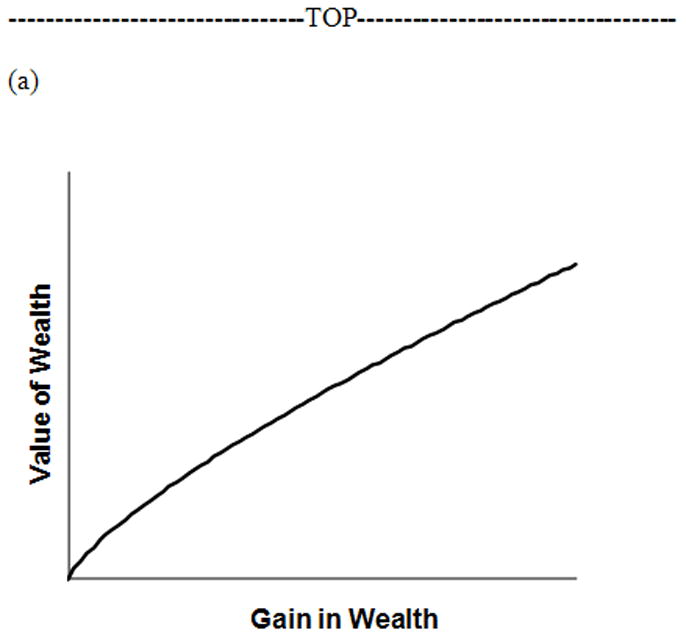
Typical prospect theory (a) value function with respect to gains and (b) probability weighting function.

We utilized Gonzalez and Wu’s (1999) specification of the probability weighting function w (Figure 1b), which applies to prospects in a gains-only framework, allowing for plausible psychological interpretations of the discriminability and attractiveness of probabilities:

$$w(p)=(\delta p\gamma )/\{\delta p\gamma +(1-p)\gamma \}.$$ (2)

In equation (2), γ represents probability discriminability (the curvature parameter) and δ represents probability attractiveness (the elevation parameter). An interpretation of decision behavior based on changes in γ and δ can be found in Young and colleagues (2011).

Utilizing statistical parameterization as defined by Gonzalez and Wu (1999) is particularly beneficial in the present case because of the inherent procedural similarities between their original design and that used in the current investigation. For example, following Gonzalez and Wu (1999), the current study utilized a gains-only or loss-only betting structure for gambles; additionally, the CE estimation procedures of both investigations are identical.

By substituting the specific forms given above for the value and weighting functions and applying the natural logarithm, we achieve a model of decision making suitable for nonlinear regression analysis:

$$log({\text{CE}}_{\mathit{ijk}})={{\alpha }_{ij}}^{-1}log[({X_{\mathit{ijk}}}^{{\alpha }_{ij}}-{Y_{\mathit{ijk}}}^{{\alpha }_{ij}})/\{1+{({\delta }_{ij}{O_{\mathit{ijk}}}^{{\gamma }_{ij}})}^{-1}\}+{Y_{\mathit{ijk}}}^{{\alpha }_{ij}}]+e_{\mathit{ijk}},$$ (3)

where CE_ijk denotes the CE elicited on the kth bet given to the jth subject in the ith experimental condition, and O_ijk = p_ijk/(1 − p_ijk) denotes the odds of winning.

Modeling each participant’s data within the PT framework permits analysis of time pressure effects on three unique aspects of risk taking. Differences in α between groups would refer to the way possible gains in wealth are valued, whereas differences in γ would indicate differentially nonlinear weighting of probabilities and differences in δ would imply differences in the overall attractiveness of risk.

The Present Research

Using these methods, we sought to rigorously test the two current theories of the impact of time pressure on decision making: that time pressure leads to a decrease in overall risk taking (Ben Zur & Breznitz, 1981; Smith et al., 1982), and that time pressure has a differential effect on decision behavior, leading to an increase in risk taking when expected value of prospects is positive, but a decrease in risk taking when the expected value is negative (Busemeyer, 1985; Busemeyer & Diederich, 2002).

Gonzalez and Wu’s (1999) conception of PT’s probability weighting function postulates that the δ parameter, which drives the elevation of the 2-parameter weighting function, reflects how much an individual finds a gamble or risk to be attractive. As such, increases or decreases in δ represent increases or decreases in overall risk taking, respectively. Consequently, we proposed two alternative hypotheses based on the competing theories presented above.

1. Time pressure will lead to a decrease in the overall attractiveness of risk, as evidenced by significantly smaller δ parameter values for those estimating CEs under time pressure for both gains and losses.

2. Time pressure will lead to an increase in the overall attractiveness of risk in the presence of gains, as evidenced by significantly larger δ parameter values for those estimating CEs under time pressure in the domain of gains. Furthermore, time pressure will lead to a decrease in the overall attractiveness of risk in the presence of losses, which will result in smaller δ parameter values when making decisions under time pressure.

These two competing hypotheses were tested in three experiments; some participants were given unlimited time to estimate CEs for various bets, while others were required to estimate CEs for bets under time pressure. In the first two experiments, bets were framed in a gains-only structure so as to yield positive expected values; in the third experiment, bets were framed in a loss-only structure to yield negative expected values.

EXPERIMENT 1

In Experiment 1 we assessed whether participants showed differences under time pressure in the nonlinearity of value functions, probability discriminability, or overall risk attractiveness in a two-factor, between-subjects design. Participants were randomly assigned to encounter gains-only bets in either a Time Pressure condition or a No Time Pressure condition. In order to assess whether decision type may have a differential effect on decision behavior, we included a bet-type factor into the design as well; participants encountered bets based on either random lotteries (“Random” condition) or the correctness of their answers to questions that asked for binary comparisons of US state populations (“Knowledge” condition). A modified Georgia Gambling Task (GGT; Goodie, 2003; Young et al., 2011) was utilized in the present experiments to allow for the estimation of CEs for each bet. All bets were constructed to be fair, meaning the average value of betting on their answers was equal to the value of rejecting the bet, if a participant’s confidence was well-calibrated to his or her accuracy. This design allowed us to model the weighting function across half of the probability spectrum, .51–.99. This experiment utilized 7 confidence categories and 15 possible win-loss amounts, yielding up to 105 bets for each participant.

As one means of enhancing motivation, Experiment 1 gave participants the opportunity to play out one of their bets for real money.

Method

Participants and materials

Participants were 101 volunteers (65 female) who were recruited from the Research Pool of the Psychology Department at the University of Georgia in exchange for partial psychology course credit. Up to three participants at a time worked at individual computer workstations. Those who had previously participated in related experiments were excluded. Participants had the opportunity to play out one of their bets for real money (1/5 face value of the bet) at the end of the session.

Procedure

For Phase 1, all participants answered questions about U.S. state populations and assessed their confidence in each answer. The first question asked participants to make a binary forced-choice comparison of the populations of two randomly-chosen U.S. states. The following is an example state population question that a participant might have encountered.

Which state has the higher population according to the U.S. Census bureau estimates for 2005:
New Jersey	Illinois

The second question type asked participants to assess their confidence in each answer based on one of the following seven categories: 51%, 55%, 65%, 75%, 85%, 95%, and 99%. Participants answered 100 U.S. state population questions of this type. In the process of answering all 100 general knowledge questions, a participant would likely express, for example, 75% confidence in multiple answers. Because a participant may not feel exactly 75% confident in all of those answers, the last portion of Phase 1 displayed up to 5 of the participant’s 75% confidence answers and asked the participant to choose among those options one answer that best exemplified an answer in which he/she was 75% confident. This same process was followed for all confidence categories that had been used more than one time.

In Phase 2, all participants encountered as many as 105 unique bets. Participants in the Knowledge conditions encountered bets based on their answers to the U.S. state population questions, whereas participants in the Random conditions encountered bets based on random probabilities. The task for all participants was to estimate a CE for each bet; a CE is a dollar amount that, if provided with certainty, the participant views as equivalent in subjective value to a bet.

Although the surface features of the Knowledge and Random wagers were different, the underlying structure of these bets was identical. The bets were obtained by crossing the seven probability levels used in the confidence estimation portion of Phase 1 with 15 win-loss amounts. The win-loss amounts adopted from Gonzalez and Wu (1999) were as follows (in dollars): 25-0, 50-0, 75-0, 100-0, 150-0, 200-0, 400-0, 800-0, 50-25, 75-50, 100-50, 150-50, 150-100, 200-100, 200-150. This paradigm incorporated only gains-only trials; a “loss” consists of either no change in wealth, or an absolute gain, which is a loss only in the sense of being a smaller gain. Each bet displayed the amount of money gained for a win, the amount of money gained for a loss, and either the answer given in Phase 1 (for the Knowledge condition) or the probability of a random-chance win (for the Random condition) in the event of accepting the bet.

For the Knowledge condition, the outcomes were determined by the correctness of participants’ answers to the U.S. state population questions; correct answers resulted in a win, and incorrect answers resulted in a loss. For the Random condition, the outcome of each wager was determined by a random gamble in which the probability of winning was matched to one of the seven confidence categories used in Phase 1. Participants in all conditions estimated CEs to the nearest dollar using the same narrowing-down process as Gonzalez and Wu (1999). An example of the narrowing-down process is illustrated in Figure 2.

Figure 2.

A hypothetical example of the narrowing-down process for CE estimation for a bet in the Knowledge condition, which indicates that the participant believed Illinois has a higher population than Ohio. If correct, the participant would win $25 in this bet. The figure describes both the first screen in the narrowing process and the last screen. Here, the participant estimated a CE of $17 for this bet.

To ensure that participants understood the gambling task, they completed an informal training session with an experimenter prior to beginning the computer-driven study. This training session allowed the participants to experience example trials of the task so that participants could learn what the gambling task required of them and understand how deliberately under- or overestimating a CE for any gamble would be disadvantageous if that gamble were to be played out for real money at the end of the study session. Experimenters requested that participants think through each wager as if the wagers could be played out at full face value.

At the beginning of Phase 2, Knowledge and Random participants were randomly assigned to one of the two time pressure conditions. Those assigned to the No Time Pressure condition were given an unlimited amount of time to estimate CEs for each bet. Participants assigned to the Time Pressure condition were informed prior to beginning the betting task that they would only be given 10 seconds on the first bet screen of the narrowing-down process and 5 seconds for every subsequent screen. If a Time Pressure participant exceeded any time limit within a bet, she or he was notified of the time limit violation and told that that bet would not be played out for real money if selected at random at the end of the session.

Modeling

We modeled subject specific parameters via mixed effects: α_ij = α_i0 +a_ij, γ_ij = γ_i0 + c_ij, δ_ij = δ_i0 + d_ij, where α_i0, γ_ij, δ_i0, i =1,…,4 are fixed population-level parameters, and a_ij, c_ij, d_ij are subject-specific random effects assumed to jointly follow a multivariate normal distribution with zero mean and variance-covariance matrix Φ. Random subject effects are assumed independent across subjects and independent of model errors e_ij =(e_ij1,…,e_ijnij)′, which are assumed multivariate normal with mean zero and variance-covariance matrix Σ_ij. To account for non-constant variance and correlation observed in the data, the within-subject error variance-covariance matrix Σ_ij was modeled with an AR(1) correlation structure (autoregressive of order 1; Pinheiro & Bates, 2000), and, because of much greater observed variability for bets involving a zero loss amount, two distinct error variance parameters depending upon whether X_ijk =0. This model is an example of a nonlinear mixed-effects model; for more on this class of models, their use in modeling repeated measures data like those from the current experiments, and statistical methods of estimation and inference in this class using the S-PLUS nlme library, see Pinheiro and Bates (2000).

Results and Discussion

Participants may fail to follow basic laws of consistency, dominance, or transitivity, for example if a participant that views a gamble with p(win)=.51 as more attractive than the same gamble outcomes with p(win)=.99, due to inattention during the task. If a participant demonstrated a clear lack of internal consistency in these terms, the participant was removed from analysis. Based on these violations, we removed 2 participants from the Knowledge-No Time Pressure condition prior to analysis.

Basic confidence calibration statistics were compared between Random and Knowledge conditions to examine whether individuals showed qualitatively different levels of over- or under-confidence in their answers to the U.S. state population questions. Overall overconfidence rates, which were found by subtracting overall accuracy rates from overall confidence rates, were found not to differ significantly between the Random (−.0042; SD = .103) and Knowledge conditions (.0041; SD = .098; t(92) = 0.398, p=.692), indicating that participants in both conditions had approximately the same rates of confidence for their answers to the state population questions.

To assess whether the time limits imposed upon Time Pressure participants caused participants to evaluate all bets more quickly than No Time Pressure participants, average bet screen times were computed for all participants. As predicted, Time Pressure participants spent significantly less time (3.28 seconds; SD = 1.03) evaluating gambles and estimating the first CE options for every gamble than those who had no time limits (6.26; SD = 2.45). These differences were statistically significant, even after allowing for different variances in the two groups, which were found to differ significantly according to Levene’s test (t(92.442) = 7.814, p<.01). Furthermore, we examined the proportion of Time Pressure participants’ bets that exceeded the time limits. Out of the 105 possible bets, participants in the Time Pressure condition violated the time limits on an average of 2.76 bets. Also, over half of these time limit violations occurred within the first 10 gambles of the experiment session. Based on these findings, participants appeared to learn very quickly to process the gamble information at a fast rate. The relatively good model fit for the gambles that did not violate the time limits suggests that the time constraints created a stressed environment without being so constricting as to cause a decisional “melt-down” for participants.

We computed results by analyzing participant CE data using the nonlinear mixed effect model (Equation 3), which allows distinct parameters by treatment for both the generally accepted value function (α) and the Gonzalez and Wu (1999) probability weighting function (γ and δ).

Final subjects per condition, means and standard errors of estimated δ, γ and α, parameter values are shown in Table 1. In this two-factor study, we found no interaction effects between the Time Pressure and Bet-Type factors. The presence of time pressure had a significant positive effect on δ (F(1,10015) = 4.07, p<.05¹). This increase in the attractiveness of risk exists just as strikingly even if the Knowledge conditions are removed from analysis (Time Pressure-Random = 1.687; No Time Pressure-Random = 1.397). Thus we conclude that this increase in δ is pervasive. This result clearly suggests that, under time pressure, individuals perceive risk as significantly more attractive across the upper half of the probability spectrum than under situations in which no time pressure is felt. Differences in estimated γ values were not statistically significant across the Time Pressure and No Time Pressure conditions (F(1,10015) = 0.78, p=.38). This lack of change in probability discriminability (.436; .497) also exists for Random bets in isolation. Figure 3a presents partial weighting functions utilizing γ and δ parameter estimates from both conditions, with extensions depicted from the observed probability range of [0.5,1.0] to the full range. Differences in α parameter estimates were also not statistically significant between the Time Pressure conditions (F(1,10015) = .007, p=.94), which are depicted graphically in Figure 3b, suggesting no effect of time pressure on the utility of gains. Again, the marginal utility of gains for Random bets does not change in the presence (.965) or absence (.966) of time pressure.

Table 1.

Sample sizes, means and standard errors for all conditions in Experiment 1.

	Time Pressure		No Time Pressure
	Knowledge (n=25)	Random (n=26)	Knowledge (n=20)	Random (n=27)
δ estimates	1.533 (.202)	1.687 (.201)	1.009 (.212)	1.397 (.191)
γ estimates	.718 (.069)	.436 (.063)	.774 (.072)	.497 (.061)
α estimates	.899 (.072)	.965 (.072)	.910 (.075)	.966 (.068)
Marginal Means for Time Pressure Factor	δ = 1.610 (.142) γ = .577 (.0466) α = .932 (.0506)		δ = 1.203 (.143) γ= .636 (.0472) α = .938 (.0506)

Figure 3.

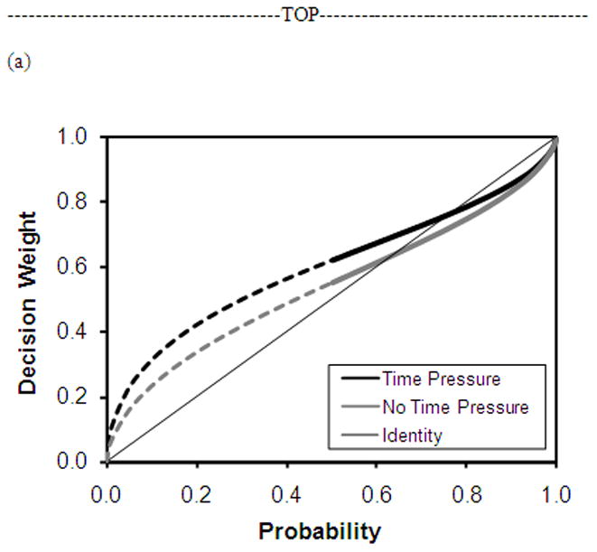
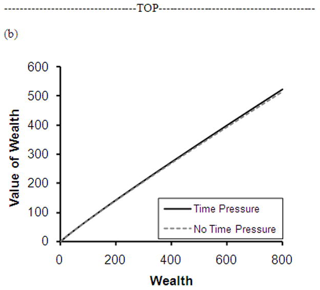
Experiment 1 results for (a) probability weighting function curves and (b) value function curves observed for main effect of Time Pressure. Solid lines in the weighting function curves represent the observed range of probabilities, and dotted lines represent an extension to the full probability spectrum.

The magnitudes of our observed δ values are larger than the medians reported by Gonzalez and Wu (1999), but are not outside the previously reported range. Young, Goodie, and Hall (2011), for instance, reported δ values greater than 1.0 in multiple experiments, suggesting a weighting function that describes high attractiveness to risk. Gonzalez and Wu’s participants showed considerable variability in individual shapes of the weighting functions, with δ magnitudes ranging between 0.21 and 1.51. In fact, the weighting functions of 4 of their 10 subjects evidenced trends towards what the authors called supercertainty, or increased probabilistic risk attractiveness.

The significant increase in δ for all bets in the Time Pressure condition provides support for a positive impact of time pressure on the overall attractiveness of risk, Hypothesis #2. These results support the findings of Busemeyer (1985), which suggested an increase in risk taking in the domain of gains under time pressure.

EXPERIMENT 2

Experiment 1 utilized bets based on binary forced-choice comparisons of state population. The least confidence that a decision maker can have in an answer to a binary comparison is .50. As such, the resulting responses can only be modeled with respect to half of PT’s probability weighting function. Further, low-probability events are of considerable interest in the decision literature. In order to examine decision behavior in a more comprehensive manner, Experiment 2 was constructed to allow for the estimation of probability weighting functions that take into account a larger range of the probability spectrum.

This was accomplished by having participants estimate CEs for bets with p(win) amounts less than .50, with the primary change being to ask which of six states has the greatest population, as opposed to identifying the greatest population out of only two states. As in Experiment 1, we assessed whether participants evidenced a difference in decision making behavior under time pressure in the nonlinearity of their value functions, the discriminability of probabilities, or the attractiveness of risk. Also as in Experiment 1, this two-factor between-subjects design randomly assigned participants to one of four conditions: Time Pressure-Knowledge, Time Pressure-Random, No Time Pressure-Knowledge, and No Time Pressure-Random. The modified Georgia Gambling Task was again utilized to model decision behavior and estimate parameter values of δ, γ and α for each condition. Thus, Experiment 2’s design allowed an examination of how individuals assess bets with prospects that are either likely (greater than 50% chance of winning) or less than likely (less than 50% chance of winning). Participants encountered bets on either random events or their answers to general knowledge questions in a way that allowed for us to model the probability weighting function across a larger range of the probability scale. This experiment utilized 6 confidence categories and 12 possible win-loss amounts, yielding up to 72 bets for all participants.

Method

Participants and materials

Eighty-five new undergraduate participants (53 female) were recruited for Experiment 2 from the same population as Experiment 1. Participants were run up to three-at-a-time at personal computer workstations. Those who had previously participated in related experiments were excluded.

Procedure

In Phase 1, participants answered general knowledge questions and assessed their confidence in each answer. For every question, participants were asked to choose which of six randomly-chosen U.S. states had the highest population, for example:

Which of the following six U.S. states has the highest population, according to the 2005 U.S. Census Bureau:
Arizona	Michigan	Texas	Rhode Island	Idaho	Oregon

For questions of this type, a pure guess would induce approximately 17% confidence in any answer. The second question in Phase 1 asked participants to assess their confidence in each of their answers with one of the following six categories: 20%, 35%, 50%, 65%, 80%, and 95%; these confidence categories allow for a relatively proportional division of the range of possible probabilities. Participants responded to 100 state population questions in this way. As in Experiment 1, each participant chose one answer that best exemplified an answer in which he/she felt each of the 6 stated degrees of confidence.

In Phase 2, participants encountered one of two types of bets: those based on their answers to the U.S. state population questions or those based on random lotteries. Participants estimated CE estimates for up to 72 bets. The 72 bets were obtained by crossing the six probability levels with 12 of the 15 win-loss amounts previously utilized: [25-0, 50-0, 100-0, 150-0, 200-0, 400-0, 800-0, 50-25, 75-50, 100-50, 150-100, 200-150]. For those in the Knowledge conditions, the outcomes depended on the correctness of their answers to the U.S. state population questions. The same CE estimation process was used as in the previous experiment. Those in the Time Pressure conditions were allotted 10 seconds to assess the first screen for each bet and 5 seconds for every subsequent screen. The No Time Pressure conditions had no time limits on any bet screens. Although participants in Experiment 2 were not able to play out any of their bets for real money at the end of the study, the experimenters requested that all participants think through each wager as if it could be played out at full face value.

Results and Discussion

We removed data from 1 participant from the Time Pressure-Knowledge condition prior to analysis due to internal inconsistency. For Time Pressure participants, the number of time limit violations (M = 5.24) was higher than those found in Experiment 1 (M = 2.76), however the average proportion of viable gambles per participant remained high (.92). This suggests that, although participants without money incentives may not stay within the time constraints as much as those with real money incentives, participants are still highly motivated to complete the gambling tasks within the time limits.

The form of the nonlinear mixed effects model fit to the data and on which statistical inference was based was the same as for Experiment 1.

Refer to Table 2 for Experiment 2 sample sizes, means, and standard errors for the estimated δ, γ and α parameter values. For this set of data, we compared CE responses from both Time Pressure conditions to those from the No Time Pressure conditions. The significant main effect of Time Pressure on δ indicates that overall risk attractiveness across Time Pressure conditions was significantly greater than that across the No Time Pressure conditions (F(1,5170)=5.023, p<.05). We found no main effect of Time Pressure on estimated γ values (F(1,5170)=1.639, p=.20) or on estimated α values (F(1,5170)=0.006, p=.94). Simple effects tests revealed that the main effect of Time Pressure on δ was driven mainly by the Random conditions’ differences; Random participants under time pressure yielded significantly higher estimated δ values than their no time pressure counterparts (F(1,5170)=3.894, p<.05). This simple effect of Time Pressure on estimated δ values was not found within the Knowledge domain (F(1,5170)=1.489, p=.22). One unexpected result in Experiment 2 was a higher estimated γ value in the Random domain when participants were not under time pressure than when they were (F(1,5170)=4.824, p<.05), leading to a weighting function with a smaller degree of curvature when not under time pressure. This result may suggest that individuals discriminate among probabilities in a more linear fashion when the bets under consideration are based on random events and when the decisions can be made without time stress. With more experience with these bets, individuals may have been indirectly trained to form more accurate perceptions of the probabilities associated with those decisions when given unlimited time to make those decisions. However, as this increase in the linearity of the probability weighting curve was not found for the Random-No Time Pressure condition in Experiment 1, we do not speculate on other theoretical explanations. No other simple effects were statistically significant.

Table 2.

Sample sizes, means, and standard errors for all conditions in Experiment 2.

	Time Pressure		No Time Pressure
	Knowledge (n=19)	Random (n=22)	Knowledge (n=21)	Random (n=22)
δ estimates	1.622 (.183)	1.634 (.169)	1.321 (.166)	1.176 (.160)
γ estimates	.547 (.088)	.458 (.080)	.508 (.083)	.711 (.083)
α estimates	.899 (.078)	.900 (.074)	.903 (.072)	.907 (.069)
Marginal Means for Time Pressure Factor	δ = 1.627 (.124) γ = .502 (.0595) α = .900 (.0535)		δ = 1.248 (.115) γ= .609 (.0584) α = .905 (.0499)

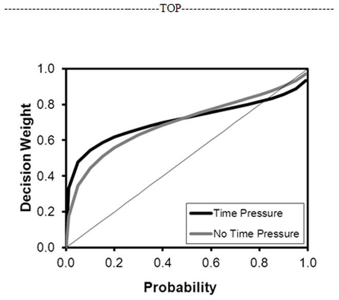
Observed weighting functions and value functions for both conditions are depicted in Figures 4a and 4b, respectively. CE responses from participants in the Time Pressure conditions yielded a weighting function with a significantly higher estimated δ value than CE responses from those in the No Time Pressure conditions, supporting an overall increase in risk attractiveness when betting on events under time pressure.

Figure 4.

Experiment 2 results for (a) probability weighting function curves and (b) value function curves observed for main effect of Time Pressure.

Post hoc two-way interaction tests revealed no significant gender differences in observed δ values in the presence or absence of time pressure data. Significant differences in observed δ values were not found for either the time pressure-by-gender interaction or the main effect of gender.

EXPERIMENT 3

As Experiments 1 and 2 focused on gambles that incorporated only potential gains, we ventured to examine the effects of time pressure when the gambles presented potential losses. A large body of research argues for the use of distinct utility functions for losses and gains. Specifically, in situations that incorporate pure losses (non-mixed gamble settings), individuals systematically demonstrate severe loss aversion, which implies that losses are weighted more than, and in some cases up to twice as strongly as, equivalent gains (e.g., Kahneman, Knetsch, & Thaler, 1990; Tversky & Kahneman, 1991; Tversky & Kahneman, 1992; Wehrung, 1989).

As the results of Experiments 1 and 2 did not reveal differences based on bet type, all Experiment 3 participants assessed CEs on Random bets and were assigned to either Time Pressure or No Time Pressure conditions. Consequently, only Phase 2 of the original task was implemented. In many ways, many elements of the Experiment 3 paradigm were the same as those used in Experiments 1 and 2: participants in this between-subjects design estimated certainty equivalents for 84 unique bets using the modified GGT, and half of the participants made these choices under time constraints. The unique contribution to this study lay in the fact that all potential outcomes in the wagers were framed as potential losses rather than gains.

Method

Participants and materials

Eighty-four new undergraduate participants (67 female; Time Pressure = 42) were recruited for Experiment 3 from the same population as Experiments 1 and 2 and were run up to three-at-a-time at personal computer workstations.

Procedure

After random assignment to either the Time Pressure or No Time Pressure condition, participants estimated CEs for 84 random lottery bets. These bets were obtained by crossing seven probability levels (.01, .10, .30, .50, .70, .90, and .99) with 12 large loss-small loss amounts (25-0, 50-0, 100-0, 150-0, 200-0, 400-0, 800-0, 50-25, 75-50, 100-50, 150-100, and 200-150). Although the same CE estimation process was used as in the previous experiments, participants were now encountering loss-only risks and estimating the largest amount of money they would be willing to pay in order to avoid taking the risk (which may lead to the large loss). An example of an Experiment 3 trial is below:

For the gamble now under consideration:
Large loss amount:	$100
Small loss amount:	$0
Probability of large loss:	90%
What is the largest amount of money you would be willing to pay in order to avoid taking the risk?

The Time Pressure condition had a 10-second limit for the first screen of each bet and a 5-second limit for every subsequent narrowing-down screen, while the No Time Pressure condition had no such time limits. As in Experiment 1, participants in Experiment 3 played one of their bets out for real money at the end of the experiment session. In order to allow participants to potentially “lose” money, participants were first shown several cash envelopes which represented the modest cash incentives for the gambles (1/10 face value of the larger loss amounts for each bet type) at the beginning of the experiment session. Participants were endowed the cash envelope that matched their randomly-chosen gamble (between $5 - $80) once they completed the entire gambling task. Then, the outcome for that gamble was determined utilizing a computerized random number generator function, and participants were required to give back the appropriate amount of that endowment depending upon the outcome of the gamble. As in previous experiments, participants were encouraged to think through each wager as if it were going to be played out for real money at full face value.

Results and Discussion

As was found in Experiment 1, Time Pressure participants spent significantly less time (3.62 seconds; SD = 1.00) evaluating the first CE estimation screen for each gamble than those who had no time limits (7.57; SD = 2.59), supporting the view that the time pressure manipulation was effective in requiring participants to evaluate gambles at a faster rate (t(54.53) = 9.321, p<.01). Time Pressure participants violated the time limits an average of 2.57 out of 84 gambles, indicating that approximately 97% of the gambles were completed appropriately within the time limits. As found in Experiment 2, participants under time pressure were highly motivated to complete the gambling tasks within the time restrictions.

The nonlinear mixed effect model used on Experiments 1 and 2 was again fit to the CE data. One major difference in the model-fitting for this experiment was that previously-estimated win amounts were now defined as “large loss” amounts, and previously-estimated loss amounts were defined as “small loss” amounts. As such, if participant A were to provide a CE of $75 to the bet above while participant B were to estimate a CE of $94, A would be seen as more risk-seeking than B.

In the loss domain, time pressure had an impairing effect on Time Pressure participants’ abilities to discriminate among probabilities, which is reflected in significantly lower observed γ values. Data from our sample revealed no significant group-level differences in either risk attractiveness (δ) or the utility of potential losses (α) as a function of time pressure (see Table 3). This pattern of findings can be seen in Figure 5. It is also striking that both conditions’ observed probability weighting functions indicate extremely risk-seeking attitudes. Estimated δ parameter values exceed 2.6 in both the Time Pressure and No Time Pressure conditions, and the curves in Figure 5 are predominantly above the positive diagonal, reflecting extreme willingness to accept risk in lieu of buying out of a gamble. Indeed, 5.2% of all CEs reflected certainty equivalents of $0. This reflects extreme risk seeking among this subset of choices and suggests that limiting our CEs to whole dollar values may not have permitted measurement of CEs less than $1.

Table 3.

Sample sizes, means, and standard errors for both conditions in Experiment 3.

	Time Pressure (n=42)	No Time Pressure (n=43)
δ estimates	2.679 (.050)	2.713 (.049)
γ estimates	0.366 (.042)	0.555 (.043)
α estimates	1.205 (.086)	1.267 (.085)

Figure 5.

Experiment 3 results for probability weighting function curves observed for main effect of Time Pressure.

We tested possible effects of gender on observed parameter values with and without time pressure via two-way interaction tests. No significant differences emerged in observed α, γ, or δ parameter values for either the main effect of gender or the Time Pressure-by-Gender interaction, although the uneven gender distribution in this data set may dampen the validity of this result.

The heightened risk seeking in the loss domain is conceptually consistent with the prior empirical literature (Kahneman & Tversky, 1979; Tversky & Kahneman, 1992), marking a further step forward in modeling the thorny loss domain in a quantitatively sophisticated manner (e.g., Abdellaoui, 2000; Abdellaoui, Bleichrodt, & L’Haridon, 2008; Bruhin, Fehr-Duda, & Epper, 2010). The extreme risk-seeking behavior found in this study, reflected as elevated probability weighting curves in both conditions, may reflect the impact of a ceiling effect that impedes the detection of an effect of time pressure on risk attractiveness in the loss domain.

GENERAL DISCUSSION

In three experiments we examined the effects of time pressure on decision behavior, formally modeling responses within a prospect theory framework that allows for a rigorous and psychologically-relevant explanation of systematic fluctuations in risk taking. Participants answered general knowledge questions, assessed their confidence in all answers, and estimated certainty equivalents for bets – some based on their answers to the general knowledge questions, and others on a random lottery. Some participants assessed CEs under time pressure, while others were given no time limits. Results from two studies consistently demonstrated more elevated weighting functions for decision makers in the Time Pressure conditions when the gambles incorporated gains-only outcomes, suggesting a significant increase in the overall attractiveness of risk when making decisions under time pressure in a gain domain. A third study explored the effect of time pressure on risk attractiveness in a loss domain, and any such effect of time pressure on risk attractiveness appears to have been overshadowed by extreme risk seeking, which is consistent with the prior literature, at least in a qualitative sense. Instead, participants who encountered gambles under time pressure failed to discriminate among probabilities as well as those without time pressure.

In Experiment 1 participants estimated CEs for bets that had greater-than-even odds of success either under time pressure or under no time pressure. Modeling results indicated that time pressure leads to increased risk attractiveness, as evidenced by significantly higher δ parameter values for the probability weighting function in the Time Pressure conditions relative to the No Time Pressure conditions. In Experiment 2, this trend was extended to a broader portion of the probability spectrum, validating that the overweighting of probabilities under time pressure pervades a wide range of the probability spectrum. The trend was also extended to designs that utilize hypothetical incentives rather than real monetary incentives. Operating in the loss domain, Experiment 3 required participants to estimate the amount of money they were willing to pay to avoid the risk of hypothetical losses. In addition to the finding that time pressure diminishes probability sensitivity, the large observed magnitudes for δ suggest that the loss domain invokes acute and pervasive risk-seeking behavior. A ceiling effect of risk seeking may have inhibited the ability to observe an effect of time pressure on risk attractiveness in the presence of losses. However, the time pressure manipulation had a debilitating effect on probability discriminability, as can be seen in significantly lower observed γ values for the Time Pressure condition.

These results suggest that time pressure has a straightforward effect in making individuals more risk seeking in the gain domain and impedes probability discriminability in the loss domain. Further, by modeling CEs in a formal prospect theory framework, we can assess decision making under time pressure more rigorously than had previously been done. In modeling both probability weighting functions and value functions across groups, we demonstrate that time pressure leads to an increase in overall risk attractiveness across much of the probability spectrum when assessing potential gains.

Increased attractiveness of risk for gains under time pressure

These results align well with previous research that purports increased risk taking for decisions under time pressure when overall expected value of prospects is positive (Busemeyer, 1985). Busemeyer’s examination of the effects of time pressure on preferential choice behavior suggested a more complex relationship that had previously been implied. Specifically, when participants choose between certain and risky prospects involving potential gains, increases in time pressure lead to increases in risk taking in the form of greater acceptance of the risky prospect. This effect was specifically found for decision making scenarios with positive expected value, while the opposite effect – greater risk aversion in the form of greater acceptance of the certain prospect – was found for scenarios with negative expected value.

This in some ways supports Busemeyer’s (1985; Busemeyer & Diederich, 2002) account for this increase in risk taking for prospects with positive expected value; individuals may utilize a sequential comparison approach toward risk preferences, under which comparisons are made between the various attributes of prospects over time in order of attribute importance. However, this support is attenuated by the absence of an observed effect of time pressure in the domain of losses. We propose that Busemeyer’s theory, originally advanced to explain preferential choice behavior, can also be applied to individual choice behavior involving the elements of prospect theory.

Decreased probability discriminability among potential losses under time pressure

It is possible that the significant effect of time pressure on probability discriminability in the loss domain complements aspects of Busemeyer’s claims as well. According to all accounts of probability discriminability, individuals can appreciate an increase in probability at very high and very low levels.

In the present context, participants under time pressure have less time available to evaluate probabilities. Applied to Busemeyer’s (1985) concepts, time pressure may lower the threshold bound that individuals set to weigh the probability associated with the larger loss, leading people to evaluate probabilities in a way that suggests a step function rather than a more linear function. With a step function, sensitivity to probability changes occurs only near the endpoints, whereas the probabilities within the middle range are discriminated with less scrutiny. The step function may serve an adaptive purpose under some circumstances by simplifying the task when the environmental characteristics so dictate.

Implications for time pressure research and applied settings

Decision researchers have attempted to explain decision making under experienced stress and conflict using various theoretical and methodological approaches, including individual judgment, choice, and processing strategy. The present findings provide a new approach to investigating time pressure effects on decision making, examining fluctuations in risk taking behavior, directly due to time pressure, through three psychologically relevant components of prospect theory: probability attractiveness, probability discriminability, and the utility of potential monetary outcomes. Previous time pressure research, which generally examined bet acceptance rates or confidence in bet acceptance, provided less rigorous assessment of choice behavior. The unique contribution of time pressure to decision making has important theoretical implications, suggesting that an individual’s perception of risk attractiveness may increase when required to make decisions under time stress.

Researchers in many applied settings have an interest in how individuals perform under stressful environments and emergency situations such as military command decisions, fire emergencies, and aviation (Flin, Salas, Strub, & Martin, 1997). Time pressure research plays a central role in such settings, and the present findings provide a significant contribution to the ever-growing understanding of how humans navigate through everyday decision making in a variety of contexts.

Limitations

One limitation of the present research concerns the hypothetical nature of the gambles that participants encountered in Experiment 2. Taken as a whole, we followed the advice of Hertwig and Ortmann (2001) that both hypothetical stakes and real money incentives should be taken into account; real money incentives were utilized for Experiments 1 and 3, and we provided only hypothetical monetary incentives for Experiment 2. In that our group-level estimated parameters for both experiments are similar, the present results provide further evidence that performance in this type of task may be equivalent in the presence of both real and hypothetical monetary incentives.

A second limitation of this research concerns the nature of the matching procedure in this design. While Busemeyer (1985) and Ben Zur and Breznitz (1981) used direct choice procedures to elicit preferences from participants, the present study required participants to choose from among a variety of response options. It is possible that this inconsistency in task procedures may have produced changes in preferences simply because the procedure invariance principle was violated (see Fischer, Carmon, Ariely, & Zauberman, 1999). As such, the present findings may be restricted to decisional scenarios in which possible preferences are made by choosing from an array of options.

In addition, although the overall parameter estimates for δ (overall risk attractiveness) in these studies are within the previously-reported range of possible estimates, they are generally greater than those reported by Gonzalez and Wu (1999) and Tversky and Kahneman (1992). These δ estimates may be a function of a number of factors, including the presence of other participants and the researcher in the same computer lab suite. Due to time and space constraints, all experiments in the present study were conducted in a 3-workstation lab suite that allowed the researcher to run up to three participants at once. This could have added social pressure to the intended time pressure. The “risky shift” (Vinokur, 1971) may be playing a role in elevating participants’ willingness to accept risk, even in the absence of sanctioned contact with those in the room.

Conclusion

The prior literature on decision making under time pressure provided diverging accounts, with one line of research suggesting that time pressure leads to decreased risk-taking, and the other line suggesting that time pressure leads to an increase in risk-seeking for gains but a decrease in risk-seeking for losses. In three studies, we utilized a sophisticated, prospect theory-based computational model to investigate the effects of time pressure on risk-taking. Here, time pressure led to increased risk attractiveness in a gain domain and decreased probability discriminability in a loss domain. These findings point to multiple cognitive processes involved in decision making that may be differentially influenced by time pressure.

• Prospect theory-based modeling of decision making under time pressure

• Certainty equivalents were estimated for bets framed as either gains or losses.

• Time pressure increased risk attractiveness for gains.

• Time pressure reduced probability discriminability for losses.

References

- Abdellaoui M. Parameter-free elicitation of utility and probability weighting functions. Management Science. 2000;46:1497–1512. [Google Scholar]
- Abdellaoui M, Bleichrodt H, L’Haridon O. A tractable method to measure utility and loss aversion under prospect theory. Journal of Risk and Uncertainty. 2008;36:245–266. [Google Scholar]
- Ahituv N, Igbaria M, Sella A. The effects of time pressure and completeness of information on decision making. Journal of Management Information Systems. 1998;15:153–172. [Google Scholar]
- Ben Zur H, Breznitz SJ. The effect of time pressure on risky choice behavior. Acta Psychologica. 1981;47:89–104. [Google Scholar]
- Bowman CH, Evans CEY, Turnbull OH. Artificial time constraints on the Iowa Gambling Task: The effects on behavioural performance and subjective experience. Brain and Cognition. 2005;57:21–25. doi: 10.1016/j.bandc.2004.08.015. [DOI] [PubMed] [Google Scholar]
- Bruhin A, Fehr-Duda H, Epper T. Risk and rationality: Uncovering heterogeneity in probability distortion. Econometrica. 2010;78:1375–1412. [Google Scholar]
- Busemeyer JR. Decision making under uncertainty: A comparison of simple scalability, fixed-sample, and sequential-sampling models. Journal of Experimental Psychology: Learning, Memory, and Cognition. 1985;11:538–564. doi: 10.1037//0278-7393.11.3.538. [DOI] [PubMed] [Google Scholar]
- Busemeyer JR, Diederich A. Survey of decision field theory. Mathematical Social Sciences. 2002;43:345–370. [Google Scholar]
- Busemeyer JR, Townsend JT. Decision field theory: A dynamic-cognitive approach to decision making in an uncertain environment. Psychological Review. 1993;100:432–459. doi: 10.1037/0033-295x.100.3.432. [DOI] [PubMed] [Google Scholar]
- Fischer GW, Carmon Z, Ariely D, Zauberman G. Goal-based construction of preferences: Task goals and the prominence effect. Management Science. 1999;45:1057–1075. [Google Scholar]
- Flin R, Salas E, Strub E, Martin L, editors. Decision making under stress: emerging theories and applications. Aldershot; Ashgate: 1997. [Google Scholar]
- Fox CR, Tversky A. A belief-based account of decision under uncertainty. Management Science. 1998;44:879–895. [Google Scholar]
- Gonzalez R, Wu G. On the shape of the probability weighting function. Cognitive Psychology. 1999;38:129–166. doi: 10.1006/cogp.1998.0710. [DOI] [PubMed] [Google Scholar]
- Goodie AS. The effects of control on betting: Paradoxical betting on items of high confidence with low value. Journal of Experimental Psychology: Learning, Motivation, and Cognition. 2003;29:598–610. doi: 10.1037/0278-7393.29.4.598. [DOI] [PubMed] [Google Scholar]
- Goodie AS, Young DL. The skill element in decision making under uncertainty: Control or competence? Judgment and Decision Making. 2007;2:189–203. [Google Scholar]
- Hertwig R, Ortmann A. Experimental practices in economics: a methodological challenge for psychologists? Behavioral and Brain Sciences. 2001;24:383–403. doi: 10.1037/e683322011-032. [DOI] [PubMed] [Google Scholar]
- Janis IL. Decision making under stress. In: Goldberger L, Breznitz S, editors. Handbook of Stress. New York, NY: Free Press; 1983. pp. 69–87. [Google Scholar]
- Kahneman D, Knetsch J, Thaler RH. Experimental tests of the endowment effect and the Coase Theorem. Journal of Political Economy. 1990;98:1325–1348. [Google Scholar]
- Kahneman D, Tversky A. Prospect theory: An analysis of decision under risk. Econometrica. 1979;47:263–291. [Google Scholar]
- Kilka M, Weber M. What determines the shape of the probability weighting function under uncertainty? Management Science. 2001;47:1712–1726. [Google Scholar]
- Kocher MG, Sutter M. Time is money – Time pressure, incentives, and the quality of decision-making. Journal of Economic Behavior & Organization. 2006;61:375–392. [Google Scholar]
- Maule AJ, Svenson O. Theoretical and empirical approaches to behavioral decision making and their relation to time constraints. In: Svenson O, Maule AJ, editors. Time pressure and stress in human judgment and decision making. New York, NY: Plenium Press; 1993. pp. 3–25. [Google Scholar]
- Miller JG. Information input overload and psychopathology. American Journal of Psychiatry. 1960;116:695–704. doi: 10.1176/ajp.116.8.695. [DOI] [PubMed] [Google Scholar]
- Payne JW, Bettman JR, Johnson EJ. Adaptive strategy selection in decision making. Journal of Experimental Psychology: Learning, Memory, and Cognition. 1988;14:534–552. [Google Scholar]
- Payne JW, Bettman JR, Luce MF. When time is money: Decision behavior under opportunity-cost time pressure. Organizational Behavior and Human Decision Processes. 1996;66:131–152. [Google Scholar]
- Pinheiro JC, Bates DM. Mixed-effects models in S and S-PLUS. New York: Springer-Verlag; 2000. [Google Scholar]
- Smith JF, Mitchell TR, Beach LR. A cost-benefit mechanism for selecting problem-solving strategies: Some extensions and empirical tests. Organizational Behavior and Human Performance. 1982;29:370–396. [Google Scholar]
- Stern E. Reactions to congestion under time pressure. Transportation Research Part C. 1999;7:75–90. [Google Scholar]
- Sutter M, Kocher M, Strauβ S. Bargaining under time pressure in an experimental ultimatum game. Economic Letters. 2003;81:341–347. [Google Scholar]
- Svenson O, Edland A, Slovic P. Choices and judgments of incompletely described decision alternatives under time pressure. Acta Psychologica. 1990;75:153–169. [Google Scholar]
- Tversky A, Kahneman D. Loss aversion in riskless choice: A reference-dependent model. The Quarterly Journal of Economics. 1991;106:1039–1061. [Google Scholar]
- Tversky A, Kahneman D. Advances in prospect theory: Cumulative representations of uncertainty. Journal of Risk and Uncertainty. 1992;5:297–323. [Google Scholar]
- Vinokur A. Review and theoretical analysis of the effects of group processes upon individual and group decisions involving risk. Psychological Bulletin. 1971;76:231–250. [Google Scholar]
- Wehrung DA. Risk taking over gains and losses: A study of oil executives. Annals of Operations Research. 1989;19:115–139. [Google Scholar]
- Young DL, Goodie AS, Hall DB. Modeling the impact of control on the attractiveness of risk in a prospect theory framework. Journal of Behavioral Decision Making. 2011;24:47–70. doi: 10.1002/bdm.682. [DOI] [PMC free article] [PubMed] [Google Scholar]
- Zakay D. Post-decision confidence and conflict experienced in a choice process. Acta Psychologica. 1985;58:75–80. [Google Scholar]
- Zakay D. The impact of time perception processes on decision making under time stress. In: Svenson O, Maule AJ, editors. Time pressure and stress in human judgment and decision making. New York: Plenium Press; 1993. pp. 59–72. [Google Scholar]