Phylogenetic Inference via Sequential Monte Carlo

Abstract

Bayesian inference provides an appealing general framework for phylogenetic analysis, able to incorporate a wide variety of modeling assumptions and to provide a coherent treatment of uncertainty. Existing computational approaches to Bayesian inference based on Markov chain Monte Carlo (MCMC) have not, however, kept pace with the scale of the data analysis problems in phylogenetics, and this has hindered the adoption of Bayesian methods. In this paper, we present an alternative to MCMC based on Sequential Monte Carlo (SMC). We develop an extension of classical SMC based on partially ordered sets and show how to apply this framework—which we refer to as PosetSMC—to phylogenetic analysis. We provide a theoretical treatment of PosetSMC and also present experimental evaluation of PosetSMC on both synthetic and real data. The empirical results demonstrate that PosetSMC is a very promising alternative to MCMC, providing up to two orders of magnitude faster convergence. We discuss other factors favorable to the adoption of PosetSMC in phylogenetics, including its ability to estimate marginal likelihoods, its ready implementability on parallel and distributed computing platforms, and the possibility of combining with MCMC in hybrid MCMC–SMC schemes. Software for PosetSMC is available at http://www.stat.ubc.ca/ bouchard/PosetSMC.

Although Bayesian approaches to phylogenetic inference have many conceptual advantages, there are serious computational challenges needing to be addressed if Bayesian methods are to be more widely deployed. These challenges are currently being shaped by two trends: (i) Advances in computer systems make it possible to perform iterations of Markov chain Monte Carlo (MCMC) algorithms more quickly than before and (ii) however, thanks to advances in sequencing technology, the amount of data available in typical phylogenetic studies is increasing rapidly. The latter rate currently dominates the former, and, as a consequence, there are increasing numbers of phylogenetic data sets that are out of the reach of Bayesian inference. Moreover, while future improvement in computational performance is expected to come in the form of parallelization, current methods for parallelizing MCMC (Feng et al. 2003, Altekar et al. 2004, Keane et al. 2005, Suchard and Rambaut 2009) have important limitations (see the Discussion section).

Another issue with MCMC algorithms is the difficulty of computing the marginal likelihood, a quantity needed in Bayesian testing (Robert 2001). The naive estimator has unbounded variance (Newton and Raftery 1994), and alternatives, such as thermodynamic integration (Lartillot and Philippe 2006), are nontrivial to implement in the phylogenetic setting (Gelman and Meng 1998, Fan et al. 2011, Xie et al. 2011).

In this paper, we propose an alternative methodology for Bayesian inference in phylogeny that is based on Sequential Monte Carlo (SMC). Although SMC is generally applied to problems in sequential data analysis (Doucet et al. 2001), we develop a generalized form of SMC—which we refer to as PosetSMC—that applies directly to phylogenetic data analysis. We present experiments that show that for a large range of phylogenetic models and reconstruction precision levels, PosetSMC is significantly faster than MCMC. Moreover, PosetSMC automatically provides a well-behaved estimate of the marginal likelihood.

There have been earlier attempts to apply classical SMC to inference in tree-structured models (Görür and Teh 2008, Teh et al. 2008), but this work was restricted to models based on the coalescent. There has also been a large body of work applying sequential methods that are closely related to SMC (e.g., importance sampling and approximate Bayesian computation) to problems in population genetics, but this work also focuses on coalescent models (Griffiths and Tavaré 1996, Beaumont et al. 2002, Marjoram et al. 2002, Iorio and Griffiths 2004, Paul et al. 2011). Although the coalescent model is dominant in population genetics, a wider range of prior families is needed in phylogenetic inference. Examples include the Yule process (Rannala and Yang 1996), uniform priors, and a variety of nonclock priors (Huelsenbeck and Ronquist 2001).

The general problem of Bayesian computation in phylogeny involves approximating an integral over a space 𝒯 of phylogenetic trees. These integrals are needed for nearly all Bayesian inferences. To motivate the PosetSMC framework for computing these integrals, it is useful to consider the simpler problem of maximizing over a space of phylogenetic trees. When maximizing over phylogenies, two broad strategies, or metaalgorithms, are used: local search and sequential search. The two strategies use radically different methods to compute optimal trees, and they use a different type of state representation.

In local search, the representation maintained at each step of the algorithm is based on a full specification of a phylogenetic tree (which we will call a full state or just a state for short). Local search starts at an arbitrary state, and at each iteration, states that are nearby the current candidate are evaluated (where “nearby” is defined according to a user-specified metric, e.g., the metric induced by local branch exchanges or by regrafting; Felsenstein 2003). The current candidate is updated to one of these nearby states until a stopping criterion is met. Stochastic annealing is an example of a local search strategy.

In sequential search, the representation maintained at each step of the algorithm is based on a partial specification of a phylogenetic tree. A partial specification can take the form of a phylogenetic forest over the observed taxa, for example, where a phylogenetic forest is defined as a set of phylogenetic trees. We call these entities partially specified states or partial states. Note that there is a dual representation of partial states: A partial state s can be viewed as a set of full states, D(s) ⫅ 𝒯: the set of full states that satisfy a given constraint. In the previous example where each partial state s is a forest, the dual set D(s) corresponds to the set of all phylogenetic trees t that contain as subtrees all the trees t^′ of the forest s, with matching branch lengths.

Sequential search starts at the least partial state (the partial state whose dual is the set of all full states; i.e., the partial state where each tree in the forest consists of exactly one taxon) and proceeds iteratively as follows: At each step, a set of possible successors of the current partial state is considered. The successor of a state s refers to a new partial state s^′ with a dual D(s^′) strictly contained in the dual D(s) of the current partial state s. Second, a promising successor, or set of successors, is taken as the new candidate partial state(s). Neighbor joining is an example of a sequential search strategy, where successors are obtained by merging two trees in a forest, forming a new forest with one less tree in it.

If an infinite computational budget were available, local search strategies would generally be preferred over sequential ones. For example, stochastic annealing is guaranteed under conditions on the annealing rate to approach the optimal solution, whereas neighbor joining will maintain a fixed error. However, since computational time is a critical issue in practice, cheap algorithms such as neighbor joining are often preferred to more expensive alternatives.

We now return to the Bayesian problem of integration over the space of trees. Note that MCMC algorithms for integration can be viewed as analogs of the local search strategies used for maximization. What would then be a sequential strategy for integration? This is exactly where SMC algorithms fit. SMC uses partial states that are successively extended until a fully specified state is reached. Many candidates are maintained simultaneously (these candidate partial states are called “particles”), and unpromising candidates are periodically pruned (typically by resampling). Given unbounded computational resources, MCMC eventually outperforms SMC, but for smaller computation times, or for highly parallelized architectures, SMC is an attractive alternative.

SMC algorithms were originally developed in the context of a restrictive class of models known as state-space models. While there has been work on extending SMC to more general setups (Moral et al. 2006, Andrieu et al. 2010), this earlier work has been based on the assumption that the target integral is approximated by integrals over product spaces of increasing dimensionality, an assumption incompatible with the combinatorial aspect of phylogenetic trees.

The work of Tom et al. (2010) applies sequential sampling and reweighting methods to phylogenetics, but in the context of pooling results from stratified analyses. In this paper, we construct a single joint tree posterior.

The remainder of the article is organized as follows. In the Background and Notation section, we review some basic mathematical definitions and notation. We then outline the general PosetSMC framework and present theoretical guarantees for PosetSMC in the Theoretical Guarantees section. Results on synthetic and real data are presented in the Experiments section, and we present our conclusions in the Discussion section.

BACKGROUND AND NOTATION

Before describing PosetSMC, we introduce our notation, which is based on the notation of Semple and Steel (2003). Let X be a set of leaves (observed taxa), T be a random phylogenetic X tree, with values in a measurable space 𝒯 (we will consider both ultrametric setups and nonclock setups), and 𝒴, a set of observations at the leaves. For $X^{\prime }\subset X$, we use the notation $𝒴(X^{\prime })$ for the subset of observations corresponding to a subset X^′ of the leaves. In rooted trees, we use the terminology rooted clade to describe a maximal subset of leaves $X^{\prime }\subset X$ that are descendant from an internal node. For a rooted tree t, we denote the set of such subsets by ${\Sigma }_{\text{r}}\left(t\right)$. In the unrooted tree case, the set ${\Sigma }_{\text{u}}\left(t\right)$ is the set of blocks in the bipartitions obtained by removing an edge in the tree; that is, ${\Sigma }_{\text{u}}\left(t\right)={\Sigma }_{\text{r}}(t^{\prime })\cup \{X\backslash X^{\prime }:X^{\prime }\in {\Sigma }_{\text{r}}(t^{\prime }\left)\right\}$, where t^′ is an arbitrary rooting of t.

We assume that the trees t ∈ 𝒯 contain positive branch lengths, encoded as maps from subsets of leaves, 2^X, to the nonnegative real numbers. In the rooted case, $b_{\text{r}}(X^{\prime };t)$ is equal to zero if $X^{\prime }\notin {\Sigma }_{\text{r}}\left(t\right)$ and equal to the length of the edge joining the root of the clade X^′ to its parent otherwise. In the nonclock case, $b_{\text{u}}(X^{\prime };t)$ is equal to zero if $X^{\prime }\notin {\Sigma }_{\text{u}}\left(t\right)$ and to the edge corresponding to the bipartition $X^{\prime }|X\backslash X^{\prime }$ otherwise.

We denote the unnormalized target posterior measure given 𝒴 by π_𝒴 or π for short. (Formally, where we use ℱ_𝒯 to denote the Borel sigma algebra on 𝒯.) The measure π is the product of a prior and likelihood evaluated at the observations, summing over the states at the internal nodes. We assume that it has an unnormalized density In most models, $\gamma ={\gamma }_{𝒴}$ can be evaluated at any point in polynomial time (Felsenstein 2003), whereas the normalization ∥ π ∥ =π(𝒯), which is equal to the marginal likelihood ℙ(𝒴) by Bayes' theorem, is hard to compute—estimating it is the first of the two goals of the method of the next section.

The second goal was to compute posterior expectations of the form for a problem-dependent test function ϕ: 𝒯 → ℝ^c for some c ∈ ℕ. These functions are generally the sufficient statistics needed to compute Bayes estimators. To define Bayes estimators and to evaluate their reconstructions, we will make use of the partition metric (which ignores branch lengths), d_PM, and the L1 and (squared) L2 metrics, d_L1, d_L2, which take branch lengths into account (Bourque 1978, Robinson and Foulds 1981, Kuhner and Felsenstein 1994). We will use the unrooted versions of these metrics (which allows us to measure distance between rooted trees as well by ignoring the rooting information):

where AΔB denotes the symmetric difference of sets A and B. Note that a loss function can be derived from each of these metrics by taking the additive inverse. For example, if the objective is to reconstruct a consensus topology with the least partition metric risk, each coordinate of the function, ϕ_i, takes the form of an indicator function on a unrooted clade $X_i\subset X$, ${\varphi }_i\left(t\right)=1[X_i\in {\Sigma }_{\text{u}}\left(t\right)]$.

We will use the notation $\stackrel{-}{\pi }=\pi /\parallel \pi \parallel$ for normalized measures and $\stackrel{-}{\pi }\left(\varphi \right)$ as a shorthand for integration of ϕ with respect to $\stackrel{-}{\pi }$, for example, here.

We will also need some concepts from order theory. A poset (partially ordered set) (𝒮,≺) is a generalization of the familiar order relation <. Poset relations ≺ satisfy many of the properties found in < (reflexivity, antisymmetry, and transitivity), but they do not require all pairs of elements of 𝒮 to be comparable (i.e., there can be s, s^′ ∈ 𝒮 with neither $s\prec s^{\prime }$ nor $s^{\prime }\prec s$). We say that s^′covers s if $s\prec s^{\prime }$, and there are no $s^{\prime \prime }$ other than $s,s^{\prime }$ with $s\prec s^{\prime \prime }\prec s^{\prime }$. Finally, we will refer in the following to the (undirected) Hasse diagram of a poset, which is an undirected graph where the set of vertices is 𝒮, and there is an edge between s and s^′ whenever s covers s^′.

POSET SMC ON PHYLOGENETIC TREES

We now turn to the description of the PosetSMC framework. This framework encompasses existing work on tree-based SMC (Teh et al. 2008) as a special case and yields many new algorithms.

Overview

PosetSMC is a flexible algorithmic framework, with the flexibility deriving from two sources. The first is the choice of proposal: Just as in MCMC methods, PosetSMC requires the specification of a proposal distribution and there is freedom in this choice. Second, PosetSMC requires an extension of the density γ, which is defined on trees, to a density γ_* that is defined on forests.

Figure 1 presents an overview of the overall PosetSMC algorithmic framework. It will be useful to refer to this figure as we proceed through the formal specification of the framework.

FIGURE 1.

An overview of the PosetSMC algorithmic framework. A PosetSMC algorithm maintains a set of partial states (three partial states are shown in the leftmost column in the figure; each partial state is a forest over the leaves A, B, C, and D). Associated with each partial state is a positive-valued weight. The algorithm iterates the following three steps: (i) resample from the weighted partial states to obtain an unweighted set of partial states, (ii) propose an extension of each partial state to a new partial state in which two trees in the forest have been connected, and (iii) calculate the weights associated with the new partial states.

We begin by discussing proposal distributions. Note that MCMC algorithms also involve proposal distributions, but, in contrast to MCMC, where the proposals are transitions from 𝒯 to 𝒯, the proposals in PosetSMC are defined over a larger space, 𝒮⊃𝒯, which we will be endowing with a partial order structure. The elements of this larger space are called partial states, and they have the same dual interpretation as the partial states described in the context of maximization algorithms in the introduction. We denote the dual of s by D(s), where $D:𝒮\to {ℱ}_{𝒯}$. We write ν_s for the proposal distribution (a regular conditional probability) at s, with density q(s → s^′), $s,s^{\prime }\in 𝒮$, and we let qⁿ denote the n-step proposal density. Although an MCMC proposal is generally defined using a metric (i.e., sampling is done within a subset of states that are nearby the current state), we need the richer structure of posets to define proposals in our case.

In particular, we assume that the proposal distributions are such that they allow a poset representation.

ASSUMPTION 1 We assume that there is a poset (𝒮,≺) such that $q^n(s\to s^{\prime })>0$ for some n ≥ 1 if and only if $s\prec s^{\prime }$.

The associated poset representation encodes whether states are reachable via applications of the proposal distribution. Note that this puts restrictions on valid proposal distributions: In particular—and in contrast to MCMC proposals—directed cycles should have zero density under q.

Using the proposal distribution, our algorithms iteratively propose successor states s^′ with $s\prec s^{\prime }$, until the algorithm arrives at partial states that fully specify a phylogenetic tree, where |D(s)|=1. In order to keep track of the number of proposal applications needed before arriving at a fully specified state, we assume that the posets are equipped with a rank, a monotone function ρ: 𝒮 →{0,⋯,R} such that whenever s covers s^′, ρ(s) = ρ(s^′) +1. At each proposal step, the rank is increased by one, and the set of states of highest rank R is assumed to coincide with the set of fully specified states: ${\rho }^{-1}\left(R\right)=𝒯$. At the other extremity of the poset, we let ⊥ denote the unique minimum element with D(s)= 𝒯.

In addition to a proposal distribution, a second object needs to be provided to specify a PosetSMC algorithm: an extension${\gamma }_{*}:𝒮\to [0,\infty )$ of the density γ from 𝒯 to 𝒮.

In the remainder of the paper, we provide examples of proposals and extensions, and we also provide a precise set of conditions that are sufficient for correctness of a PosetSMC algorithm. Before turning to those results, we give a simple concrete example of a proposal distribution in the case of ultrametric trees.

In an ultrametric setup, the examples we consider are based on 𝒮 defined as the set of ultrametric forests over X. An ultrametric forest $s=\left\{\right(t_i,X_i\left)\right\}$ is a set of ultrametric $X_i$-trees $t_i$ such that the disjoint union of the leaves yields the set of observed taxa: The rank of such a forest is defined as |X | − | s |.

Defining the height of an ultrametric forest as the height of the tallest tree in the forest, we can now introduce the partial order relationship we use for ultrametric setups. Let s and $s^{\prime }$ be ultrametric forests. We deem that $s\prec s^{\prime }$ if all the trees in s appear as subtrees in $s^{\prime }$ with matching branch lengths and if the height of s^′ is strictly greater than the height of s. As we will see shortly, any proposal that simply merges a pair of trees and strictly increases the forest height is a valid proposal.

Algorithm Description

Once these two ingredients are specified—a proposal and an extension—the algorithm proceeds as follows. At each iteration r, we assume that a list of K partial states is maintained (each element of this list is called a particle). These particles are denoted by $s_{r,1},\dots ,s_{r,K}\in 𝒮$. We also assume that there is a positive weight$w_{r,k}$ associated with each particle $s_{r,k}$. Combined together, these form an empirical measure:

(1)

where ${\delta }_x\left(A\right)=1$ if x ∈ A and 0 otherwise.

Initially, $s_{0,k}=\perp$ and $w_{0,k}=1/K$ for all k. Given the list of particles and weights from the previous iteration r−1, a new list is created in three steps. The first step can be understood as a method for pruning unpromising particles. This is done by sampling independently K times from the normalized empirical distribution ${\stackrel{-}{\pi }}_{r-1,K}$. The result of this step is that some of the particles (mostly those of low weight) will be pruned. (Other sampling schemes, such as stratified sampling and dynamic on-demand resampling, can be used to further improve performance; see Doucet et al. 2001.) We denote the sampled particles by ${\tilde{s}}_{r-1,1},\cdots ,{\tilde{s}}_{r-1,K}$. The second step is to create new particles, $s_{r,1},\dots ,s_{r,K}$, by extending the partial states of each of the sampled particles from the previous iteration. This is done by sampling K times from the proposal distribution, $s_{r,k}\sim {\nu }_{{\tilde{s}}_{r-1,k}}$. The third step is to compute weights for the new particles:

(2)

Finally, the target distribution is approximated by ${\stackrel{-}{\pi }}_{R,K}$, so that the target conditional expectation $\stackrel{-}{\pi }\left(\varphi \right)$ is approximated by ${\stackrel{-}{\pi }}_{R,K}\left(\varphi \right)$. As for the marginal likelihood, the estimate is given by the product over ranks of the weight normalizations:

(3)

It is worth highlighting some of the similarities and differences between PosetSMC and other sampling-based algorithms in phylogenetics, in particular the nonparametric bootstrap and MCMC algorithms. First, as in the case of the bootstrap, the K particles in PosetSMC are sampled with replacement, and the number of particles (which remains constant throughout the run of the algorithm) is a parameter of the algorithm (see the Discussion section for suggestions for choosing the value of K). Second, new partial states obtained from the proposal distribution are always “accepted” (as opposed to Metropolis–Hastings, where some proposals are rejected). Third, the weights of newly proposed states influence the chance each particle survives into the next iteration. Fourth, once full states have been created by PosetSMC, the algorithm terminates. Finally, PosetSMC is readily parallelized, simply by distributing particles across multiple processors. MCMC phylogenetic samplers can also be parallelized, but the parallelization is less direct (see the Discussion section for further discussion of this issue).

THEORETICAL GUARANTEES

In this section, we give theoretical conditions for statistical correctness of PosetSMC algorithms. More precisely, we provide sufficient conditions for consistency of the marginal likelihood estimate and of the target expectation as the number of particles K goes to infinity.

The sufficient conditions are as follows. (Note that all of them have an intuitive interpretation and are easy to check.) The first group of conditions concern the proposal:

ASSUMPTION 2 Let q:𝒮 → 𝒮 be a proposal density, with associated poset (𝒮,≺) as defined in the previous section. We assume that the (undirected) Hasse diagram corresponding to (𝒮, ≺) is (a) connected and (b) acyclic.

Assumption 2(a) can be compared with an irreducibility condition in MCMC theory: There must be a path of positive proposal density reaching each state. Assumption 2(b) is more subtle but is very important in our framework. It can be restated as saying that for each partial state s, there should be at most one sequence of partial states connecting it to the initial state $\perp =s_0,\cdots ,s_n=s$, with $q(s_i\to s_{i+1})>0$ for all i. This insures that trees are not overcounted.

Next, we introduce the conditions on the extension γ_*:

Assumption 3 The density γ_* is (a) positive, ${\gamma }_{*}\left(s\right)>0$ for all s ∈ 𝒮, and (b) it extends γ, in the sense that there is a C > 0 with $\gamma =1_{𝒯}C{\gamma }_{*}$.

Note that we do not require that it be feasible to compute C—its value is not needed in our algorithms. Assumption 3(a) insures that the ratio in Equation (2) is well defined, and Assumption 3(b) is the step where the form of the target density γ is taken into account.

Under these assumptions, and assuming regularity conditions on ϕ and γ_*, we have that PosetSMC is consistent (see Appendix 1 for the proof):

PROPOSITION 4 If Assumptions 1, 2, and 3 are met, and γ_* is bounded, then as K → ∞,

(4)

and moreover, when $\stackrel{-}{\pi }\left(\right|\varphi \left|\right)<\infty$,

(5)

EXAMPLES

In this section, we provide several examples of proposal distributions and extensions that meet the conditions described in the previous section.

Proposals

In the ultrametric case, we have given in the Overview section a recipe for creating valid proposal distributions. In particular, we can use proposals that merge pairs while strictly increasing the height of the forest. We begin this section by giving a more detailed explanation of why the strict increase in height is important and how it solves an overcounting issue.

To understand this issue, let us consider a counterexample with a naive proposal that does not satisfy Assumption 2(b) and show that it leads to a biased estimate of the posterior distribution. For simplicity, let us consider ultrametric phylogenetic trees with a uniform prior with unit support on the time between speciation events.

There are (2n−3)!! =1×3 × 5 = 15 rooted topologies on four taxa, and in Figure 2, we show schematically a subset of the Hasse diagram of the particle paths that lead to these trees under the naive proposal described above. It is clear from the figure that a balanced binary tree on four taxa, with rooted clades {A,B},{C,D}, can be proposed in two different ways: either by first merging A and B, then C and D, or by merging C and D, then A and B. On the other hand, an unbalanced tree on the same set of taxa can be proposed in a single way, for example, {A,B} → {A,B,C}. As a consequence, if we assume there are no observations at the leaves, the expected fraction of particles with a caterpillar topology of each type is 1/18 (because there are 18 distinct paths in Fig. 2), whereas the expected fraction of particles with a balanced topology of each type is 2/18 =1/9. However, since we have assumed there are no observations, the posterior should be equal to the prior, a uniform distribution. Therefore, the naive proposal leads to a biased approximate posterior.

FIGURE 2.

To illustrate how PosetSMC sequentially samples from the space of trees, we present a subset of the Hasse diagram induced by the naive proposal described in the Examples section. Note that this diagram is not a phylogenetic tree: The circles correspond to partial states (phylogenetic forests), organized in rows ordered by their rank ρ, and edges denote a positive transition density between pairs of partial states. The forests are labeled by the union of the sets of nontrivial rooted clades over the trees in the forest. The dashed lines correspond to the proposal moves forbidden by the strict height increase condition (Assumption 2(b) in the text). Note that we show only a subset of the Hasse graph since the branch lengths make the graph infinite. The subset shown here is based on an intersection of height function fibers: Given a subset of the leaves $X^{\prime }\subset X$, we define the height function $h_{X^{\prime }}\left(s\right)$ as the height of the most recent common ancestor of $X^{\prime }$ in s, if $X^{\prime }$ is a clade in one of the trees in s, and ω otherwise, where ω ∉ ℝ. Given a map $f:2^X\to [0,\infty )$, the subset of the vertices of the Hasse diagram shown is given by ${\cap }_{X^{\prime }\subset X}{h}_{X^{\prime }}^{-1}\left(\right\{f(X^{\prime }),\omega \})$. The graph shown here corresponds to any f such that f({A,B}) < f({C,D}), f({A,C})<f({B,D}), and f({A,D})<f({B,C}).

The strict height increase condition incorporated in our proposal addresses this issue. The dashed lines in Figure 2 show which naive proposals are forbidden by the height increase condition. After this modification, the bias disappears:

Proposition 5 Proposals over ultrametric forests that merge one pair of trees while strictly increasing the height of the forest satisfy Assumption 2.

Proof.It is enough to show that each s ∈ 𝒮 covers at most one $s^{\prime }\in 𝒮$. If s = ⊥, this holds trivially. If s = /⊥, there is a unique s^′ covered by s, given by splitting the unique tallest tree in the forest (removing the edges connected to the root). ∥

The proposals used in Teh et al. (2008) all fall in this category. For example, for the “PriorPrior” proposal ν_s, a pair of trees in the forest s is sampled uniformly at random, and the height increment of the forest is sampled from an exponential with rate | s |2, the prior waiting time between two coalescent events.

Again, many other options are available. For example, even when the prior is the coalescent model, one may want use a proposal with fatter tails to take into account deviation from the prior brought by the likelihood model. One way to achieve this is the “PostPost” proposal discussed by Teh et al. (2008), where local posteriors are used for both the height increment and the choice of trees to coalesce (see Appendix 2 for further discussion of this proposal). That approach has some drawbacks, however; it is complex to implement and is only applicable to likelihoods obtained from Brownian motion. Simpler heavy-tailed proposal distributions may be useful.

Proposals can also be informed by heuristics H as discussed in the next section. This can be done, for example, by giving higher proposal density to pairs of trees that form a subtree in H(s).

In the nonclock case, we let 𝒮 be the set of rooted nonclock forests over X. A nonclock forest, $s=\left\{\right(t_i,X_i\left)\right\}$, is a set of nonclock X_i-trees t_i such that the disjoint union of the leaves consists in the set of observed taxa, $\bigsqcup X_i=X$. Defining the diameter of a rooted forest as twice the maximum distance between a leaf and a root over all trees in the forest, we get that any proposal that merges a pair of trees and strictly increases the forest diameter is a valid proposal. The unique state covered by s =/⊥ is the one obtained by splitting the tree with the largest diameter.

Extensions

We turn to the specification of extensions, ${\gamma }_{*}$, of the density γ from 𝒯 to 𝒮. There is a simple recipe for extensions that works for both nonclock and ultrametric trees: Given a posterior distribution model ${\pi }_{𝒴}$, set the extension over a forest $s=\left\{\right(t_i,X_i\left)\right\}$ to be equal to

(6)

We call this extension the natural forest extension. This definition satisfies Assumption 3 by construction.

More sophisticated possibilities exist, with different computational trade-offs. For example, it is possible to connect the trees in the forest on the fly, by using a fast heuristic such as neighbor joining (Saitou and Nei 1987). If we let H:𝒮 → 𝒯 denote this heuristic, we then get this alternate extension:

As long as all the trees in s appear as subtrees of H(s), this definition also satisfies Assumption 3. This approach can also be less greedy, by taking into account the effect of the future merging operations. We present other examples of extensions in Appendix 2.

EXPERIMENTS

In this section, we present experiments on real and synthetic data. We first show that for a given error level, SMC takes significantly less time to converge to this error level than MCMC. For the range of tree sizes considered (5–40), the speed gap of SMC over MCMC was around two orders of magnitude. Moreover, this gap widens as the size of the trees increases. We then explore the impact of different likelihoods, tree priors, and proposal distributions. Finally, we consider experiments with real data, where we observe similar gains in efficiency as with the simulated data.

Computational Efficiency

We compared our method with MCMC, the standard approach to approximating posterior distributions in Bayesian phylogenetic inference (see Huelsenbeck et al. 2001 for a review). We implemented the PosetSMC algorithm in Java and used MrBayes (Huelsenbeck and Ronquist 2001) as the baseline MCMC implementation. A caveat in these comparisons is that our results depend on the specific choice of proposals that we made.

In the experiments described in this section, we generated 40 trees from the coalescent distribution of sizes {5,10,20,40} (10 trees of each size). For each tree, we then generated a data set of 1000 nucleotides per leaf from the Kimura two-parameter model (K2P) (Kimura 1980) using the Doob–Gillespie algorithm (Doob 1945). In this section, both the PosetSMC and MCMC algorithms were run with the generating K2P model and coalescent prior, fixing the parameters. We use the PriorPrior proposal as described in Teh et al. (2008). PriorPrior chooses the trees to merge and the diameter of the new state from the prior; that is, the trees are chosen uniformly over all pairs of trees, whereas the new diameter is obtain by adding an appropriate exponentially distributed increment to the old diameter. We consider bigger trees as well as other proposals and models in the next sections.

For each data set, we ran MCMC chains with increasing numbers of iterations from the set $\{10^3,10^4,10^5,10^6\}$. We also ran PosetSMC algorithms with increasing numbers of particles from the set $\{10^1,10^2,10^3,10^4\}$. Each experiment was repeated 10 times, for a total of 3200 executions.

We computed consensus trees from the samples and measured the distance of this reconstruction to the generating tree (using the metrics defined in the Background and Notation section). The results are shown in Figure 3 for the L1 metric. For each algorithm setting and tree size, we show the median distance across 100 executions, as well as the first and third quartiles. A speedup of over two orders of magnitudes can be seen consistently across these experiments.

FIGURE 3.

Comparison of the convergence time of PosetSMC and MCMC. We generated coalescent trees of different sizes and data sets of 1000 nucleotides. We computed the L1 distance of the minimum Bayes risk reconstruction to the true generating tree as a function of the running time (in units of the number of peeling recursions, on a log scale). The missing MCMC data points are due to MrBayes stalling on these executions.

In both the PosetSMC and MCMC algorithms, the computational bottleneck is the peeling recurrence (Felsenstein 1981), which needs to be computed at each speciation event in order to evaluate γ(t). Each call requires time proportional to the number of sites times the square of the number of characters (this can be accelerated by parallelization, but parallelization can be implemented in both MCMC and PosetSMC samplers and thus does not impact our comparison). We therefore report running times as the number of times the peeling recurrence is calculated. As a sanity check, we also did a controlled experiment on real data in a single user pure Java setting, showing similar gains in wall clock time. (These results are presented in the Experiments on Real Data section).

In Figures 4 and 5, we show results derived from the series of experiments described above for other metrics. Note, in particular, the result in Figure 4; we see that for a fixed computational budget, the gap between PosetSMC and MCMC increases dramatically as the size of the tree increases.

FIGURE 4.

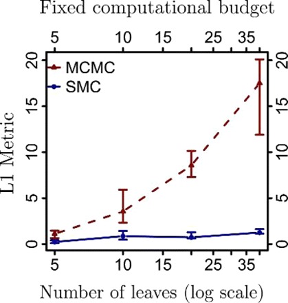
L1 distances of the minimum Bayes risk reconstruction to the true generating tree (averaged over trees and executions) as a function of the tree size (number of leaves on a log scale), measured for SMC algorithms run with 1000 particles and MCMC algorithms run for 1000 iterations.

FIGURE 5.

Analysis of the same data as in Figure 3, for 20 leaves, but with different metrics: L2 and Partition metrics, respectively.

Varying Proposals, Priors, and Likelihoods

In this section, we explore the effect of changing proposals, priors, and likelihood models. We also present results measured by wall clock times.

We first consider data generated from coalescent trees. The proposal distribution is used to choose the trees in a partial state that are merged to create a new tree (in the successor partial state) as well as the diameter of the new state. In Figure 6, we compare two types of proposal distributions, PriorPrior, described in the previous section, and PriorPost (Teh et al. 2008). PriorPost chooses the diameter of the state from the prior and then chooses the pair of trees to merge according to a multinomial distribution with parameters given by the likelihoods of the corresponding new states. (We provide further discussion of this proposal and PriorPrior in Appendix 2.) Although these proposals were investigated experimentally in Teh et al. (2008), their running times were not compared in a satisfactory manner in that work. In particular, the running time was estimated by the number of particles. This is problematic since for a given binary X-tree, PriorPost uses $O\left(\right|X{|}^3)$ peeling recurrences per particle, whereas PriorPrior uses only O(|X |) recurrences per particle. Since we measure running time by the number of peeling recurrences, our methodology does not have this problem. Surprisingly, as shown in Figure 6, PriorPrior outperforms the more complicated PriorPost by one order of magnitude. We believe that this is because PriorPost uses a larger fraction of its computational budget for the recent speciation events compared with PriorPrior, whereas the more ancient speciation events may require more particles to better approximate the uncertainty at that level. (e.g., suppose, we have a budget of $O\left(\right|X{|}^3)$ peeling recurrences. A PriorPrior sampler can use $O\left(\right|X{|}^2)$ particles and leverages $O\left(\right|X{|}^2)$ peeling recurrence for proposing the top branch lengths. A PriorPost sampler can use only O(1) particles and therefore uses only O(1) peeling recurrences for proposing the top branch lengths.)

FIGURE 6.

Comparison of two types of SMC proposal distributions.

Figure 7 shows the results for data generated by Yule processes (Rannala and Yang 1996) and uniform-branch-length trees. We see that PosetSMC is superior to MCMC in these settings as well.

FIGURE 7.

Experiments with trees generated from different models. We consider data generated by Yule processes and uniform-branch-length trees. We compare the L1 distance of the minimum Bayes reconstruction with the true generating tree for PosetSMC and MCMC.

Next, we did experiments using a different type of data: synthetic gene frequency. We used Brownian motion to generate frequencies, based the likelihood function on the same model as before and a coalescent prior. As a baseline, we used an MCMC sampler based on standard proposals (Lakner et al. 2008) (stochastic nearest neighbor interchange, global and local multiplicative branch rescaling), with four tempering chains (Neal 1996). Our implementations of continuous-character MCMC and SMC use the same code for computing the likelihood. We verified this code by comparing likelihood values against CONTML (Felsenstein 1973). Since computing the peeling dynamic program is the computational bottleneck for both SMC and MCMC, it is meaningful to compare wall clock times.

The results are shown in Figure 8. In both experiments, there is again a wide computational regime where SMC outperforms MCMC.

FIGURE 8.

Experiments on synthetic gene frequencies using a Brownian motion likelihood model. We show results for two tree sizes. In each case, we plot the partition metric as a function of the wall time in milliseconds, shown on a log scale

Experiments on Real Data

We also tested our algorithm on a comparative RNA data set (Cannone et al. 2002) containing hand-aligned ribosomal RNA. We sampled 16S components from the three domains of life at random to create multiple data sets.

We use the log likelihood of the consensus tree to evaluate the reconstructions. Since finding states of high density is necessary but not sufficient for good posterior approximation, this provides only a partial picture of how well the samplers performed. Since the true tree is not known, however, this gives a sensible surrogate.

We show the results in Figure 9. As in the synthetic data experiments, we found that the PosetSMC sampler required around two orders of magnitude less time to converge to a good approximation of the posterior. Moreover, the advantage of PosetSMC over MCMC becomes more pronounced as the number of taxa increases. For large numbers of iterations and particles, the MCMC sampler slightly outperformed the PosetSMC sampler on the real data we used.

FIGURE 9.

Results on ribosomal RNA data (Cannone et al. 2002) on different tree sizes, comparing the log likelihood of the minimum Bayes risk reconstruction from SMC and MCMC approximations, as a function of the running time (in units of the number of peeling recursions on a log scale).

We also performed experiments on frequency data from the Human Genome Diversity Panel. In these experiments, we subsampled 11,511 Single Nucleotide Polymorphisms to reduce site correlations, and we used the likelihood model based on Brownian motion described in the previous section. We show the results in Figure 10, using the log likelihood of the consensus tree as an evaluation surrogate. This shows once again the advantages of SMC methods. To give a qualitative idea of what the likelihood gains mean, we show in Figure 11 the consensus tree from 10,000 MCMC iterations versus the consensus tree from 10,000 PosetSMC particles (the circled data points). Since both runs are under sampled, the higher-order groupings are incorrect in both trees, but we can see that more mid- and low-order ethnic/geographic groupings are already captured by SMC. Incidentally, the position of the circled data points show that in practice, K SMC particles are cheaper to compute than K MCMC iterations. This is because fewer memory writes are necessary in the former case.

FIGURE 10.

Results on human gene frequency data (Li et al. 2008), comparing the log likelihood of the minimum Bayes risk reconstruction from SMC and MCMC approximations, as a function of the running time (in milliseconds, on a log scale).

FIGURE 11.

In this figure, we give a qualitative interpretation for the difference in log likelihood in Figure 10 for the consensus tree obtained from SMC with 10,000 particles and from MCMC with 10,000 iterations. Since both runs are under sampled, the higher-order groupings are incorrect in both trees, but we can see that more mid- and low-order ethnic/geographic groupings are already captured by SMC.

DISCUSSION

We have presented a general class of SMC methods that provide an alternative to MCMC for Bayesian inference in phylogeny. By making use of the order-theoretic notion of a poset, our PosetSMC methods are able to exploit the recursive structure of phylogenetic trees in computing Bayesian posteriors and marginal likelihoods. Experimental results are quite promising, showing that PosetSMC can yield significant speedups over MCMC; moreover, the relative improvement over MCMC appears to increases as the number of taxa increases, even for simple proposal distributions.

Although we have used simple likelihoods in our experiments, it is also possible to incorporate state-of-the-art models in our framework. Whenever the likelihood for a given tree can be computed exactly and efficiently in a bottom-up manner, our framework applies directly. This includes, for example, models based on more sophisticated rate matrices such as the generalized time-reversible model (Tavaré 1986), covarion models (Penny et al. 2001), approximate context-dependent models (Siepel and Haussler 2004), and fixed-alignment insertion-deletion-aware models (Rivas 2005).

It is also possible to accommodate models that require alternating sampling of parameters and topology, such as random rate matrix and relaxed-clock models (Thorne et al. 1998, Huelsenbeck et al. 2000, Drummond et al. 2006) and insertion–deletion models with alignment resampling (Redelings and Suchard 2005). This can be done by making use of the Particle Markov chain Monte Carlo (PMCMC) method introduced in Andrieu et al. (2010). PMCMC is a hybrid of MCMC and SMC in which an SMC algorithm is used as a proposal in an MCMC chain. Remarkably, it is possible to compute the acceptance ratio for this complex proposal exactly, directly from the output of SMC algorithm. Each factor in the acceptance ratio is computed from the data likelihood estimator of Equation (3): If we denote the estimate of Equation (3) for the current and previous MCMC iteration by L^′ and L, respectively, then the acceptance ratio is simply $\text{min}\{1,L^{\prime }/L\}$.

As alluded to earlier, an important advantage of SMC over MCMC is the ease in which it can adapt to parallel architectures. Indeed, the peeling recurrence when computing the proposals is the bottleneck in PosetSMC, and this computation can be easily parallelized by distributing particles across cores. Distribution across clusters is also possible. Note that by exchanging particles across machines after computing the resampling step, it is possible to avoid moving around many particles. In contrast, parallelization of MCMC phylogenetic samplers is possible (Feng et al. 2003, Altekar et al. 2004, Keane et al. 2005, Suchard and Rambaut 2009) but is not as direct. Moreover, all three main approaches to MCMC parallelization have limitations: The first method is to parallelize the likelihood computation, including Graphics Processing Unit parallelization; when scale comes from a large number of taxa, however, this approach reaches its limits. The second method involves running several independent chains; however, this approach suffers from a lack of communication across processors: If one processor finds a way of getting out of a local optimum, it has no way of sharing this information with the other nodes. The third method is to augment the MCMC chain using auxiliary variables, for example, by using parallel tempering (Swendsen and Wang 1986), or multiple-try Metropolis–Hastings (Liu et al. 2000). However, these state augmentations induce trade-offs between computational efficiency and statistical efficiency.

A practical question in the application of PosetSMC is the choice of K, the number of particles. Although this choice depends on the specific test functions that are being estimated, one generic measure of the accuracy of the PosetSMC estimator can be based on the effective sample size (ESS) (Kong et al. 1994)—the number of independent samples from the true posterior required to obtain an estimator with the same variance as the PosetSMC estimator. A small ESS (relative to K) is indicative that the SMC is inefficient. Such inefficiencies might be alleviated by increasing K or by changing the proposals. One method for estimating ESS in the context of classical SMC (Carpenter et al. 1999) can be applied here. The idea is to run PosetSMC on the same data L times for a fixed K. For scalar functions ϕ, the ratio of the variance of ϕ estimated within each run to the variance estimated across the L runs is an estimate of ESS.

PosetSMC algorithms can also benefit from improved sampling techniques that have been developed for other SMC algorithms. For example, standard techniques such as stratified sampling (Kitagawa 1996) or adaptive resampling (Moral et al. 2011) can be readily applied. Other potential improvements are reviewed in Cappé et al. (2005) and Doucet and Johansen (2009).

Note finally that the poset framework applies beyond phylogenetic tree reconstruction. Other examples of Bayesian inference problems in computational biology that may benefit from the PosetSMC framework include statistical alignment for proteins and DNA and grammatical inference for RNA.

FUNDING

This work was supported by the National Institutes of Health [R01 GM071749]; and the Department of Energy [SciDAC BER KP110201].

APPENDIX 1

Proof of Consistency

In this section, we prove Proposition 4. The proof is similar conceptually to proofs of consistency for non-poset frameworks (Crisan and Doucet 2002, Moral 2004, Douc and Moulines 2008), with the main points of interest being the specific ways in which Assumptions 1, 2, and 3 are invoked to permit the generalization to posets. For simplicity, we present the argument for convergence in $L^2$ here (using → to denote convergence in $L^2$), assuming bounded ${\gamma }_{*}$; see Moral (2004) for many extensions, including strong laws and central limit theorems.

Proof. We start by introducing a measure ${\lambda }_{r,K}$ for the unnormalized distribution over the particles proposed at an SMC iteration r with K particles. From Assumption 1 and 2(b), we see that λ has the following form, for r >0 and all $A\in {ℱ}_{𝒮}$:

Note that in this section, we view ${\pi }_{r,k}$ and hence ${\lambda }_{r,K}$ as random variables, so we will need a notation for the limit as K →∞ of the ${\lambda }_{r,K}$ measures, which, as we will see shortly, has the form:

where ${\pi }_r$ is defined with the following Radon–Nikodym derivative relative to a dominating base measure μ:

The main step of the proof is to show by induction on r that:

(7)

(8)

for any integrable ${\varphi }_{*}:𝒮\to ℝ$, at a rate of C/n. This is sufficient since Equation (4) can be obtained by taking the product over Equation (7) for r ∈{1,⋯,R}, and Equation (5), by specializing Equation (8) to r = R with ${\varphi }_{*}\left(s\right)=\varphi \left(s\right)$ for s ∈ 𝒯 and ${\varphi }_{*}\left(s\right)=0$ otherwise, and by using Assumption 3(b).

The base case is a standard importance sampling argument, so we concentrate on the induction step.

Note first that by Assumptions 1 and 2(a, b), the weight $w_{r,k}$ is a deterministic function of $s_{r,k}$: Since the poset is acyclic and connected, there exists a unique $s_{r-1,k}$ covered by $s_{r,k}$, denoted by $\left(s_{r,k}\right)$ which gives all the ingredients needed to compute Equation (2). Moreover, by the Radon–Nikodym theorem and Assumptions 1, 2(a), and 3(a), this function can be written as the product of two derivatives as follows:

We will let the number of particles at generation r and $r^{\prime }<r$ go to infinity separately, using the notation ${\pi }_{r,K^{\prime },K_r}$.

By applying the law of large numbers, we obtain (using the fact that the weights are bounded and uncorrelated):

Next, by applying the induction hypothesis to Equation (8) with r − 1 and $\varphi ={\nu }_{·}$, we get that

Therefore, by setting $K=K^{\prime }=K_r$, we get:

using $\parallel {\lambda }_r\parallel =\parallel {\pi }_{r-1}\parallel$ since the proposals ν_· are assumed to be normalized. There is also a limit interchange argument for this step that can be formalized using the rates of convergence and the Minkowski inequality.

To prove the other induction component, Equation (8), we first use Equation (7) to rewrite the weight normalization and then proceed similarly to the above argument:

          □

APPENDIX 2

Weight Updates

In this section, we simplify Equation (2) in the case of PriorPrior and PriorPost proposals on coalescent trees, showing that the updates of Teh et al. (2008) are recovered in these special cases.

In both cases, given a partial state s, a successor partial state (forest), $s^{\prime }$, is obtained from a previous partial state s by merging two trees, $t_l$ and $t_r$, creating a new tree $t_m$ (see Fig. A1). Formally, we have that $q(s\to s^{\prime })>0$ implies that there are disjoint sets $X_l=X_l(s^{\prime }),X_r=X_r(s^{\prime })$ such that:

FIGURE A1.

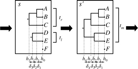
A partial state s is extended to a new partial partial state $s^{\prime }$ by merging trees $t_l$ and $t_r$ to form a tree $t_m$ with height $h_4>h_3$. In the PriorPrior proposal, $t_l$ and $t_r$ are chosen uniformly from the three possible pairs, whereas the height increment ${\delta }_4$ is chosen from an exponential distribution. In the PriorPost proposal, ${\delta }_4$ is chosen from the exponential prior and, given ${\delta }_4$, the pair to merge is chosen from a multinomial with parameters proportional to the likelihood of the tree $t_m$.

where $X_m=X_m(s^{\prime })=X_l\cup X_r$, and $t_m=t_m\left(s^{\prime }\right)$ is an $X_m$-tree in which both $t_l=t_l\left(s^{\prime }\right)$ and $t_r=t_r\left(s^{\prime }\right)$ occur as subtrees. As mentioned in the main text, the new forest is also required to be strictly taller. To formalize this, consider an ordering of the speciation events in a forest s, where the heights of these events are indexed in the order they were created in the path of partial states leading to s, $0=h_0,h_1,\cdots ,h_{\rho \left(s\right)}$. Letting ${\delta }_i\left(s\right)=h_i-h_{i-1}$ denote the height increments, we require that for all i, ${\delta }_i\left(s\right)>0$ with probability one. We denote the tree $t_m$ by $m_s(t_l,t_r,\delta )$, where $\delta =\delta (s^{\prime })={\delta }_{\rho (s^{\prime })}\left(s^{\prime }\right)$. The set of possible successor trees is denoted by S(s), and the subset of successors with top increment δ is denoted by $S_{\delta }\left(s\right)=\{s^{\prime }\in S\left(s\right):\delta (s^{\prime })=\delta \}$.

PriorPrior and PriorPost also share the same extension, ${\gamma }_{*}$, which is a product of three factors: one for the topology prior, one for the branch length prior, and one for the likelihood model $L_{𝒴}\left(t\right)$. The first prior factor is uniform over forest topologies, and so, this first factor can be ignored since ${\gamma }_{*}$ is only needed up to a normalization constant. The second prior factor is written as a distribution over height increments, where ${\Delta }_i\left(\delta \right)$ is an exponential density for the coalescent prior: Finally, multiplying the likelihood by the prior yields:

where we use the symbol ∝ to mean that the expression is defined up to a proportionality constant that can only depend on s via |s|.

We now consider the cancellations possible in Equation (2) when the PriorPrior proposal,

is used:

Note that cancellations such as these are not necessary to implementing PosetSMC; indeed, they do not play a significant computational role. Our goal in presenting them was simply to make precise the connection with Teh et al. (2008).

In the PriorPost proposal, a height increment is first sampled from ${\Delta }_{\rho (s^{\prime })}$, then, conditioning on this increment δ, the likelihood ratios

are computed for all $s^{\prime }\in S_{\delta }\left(s\right)$. These ratios are then normalized and become the parameters of a multinomial proposal over the pair of trees to coalesce:

We get the following simplified form of Equation (2) for PriorPost:

Finally, we show how these weight updates can alternatively (but less transparently) be expressed as the normalization of a specific version of the peeling recursion. Let ${𝒴}_j$ denote observations for site j and let ${\xi }_{j,t}$ denote the internal (hidden) nucleotide random variable at site j at the root of t. The recursion in question is:

where Therefore, the weight updates can be obtained as functions of the product of the normalizations of the top-level recursions.

REFERENCES

- Altekar G, Dwarkadas S, Huelsenbeck JP, Ronquist F. Parallel Metropolis coupled Markov chain Monte carlo for Bayesian phylogenetic inference. Bioinformatics. 2004;20:407–415. doi: 10.1093/bioinformatics/btg427. [DOI] [PubMed] [Google Scholar]
- Andrieu C, Doucet A, Holenstein R. Particle Markov chain Monte Carlo methods. J. R. Stat. Soc. Series B. Stat. Methodol. 2010;72:269–342. [Google Scholar]
- Beaumont MA, Zhang W, Balding DJ. Approximate Bayesian computation in population genetics. Genetics. 2002;162:2025–2035. doi: 10.1093/genetics/162.4.2025. [DOI] [PMC free article] [PubMed] [Google Scholar]
- Bourque M. Arbres de Steiner et réseaux dont certains sommets sont à localisation variable [PhD dissertation]. Montreal (QC): Université de Montréal. 1978 [Google Scholar]
- Cannone JJ, Subramanian S, Schnare MN, Collett JR, D'Souza LM, Du Y, Feng B, Lin N, Madabusi LV, Muller KM, Pande N, Shang Z, Yu N, Gutell RR. The comparative RNA web (CRW) site: an online database of comparative sequence and structure information for ribosomal, intron, and other RNAs. BMC Bioinformatics. 2002;3:2. doi: 10.1186/1471-2105-3-2. [DOI] [PMC free article] [PubMed] [Google Scholar]
- Cappé O, Moulines E, Rydén T. Inference in hidden Markov models. New York: Springer; 2005. [Google Scholar]
- Carpenter J, Clifford P, Fearnhead P. An improved particle filter for non-linear problems. IEE Proceedings: Radar. Sonar and Navigation. 1999;Volume 146:2–7. [Google Scholar]
- Crisan D, Doucet A. A survey of convergence results on particle filtering for practitioners. IEEE Trans. Signal Process. 2002;50:736–746. [Google Scholar]
- Doob JL. Markoff chains—denumerable case. Trans. Amer. Math. Soc. 1945;58:455–473. [Google Scholar]
- Douc R, Moulines E. Limit theorems for weighted samples with applications to sequential Monte Carlo methods. Ann. Stat. 2008;36:2344–2376. [Google Scholar]
- Doucet A, Freitas ND, Gordon N. Sequential Monte Carlo methods in practice. New York: Springer; 2001. [Google Scholar]
- Doucet A, Johansen AM. Cambridge (UK): Cambridge University Press; 2009. A tutorial on particle filtering and smoothing: fifteen years later. [Google Scholar]
- Drummond AJ, Ho SYW, Phillips MJ, Rambaut A. Relaxed phylogenetics and dating with confidence. PLoS Biol. 2006 doi: 10.1371/journal.pbio.0040088. 4:e88. [DOI] [PMC free article] [PubMed] [Google Scholar]
- Fan Y, Wu R, Chen M-H, Kuo L, Lewis PO. Choosing among partition models in Bayesian phylogenetics. Mol. Biol. Evol. 2011;28:523–532. doi: 10.1093/molbev/msq224. [DOI] [PMC free article] [PubMed] [Google Scholar]
- Felsenstein J. Maximum-likelihood estimation of evolutionary trees from continuous characters. Am. J. Hum. Genet. 1973;25:471–492. [PMC free article] [PubMed] [Google Scholar]
- Felsenstein J. Evolutionary trees from DNA sequences: a maximum likelihood approach. J. Mol. Evol. 1981;17:368–376. doi: 10.1007/BF01734359. [DOI] [PubMed] [Google Scholar]
- Felsenstein J. Sunderland (MA): Sinauer Associates; 2003. Inferring phylogenies. [Google Scholar]
- Feng X, Buell DA, Rose JR, Waddell PJ. Parallel algorithms for Bayesian phylogenetic inference. J. Parallel. Distrib. Comput. 2003;63:707–718. [Google Scholar]
- Gelman A, Meng X-L. Simulating normalizing constants: from importance sampling to bridge sampling to path sampling. Stat. Sci. 1998;13:163–185. [Google Scholar]
- Görür D, Teh YW. Advances in neural information processing. Red Hook (NY): Curran Associates; 2008. An efficient sequential Monte-Carlo algorithm for coalescent clustering; pp. 521–528. [Google Scholar]
- Griffiths RC, Tavaré S. Monte Carlo inference methods in population genetics. Math. Comput. Model. 1996;23:141–158. [Google Scholar]
- Huelsenbeck JP, Larget B, Swofford D. A compound Poisson process for relaxing the molecular clock. Genetics. 2000;154:1879–1892. doi: 10.1093/genetics/154.4.1879. [DOI] [PMC free article] [PubMed] [Google Scholar]
- Huelsenbeck JP, Ronquist F. MRBAYES: Bayesian inference of phylogenetic trees. Bioinformatics. 2001;17:754–755. doi: 10.1093/bioinformatics/17.8.754. [DOI] [PubMed] [Google Scholar]
- Huelsenbeck JP, Ronquist F, Nielsen R, Bollback JP. Bayesian inference of phylogeny and its impact on evolutionary biology. Science. 2001;294:2310–2314. doi: 10.1126/science.1065889. [DOI] [PubMed] [Google Scholar]
- Iorio MD, Griffiths RC. Importance sampling on coalescent histories. Adv. Appl. Probab. 2004;36:417–433. [Google Scholar]
- Keane TM, Naughton TJ, Travers SAA, McInerney JO, McCormack GP. DPRml: distributed phylogeny reconstruction by maximum likelihood. Bioinformatics. 2005;21:969–974. doi: 10.1093/bioinformatics/bti100. [DOI] [PubMed] [Google Scholar]
- Kimura M. A simple method for estimating evolutionary rate of base substitutions through comparative studies of nucleotide sequences. J. Mol. Evol. 1980;16:111–120. doi: 10.1007/BF01731581. [DOI] [PubMed] [Google Scholar]
- Kitagawa G. Monte Carlo filter and smoother for non-Gaussian nonlinear state space models. J. Comput. Graph. Stat. 1996;5:1–25. [Google Scholar]
- Kong A, Liu JS, Wong WH. Sequential imputations and Bayesian missing data problems. J. Am. Stat. Assoc. 1994;89:278–288. [Google Scholar]
- Kuhner MK, Felsenstein J. A simulation comparison of phylogeny algorithms under equal and unequal evolutionary rates. Mol. Biol. Evol. 1994;11:459–468. doi: 10.1093/oxfordjournals.molbev.a040126. [DOI] [PubMed] [Google Scholar]
- Lakner C, der Mark PV, Huelsenbeck JP, Larget B, Ronquist F. Efficiency of MCMC proposals in Bayesian phylogenetics. Syst. Biol. 2008;57:86–103. doi: 10.1080/10635150801886156. [DOI] [PubMed] [Google Scholar]
- Lartillot N, Philippe H. Computing Bayes factors using thermodynamic integration. Syst. Biol. 2006;55:195–207. doi: 10.1080/10635150500433722. [DOI] [PubMed] [Google Scholar]
- Li JZ, Absher DM, Tang H, Southwick AM, Casto AM, Ramachandran S, Cann HM, Barsh GS, Feldman M, Cavalli-Sforza LL, Myers RM. Worldwide human relationships inferred from genome-wide patterns of variation. Science. 2008;319:1100–1104. doi: 10.1126/science.1153717. [DOI] [PubMed] [Google Scholar]
- Liu JS, Liang F, Wong WH. The multiple-try method and local optimization in Metropolis sampling. J. Am. Stat. Assoc. 2000;95:121–134. [Google Scholar]
- Marjoram P, Molitor J, Plagnol V, Tavaré S. Markov chain Monte Carlo without likelihoods. Proc. Natl. Acad. Sci. U.S.A. 2002;100:15324–15328. doi: 10.1073/pnas.0306899100. [DOI] [PMC free article] [PubMed] [Google Scholar]
- Moral PD. Feynman-Kac formulae. New York: Springer; 2004. [Google Scholar]
- Moral PD, Doucet A, Jasra A. Sequential Monte Carlo samplers. J. R. Stat. Soc. Series B. Stat. Methodol. 2006;68:411–436. [Google Scholar]
- Moral PD, Doucet A, Jasra A. On adaptive resampling strategies for sequential Monte Carlo methods. Bernoulli. 2012;12:252–278. [Google Scholar]
- Neal RM. Sampling from multimodal distributions using tempered transitions. Stat. Comput. 1996;6:353–366. [Google Scholar]
- Newton MA, Raftery AE. Approximate Bayesian inference with the weighted likelihood bootstrap. J. R. Stat. Soc. Series B. Stat. Methodol. 1994;56:3–48. [Google Scholar]
- Paul JS, Steinrücken M, Song YS. An accurate sequentially Markov conditional sampling distribution for the coalescent with recombination. Genetics. 2011;187:1115–1128. doi: 10.1534/genetics.110.125534. [DOI] [PMC free article] [PubMed] [Google Scholar]
- Penny D, McComish BJ, Charleston MA, Hendy MD. Mathematical elegance with biochemical realism: the covarion model of molecular evolution. J. Mol. Evol. 2001;53:711–723. doi: 10.1007/s002390010258. [DOI] [PubMed] [Google Scholar]
- Rannala B, Yang Z. Probability distribution of molecular evolutionary trees: a new method of phylogenetic inference. J. Mol. Evol. 1996;43:304–311. doi: 10.1007/BF02338839. [DOI] [PubMed] [Google Scholar]
- Redelings B, Suchard M. Joint Bayesian estimation of alignment and phylogeny. Syst. Biol. 2005;54:401–418. doi: 10.1080/10635150590947041. [DOI] [PubMed] [Google Scholar]
- Rivas E. Evolutionary models for insertions and deletions in a probabilistic modeling framework. BMC Bioinformatics. 2005;6:63. doi: 10.1186/1471-2105-6-63. [DOI] [PMC free article] [PubMed] [Google Scholar]
- Robert CP. The Bayesian choice: from decision-theoretic foundations to computational implementation. New York: Springer; 2001. [Google Scholar]
- Robinson DF, Foulds LR. Comparison of phylogenetic trees. Math. Biosci. 1981;33:131–147. [Google Scholar]
- Saitou N, Nei M. The neighbor-joining method: a new method for reconstructing phylogenetic trees. Mol. Biol. Evol. 1987;4:406–425. doi: 10.1093/oxfordjournals.molbev.a040454. [DOI] [PubMed] [Google Scholar]
- Semple C, Steel M. Phylogenetics. Oxford: Oxford University Press; 2003. [Google Scholar]
- Siepel A, Haussler D. Phylogenetic estimation of context-dependent substitution rates by maximum likelihood. Mol. Biol. Evol. 2004;21:468–488. doi: 10.1093/molbev/msh039. [DOI] [PubMed] [Google Scholar]
- Suchard MA, Rambaut A. Many-core algorithms for statistical phylogenetics. Bioinformatics. 2009;25:1370–1376. doi: 10.1093/bioinformatics/btp244. [DOI] [PMC free article] [PubMed] [Google Scholar]
- Swendsen RH, Wang JS. Replica Monte Carlo simulation of spin glasses. Phys. Rev. Lett. 1986;57:2607–2609. doi: 10.1103/PhysRevLett.57.2607. [DOI] [PubMed] [Google Scholar]
- Tavaré S. Some probabilistic and statistical problems in the analysis of DNA sequences. Lect. Math. Life Sci. 1986;17:57–86. [Google Scholar]
- Teh YW, Daume H, 3rd, Roy DM. Cambridge (MA): MIT Press; 2008. Bayesian agglomerative clustering with coalescents. Advances in neural information processing; pp. 1473–1480. [Google Scholar]
- Thorne JL, Kishino H, Painter IS. Estimating the rate of evolution of the rate of molecular evolution. Mol. Biol. Evol. 1998;15:1647–1657. doi: 10.1093/oxfordjournals.molbev.a025892. [DOI] [PubMed] [Google Scholar]
- Tom JA, Sinsheimer JS, Suchard MA. Reuse, recycle, reweigh: combating influenza through efficient sequential Bayesian computation for massive data. Ann. Appl. Stat. 2010;4:1722–1748. doi: 10.1214/10-AOAS349. [DOI] [PMC free article] [PubMed] [Google Scholar]
- Xie W, Lewis PO, Fan Y, Kuo L, Chen M-H. Improving marginal likelihood estimation for Bayesian phylogenetic model selection. Syst. Biol. 2011;60:150–160. doi: 10.1093/sysbio/syq085. [DOI] [PMC free article] [PubMed] [Google Scholar]