A General Framework for Two-Stage Analysis of Genome-wide Association Studies and Its Application to Case-Control Studies

Abstract

Two-stage analyses of genome-wide association studies have been proposed as a means to improving power for designs including family-based association and gene-environment interaction testing. In these analyses, all markers are first screened via a statistic that may not be robust to an underlying assumption, and the markers thus selected are then analyzed in a second stage with a test that is independent from the first stage and is robust to the assumption in question. We give a general formulation of two-stage designs and show how one can use this formulation both to derive existing methods and to improve upon them, opening up a range of possible further applications. We show how using simple regression models in conjunction with external data such as average trait values can improve the power of genome-wide association studies. We focus on case-control studies and show how it is possible to use allele frequencies derived from an external reference to derive a powerful two-stage analysis. An illustration involving the Wellcome Trust Case-Control Consortium data shows several genome-wide-significant associations, subsequently validated, that were not significant in the standard analysis. We give some analytic properties of the methods and discuss some underlying principles.

Introduction

Although there is consensus on simple methods of primary statistical analysis in genome-wide association studies (GWASs), there have been continuing efforts to develop more powerful approaches as the vast extent of polygenic heritability of complex traits has become apparent.^1,2 A strategy that has received much attention is that of reducing the inherent multiplicity by performing a two-stage analysis. In the first stage, a preliminary screening of markers is performed, and this is followed by a final analysis on a subset of markers with a reduced multiple-testing adjustment. For example, it can be cost efficient to perform the full GWAS on a subset of the study sample but to hold back the remainder for a confirmatory analysis of the most promising markers.^3,4 Alternatively, one can analyze all data in different ways at each stage and use each analysis to reduce the number of tests performed.^5,6

In this paper we are concerned with a class of two-stage approaches in which a single sample is analyzed twice with two independent statistics. In the first pass, the data are analyzed with a statistic that is valid only under some underlying assumptions. The markers that are selected from this stage are then analyzed in a second pass via an independent test that is robust to the assumptions in question. Because the statistics in the two stages are independent by construction, the final multiplicity depends only on the markers tested in the second stage; these markers are potentially much fewer than those in the first stage.

This approach was initiated in the context of family-based association tests of quantitative traits.⁷ The standard analysis is a within-family test that is robust to population stratification, but a first-stage analysis can be performed with between-family information that might be confounded by stratification. Reasonable gains in power over standard GWAS analysis have been postulated,⁸ and the method has been adapted for binary traits.⁹

A related approach has been developed for tests of gene-environment interaction.¹⁰ The traditional test compares the gene-environment association in cases to the same quantity in controls. In the two-stage approach, the first stage tests the marginal gene-environment association in a full case-control sample. This test is independent of the traditional test but assumes that the gene and environment are not associated in the source population. Again, simulations have demonstrated that using this approach results in potential gains in power.

An approach for gene-gene interaction uses the two marginal gene-disease associations in the first stage.¹¹ Although this is also a two-stage method, it is somewhat different from the methods discussed here because the two stages are not independent (although in practice they are nearly so) and because there is no additional assumption needed in stage 1. Recent work has adapted this idea to gene-environment interaction and has shown that it can offer small improvements over the earlier method.¹²

Another two-stage approach has been proposed for case-control analysis. In this approach, the first stage compares the deviation from Hardy-Weinberg equilibrium (HWE) in cases to that in controls.¹³ The second stage uses a standard test of the trend in log-odds of disease. This approach is of limited use in real GWASs because most associations found to date have followed a log-additive model of risk, under which both cases and controls would follow HWE and the first stage would have no power.

In this paper we propose a general formulation of two-stage approaches in terms of constructing two independent estimators of a single quantity. We show how family-based and gene-environment strategies can be expressed in this formulation and show how the principle can be generalized to a wide range of analyses. We focus on linear models and show that when external reference information, such as allele frequencies or trait means, is available, it can serve to improve the power of a GWAS while retaining robustness to mis-specification of that information. Illustrating our approach on data from the Wellcome Trust Case-Control Consortium (WTCCC),¹⁴ we identify as significant several regions that were not significant in the original analysis but whose association with disease has been validated by follow-up studies.

Material and Methods

Construction of Two-Stage Analysis

We consider the analysis of individual markers within a GWAS. For ease of exposition, we assume the markers are diallelic and have additive effects on an appropriate scale, but our analysis and results generalize without difficulty. Suppose we are concerned with the effect of a marker expressed by a parameter ${\beta }_1$. A motivating example is the linear regression model in which the trait Y of a subject is related to its genotype by $E\left(Y|X\right)={\beta }_0+{\beta }_{1}X$, where x denotes the number of minor alleles carried. Then the usual null hypothesis is H₀:β₁ = 0, which may be tested by a Wald test on the maximum likelihood estimator (MLE) ${\hat{\beta }}_1$. This will form the basis of the second stage of the analysis.

Suppose that the trait also depends on a nuisance parameter β₀, which we will also estimate from the data. In the linear regression example, β₀ is the intercept. Now let us postulate a fixed value ${\beta }_0^{\ast }$ a priori. If indeed ${\beta }_0={\beta }_0^{\ast }$, then ${\beta }_1={\beta }_1+s\left({\beta }_0-{\beta }_0^{\ast }\right)$ for any s. Notice that (1) ${\hat{\beta }}_1+s\left({\hat{\beta }}_0-{\beta }_0^{\ast }\right)$ and ${\hat{\beta }}_1$ can be written as A + B and A − B, where $A={\hat{\beta }}_1+\frac{1}{2}s\left({\hat{\beta }}_0-{\beta }_0^{\ast }\right)$ and $B=\frac{1}{2}s\left({\hat{\beta }}_0-{\beta }_0^{\ast }\right)$ and that (2) if ${\hat{\beta }}_0$ and ${\hat{\beta }}_1$ are MLEs, then A and B are asymptotically normally distributed. If A and B have the same variance and are normally distributed, then A + B and A − B are independent. Thus by choosing s such that $\mathrm{var}\left({\hat{\beta }}_1+\frac{1}{2}s\left({\hat{\beta }}_0-{\beta }_0^{\ast }\right)\right)=\mathrm{var}\left(\frac{1}{2}s\left({\hat{\beta }}_0-{\beta }_0^{\ast }\right)\right)$, we can form an estimator for ${\beta }_1$ that is asymptotically independent of ${\hat{\beta }}_1$. A calculation gives $s=-\mathrm{var}\left({\hat{\beta }}_1\right)/\mathrm{cov}\left({\hat{\beta }}_0,{\hat{\beta }}_1\right)$.

We therefore have the following general two-stage procedure:

Stage 1: calculate ${\hat{\beta }}_1+s\left({\hat{\beta }}_0-{\beta }_0^{\ast }\right)$ for all markers, where $s=-\mathrm{var}\left({\hat{\beta }}_1\right)/\mathrm{cov}\left({\hat{\beta }}_0,{\hat{\beta }}_1\right)$, and let $T_1={\hat{\beta }}_1+s\left({\hat{\beta }}_0-{\beta }_0^{\ast }\right)/SE\left({\hat{\beta }}_1+s\left({\hat{\beta }}_0-{\beta }_0^{\ast }\right)\right)$.

Stage 2: for all markers for which $\left|T_1\right|>t_1$, where t₁ is a fixed threshold, calculate $T_2={\hat{\beta }}_1/SE\left({\hat{\beta }}_1\right)$. Declare as significant those markers for which $\left|T_2\right|>t_2$, where t₂ is chosen such that under H₀, $\mathrm{Pr}\left(\left|T_2\right|>t_2\right)=M\alpha /m_0$, where α is the target type 1 error rate per marker, M is the total number of markers, and m₀ is the number of markers carried forward from stage 1.

The first-stage threshold t₁ should be high enough to eliminate many null markers from stage 2 but low enough to permit most associated markers to pass stage 1. We discuss the choice of t₁ later. The two key properties of this procedure are as follows: (1) if the postulated value ${\beta }_0^{\ast }$ is correct, then ${\hat{\beta }}_1+s\left({\hat{\beta }}_0-{\beta }_0^{\ast }\right)$ and ${\hat{\beta }}_1$ are two independent estimators of the same quantity ${\beta }_1$; and (2) whether or not ${\beta }_0^{\ast }$ is correct, the two estimators remain independent, and the two-stage procedure maintains the specified type 1 error rate.¹⁰ We note that score or likelihood-ratio tests could be used in place of T₁ and T₂ because of their asymptotic equivalence to the Wald tests. The Wald tests are needed for the formal definition of the procedure because they are independent by construction.

In some circumstances we might be more interested in the difference between two parameters, ${\beta }_1-{\beta }_0$, in which a postulated value ${\beta }_0^{\ast }$ is again available. An example of such a difference might be that in allele frequencies between cases and controls. By similar arguments, we then base stage 1 on

$${\hat{\beta }}_1-{\hat{\beta }}_0+s\left({\hat{\beta }}_0-{\beta }_0^{\ast }\right),$$

where

$$s=\frac{\mathrm{var}\left({\hat{\beta }}_1\right)+\mathrm{var}\left({\hat{\beta }}_0\right)-2\mathrm{cov}\left({\hat{\beta }}_0,{\hat{\beta }}_1\right)}{\mathrm{var}\left({\hat{\beta }}_0\right)-\mathrm{cov}\left({\hat{\beta }}_0,{\hat{\beta }}_1\right)}$$ (1)

and stage 2 on ${\hat{\beta }}_1-{\hat{\beta }}_0$.

The variances and covariances used in the calculation of s typically depend on the true parameters ${\beta }_0,{\beta }_1$ which are unknown. One can estimate them from the data by assuming either the null or alternative hypothesis. In common with many standard procedures, we assume the null hypothesis when estimating s, which also has the effect of reducing or removing any correlation induced between T₁ and T₂ by the estimation of standard errors.

We now show how previous two-stage methods can be expressed in this formulation, and we will then describe some additional applications.

Family-Based Association

Two-stage approaches of this type were initiated by Van Steen et al.,⁷ who considered parent-child trios in which markers are tested for association to a quantitative trait in the children. The second stage uses the FBAT test,¹⁵ whereas the first stage is based on a “conditional mean model,” which predicts the expected trait in the child given the parental genotypes. Up to technical details this approach is equivalent to one based on the orthogonal linear model of Abecasis et al.¹⁶

$$E\left(Y|X,X_M,X_F\right)=\mu +{\beta }_{b}B+{\beta }_{w}W,$$

where B = (X_M + X_F)/2, in which X_M and X_F are the number of minor alleles in the mother and father, respectively, and W = X − B. The within-family association parameter ${\beta }_w$ is unbiased for the additive effect of the minor allele, even under population stratification, whereas the between-family parameter ${\beta }_b$ is confounded by stratification. This model can be rewritten as

$$E\left(Y|X,X_M,X_F\right)=\mu +\left({\beta }_b-{\beta }_w\right)B+{\beta }_{w}X,$$

from which we see that our two-stage approach uses ${\beta }_1={\beta }_w$, ${\beta }_0={\beta }_b-{\beta }_w$ and a postulated value (under no population stratification) of ${\beta }_0^{\ast }=0$. Because ${\beta }_b$ and ${\beta }_w$ are independent by construction, we have s = 1 so that stage 1 is based on ${\beta }_b$.

For binary traits, a common design uses case-parent trios, in which case the above model cannot be used because there is no variation in Y. Murphy et al.⁹ propose an approach that is equivalent to one based on the retrospective full likelihood of Dudbridge¹⁷

$$\mathrm{Pr}\left(C|M,F,Y=1\right)=\frac{{\beta }_{w}X\left(C\right)}{\sum _{c\in S\left(M,F\right)}{\beta }_{w}X\left(c\right)}·\frac{{\alpha }_{M,F}\sum _{c\in S\left(M,F\right)}{\beta }_{b}X\left(c\right)}{\sum _{m,f}{\alpha }_{m,f}\sum _{c\in S\left(m,f\right)}{\beta }_{b}X\left(c\right)},$$ (2)

where C, M, and F are the genotypes of the child, mother, and father, respectively, X(C) is the number of minor alleles in genotype C, S(M,F) is the set of phased genotypes of the possible children of parents M and F, and ${\alpha }_{M,F}$ are additional parameters that model the mating-type frequencies. In this model, ${\hat{\beta }}_w$ and ${\hat{\beta }}_b$ are independent, and we can again apply our two-stage approach by using ${\beta }_1={\beta }_w$, ${\beta }_0={\beta }_b-{\beta }_w$, and ${\beta }_0^{\ast }=0$, which is true under no population stratification.

Murphy et al. prefer to estimate ${\beta }_b$ from certain restricted comparisons of mating-type frequencies and to thus avoid the need to estimate parameters α, which might be difficult to estimate under latent population stratification. However, their approach depends on an assumption of HWE in the population, and such an assumption is itself sensitive to population stratification. They give four estimators of ${\beta }_b$, but the optimal combination of these estimators depends on the mating-type frequencies. The advantages of using estimators of ${\beta }_b$ that are independent of α therefore seem limited.

Furthermore, under the commonly assumed multiplicative model of risk, the relative risk is identified in only one of the estimators proposed by Murphy et al. (This estimator is $R_2$ in their Equation 6). We would therefore expect their approach to be less powerful than one based on estimating ${\beta }_b$ from the full data by using the likelihood (Equation 2). We give a numerical example in the Results. The lack of a distributional theory for the estimator based on $R_2$, and the fact that this estimator is the solution of a quadratic equation that might not have real roots, also argue against the use of $R_2$ to estimate ${\beta }_b$. The between-family effect ${\beta }_b$ is estimated from (Equation 2) by the UNPHASED software,¹⁷ and we can then obtain a test of ${\hat{\beta }}_b=0$ by comparing the likelihoods of the alternative hypothesis with and without its “-parentrisk” option.

Both quantitative- and binary-trait models can be generalized to families with multiple siblings and missing parents, but this is not our focus here. The binary-trait model can be adapted for two-stage analysis of matched case-control studies because the case-parent trio design is equivalent to a matched analysis of the case and three pseudo-controls.¹⁸ The details would be straightforward and are deferred to a future study.

Gene-Environment Interaction

In the method proposed by Murcray et al., a binary environmental exposure is considered, and we wish to test whether it modifies the odds ratio of a genetic marker in a case-control study.¹⁰ The first stage treats the environment as the response and tests for a marginal association between gene and environment in the entire sample of cases and controls:

$$E\left[\text{logit}\left(\mathrm{Pr}\left(E=1|X\right)\right)\right]={\gamma }_0+{\gamma }_{g}X$$ (3)

The second stage tests the interaction term in a standard logistic regression model for case-control data

$$E\left[\text{logit}\left(\mathrm{Pr}\left(Y=1|X,E\right)\right)\right]=\mu +{\beta }_{g}X+{\beta }_{e}E+{\beta }_{ge}XE$$

To relate this method to our formulation, we note that the interaction term ${\beta }_{ge}$ is the same as that in the model with environment as outcome

$$E\left[\text{logit}\left(\mathrm{Pr}\left(E=1|X,Y\right)\right)\right]={\mu }^{\prime }+{\beta }_g^{\prime }X+{\beta }_{y}Y+{\beta }_{ge}XY,$$ (4)

so we can base the second stage on Equation 4 by setting ${\beta }_1={\beta }_{ge}$. Under the stage 1 assumption of gene-environment independence in the population, and under the assumption of a rare disease, there is no association between the gene and environment in the controls, so that ${\beta }_g^{\prime }=0$. Therefore, we can use ${\beta }_0={\beta }_g^{\prime }$ with the postulated value ${\beta }_0^{\ast }=0$, and we base the first stage on ${\beta }_{ge}+s{\beta }_g^{\prime }$, where $s=-\mathrm{var}\left({\hat{\beta }}_{ge}\right)/\mathrm{cov}\left({\hat{\beta }}_{ge},{\hat{\beta }}_g^{\prime }\right)$.

This two-stage approach differs from that of Murcray et al., who base the first stage on the marginal model (Equation 3); the difference is that we condition on Y in both stages. Indeed, their marginal parameter ${\gamma }_g$ confounds the parameters ${\beta }_g^{\prime },{\beta }_y$, and ${\beta }_{ge}$, whereas our scheme estimates ${\beta }_{ge}$ in both stages. Although the use of ${\gamma }_g$ gives correct type-1 error rates across the two stages, it can lead to increased type-1 error rates within stage 1 if ${\beta }_g^{\prime }$ and β_y are such that ${\gamma }_g\ne 0$ even while ${\beta }_{ge}=0$. This could lead to a decrease in power because more null markers might be selected into stage 2 than expected from the choice of first-stage threshold. Our proposed approach based on ${\beta }_{ge}+s{\beta }_g^{\prime }$ does have the expected type-1 error rate in stage 1 and in that respect is robust to the main effects β_g and β_e of gene and environment, respectively. In the Results we give some numerical illustrations of this point.

Quantitative-Trait Association

We now consider some applications of our two-stage formulation to common designs in GWASs. For quantitative traits, a simple test of association is derived from the linear regression model $E\left(Y|X\right)={\beta }_0+{\beta }_{1}X$. The two stages can be based on ${\hat{\beta }}_1+s\left({\hat{\beta }}_0-{\beta }_0^{\ast }\right)$ and ${\hat{\beta }}_1$ as described, but there is a difficulty in specifying the postulated value of the intercept ${\beta }_0^{\ast }$. This is the expected trait value for carriers of the reference genotype, but this is typically not known. We might, however, have an external estimate of the population mean, and this estimate serves as a good approximation to ${\beta }_0$ when ${\beta }_1$ is small. We can therefore apply the two-stage analysis by using the population mean $E\left(Y\right)$ as ${\beta }_0^{\ast }$, but the following remarks show a limitation of this approach.

The variance-covariance matrix of $\left({\hat{\beta }}_0,{\hat{\beta }}_1\right)$ is

$${\sigma }^2{\left(\begin{array}{cc}n& \sum X\\ \sum X& \sum X^2\end{array}\right)}^{-1}=\frac{{\sigma }^2}{n\sum X^2-{\left(\sum X\right)}^2}\left(\begin{array}{cc}\sum X^2& -\sum X\\ -\sum X& n\end{array}\right)$$

where ${\sigma }^2$ is the variance of the trait, n is the number of observations and the sums are over the sample subjects. Therefore $s={\overline{X}}^{-1}$, where $\overline{X}$ is the sample mean of genotype scores X. Then, conditional on a vector of scores X, the stage 1 estimator has expectation

$$E\left[{\hat{\beta }}_1+s\left({\hat{\beta }}_0-{\beta }_0^{\ast }\right)|X\right]=E\left[{\hat{\beta }}_1+{\overline{X}}^{-1}\left({\hat{\beta }}_0-{\beta }_0^{\ast }\right)|X\right]={\overline{X}}^{-1}\left(E\left(Y|X\right)-{\beta }_0^{\ast }\right)$$

Therefore, if $E\left(Y|X\right)={\beta }_0^{\ast }$, the stage 1 statistic has a mean of zero, whatever the value of ${\beta }_1$, and has no power to detect an association in the first stage. Under random ascertainment, we have asymptotically $E\left(Y|X\right)=E\left(Y\right)={\beta }_0^{\ast }$, so we expect the first stage to contribute no power to the analysis. In practice, we expect the two-stage analysis to offer a negligible gain in power in a randomly ascertained sample if we use the population mean for ${\beta }_0^{\ast }$.

Two-stage analysis could offer improved power in a sample ascertained for X because then the expected sample mean $E\left(Y|X\right)$ differs from the population mean $E\left(Y\right)={\beta }_0^{\ast }$. This would apply to a “recall by genotype” study, in which subjects carrying particular rare variants are over-sampled in order to improve the power to detect their effects. An example not involving genotypes is a comparison of transcript levels $\left(Y\right)$ between normal tissue samples $\left(X=0\right)$ and abnormal (e.g., tumor) samples $\left(X=1\right)$; here the population mean would be an accurate estimate of the regression intercept ${\beta }_0$. These examples are not standard instances of GWASs because selection on exposures X cannot be done simultaneously for all markers. Instead, this approach can be applied to so-called phenome scans,^19,20 in which a limited set of markers X, on which the sample is selected, are tested for association to a large set of traits Y, for each of which a population mean is postulated. Case-control studies are a further example of sample selection, to be discussed below.

More generally, we may use a generalized linear model to represent the genotype-trait association

$$h\left(E\left(Y|X\right)\right)={\beta }_0+{\beta }_{1}X,$$

where h is an appropriate link function. Here we can again use an external estimate of the population mean in the postulated value of ${\beta }_0$. For example, for a disease trait the usual link function is the logit, and we may use the population prevelance $E\left(Y\right)$ to specify ${\beta }_0^{\ast }=h\left(E\left(Y\right)\right)$. Again, we can expect negligible gain in power under random ascertainment, although we state this as a conjecture because there is no general closed form for ${\hat{\beta }}_1+s\left({\hat{\beta }}_0-{\beta }_0^{\ast }\right)$.

Case-Control Studies

The standard analysis of case-control data is a prospective logistic-regression model:

$$E\left[\text{logit}\left(\mathrm{Pr}\left(Y=1|X\right)\right)\right]={\beta }_0+{\beta }_{1}X.$$

Although the data are selected on Y, this model gives the same inference on ${\beta }_1$ as a retrospective model for $\mathrm{Pr}\left(X|Y\right)$ and is computationally easier to fit to data. However, the intercept ${\beta }_0$ is biased for the population risk of disease, and the estimate of $\mathrm{cov}\left({\hat{\beta }}_0,{\hat{\beta }}_1\right)$ is incorrect under case-control sampling. Therefore, naive use of ${\hat{\beta }}_1+s\left({\hat{\beta }}_0-{\beta }_0^{\ast }\right)$ as the stage 1 statistic is problematic.

One solution is to fit the model to the data with the addition of the fixed offset $\log \left(\left(1-\pi \right)q_0/\pi \left(1-q_0\right)\right)$, where π is the proportion of cases in the sample and $q_0$ is the population prevalence of disease.²¹ We can then use ${\hat{\beta }}_1+s\left({\hat{\beta }}_0-{\beta }_0^{\ast }\right)$ in stage 1 in the usual way, by using $q_0$ again in ${\beta }_0^{\ast }=\text{logit}\left(q_0\right)$. However, as we argued above, this approach would have little power unless there were also selection for genotypes X.

Alternatively, in stage 1 we can adopt a retrospective model in which the outcome is genotypes. For simplicity, we describe an approach that uses alleles as the outcome, which can be easily generalized to genotypes. Treating alleles now as the sampling unit, let X = 0 for a major allele and 1 for a minor allele. We fit the logistic regression model

$$E\left[\text{logit}\left(\mathrm{Pr}\left(X=1|Y\right)\right)\right]={\beta }_0+{\beta }_{1}Y,$$

where ${\beta }_0$ is now the log-odds of the minor allele in controls. With an external estimate of the population allele frequency, we can base stage 1 on ${\hat{\beta }}_1+s\left({\hat{\beta }}_0-{\beta }_0^{\ast }\right)$, where ${\beta }_0^{\ast }$ is the logit of the postulated allele frequency. Such estimates are becoming increasingly available through the growth of biobanks and public repositories of genotypes from control and population samples. As before, this approach only has power if the data are selected for Y, which does indeed apply to a case-control study.

Treating alleles as the response assumes HWE in the population, and a more robust approach would be to use a generalized logistic model to treat genotype as a categorical response. Alternatively, HWE could be incorporated into the stage 1 assumption, and a robust test from prospective logistic regression (such as the Armitage trend test) could be used in stage 2.

Many software packages report allele frequencies separately for the cases and controls, and we can use these separate frequencies to derive a retrospective stage 1 statistic without fitting a logistic regression model. Let p₀ denote the allele frequency in controls, p₁ the frequency in cases, and p^∗ the external estimate of allele frequency. Then stage 1 can be based on Equation 1, as follows:

$$\log \left(\frac{{\hat{p}}_1\left(1-{\hat{p}}_0\right)}{\left(1-{\hat{p}}_1\right){\hat{p}}_0}\right)+s\log \left(\frac{{\hat{p}}_0\left(1-p^{\ast }\right)}{\left(1-{\hat{p}}_0\right)p^{\ast }}\right),$$

where

$$\begin{array}{c}s=\frac{\mathrm{var}\left(\text{logit}\left({\hat{p}}_1\right)\right)+\mathrm{var}\left(\text{logit}\left({\hat{p}}_0\right)\right)}{\mathrm{var}\left(\text{logit}\left({\hat{p}}_0\right)\right)}\\ =\frac{n_1^{-1}\left(p_1^{-1}+{\left(1-p_1\right)}^{-1}\right)+n_0^{-1}\left(p_0^{-1}+{\left(1-p_0\right)}^{-1}\right)}{n_0^{-1}\left(p_0^{-1}+{\left(1-p_0\right)}^{-1}\right)}\\ =1+\frac{n_0}{n_1}\end{array},$$

where n₀ and n₁ are the numbers of controls and cases, respectively, under the null hypothesis that $p_0=p_1$. Thus, it is straightforward to conduct the two-stage analysis of a case-control study by using the output of packages such as PLINK²² and UNPHASED.¹⁷

For good power, we need the external estimate p^∗ to be close to the allele frequency in controls p₀. If the controls are selected to be disease free but the external estimate is from the general population, then the estimate will be accurate for a rare disease but less so for a common disease. In Appendix A we show that, when the controls are screened but the external estimate p^∗ is obtained from an unselected sample, the first-stage statistic has expectation zero, and no power, when the prevalence q₀ is

$$q_0=\frac{\tilde{p}{\left(1+\tilde{p}\right)}^{-1}-p_0}{p_1-p_0}$$ (5)

$$\text{where}\tilde{p}={\left(\frac{p_1}{1-p_1}\right)}^v{\left(\frac{p_0}{1-p_0}\right)}^{1-v}\text{with}v={\left(1+\frac{n_0}{n_1}\right)}^{-1}.$$

Power Calculations

To illustrate power gains that are possible through a two-stage analysis, we perform power calculations for a case-control study by using reference allele frequencies. For this section, let ${\beta }_0=\text{logit}\left(p_0\right)$ and ${\beta }_1=\text{logit}\left(p_1\right)$. Although ${\beta }_0^{\ast }$ is fixed in the analysis, we assume that it is estimated from an external sample of $n_0^{\ast }$ subjects, and we calculate the expected power over all markers if there are fixed allele frequencies in cases and controls.

The mean of ${\hat{\beta }}_1-{\hat{\beta }}_0+s\left({\hat{\beta }}_0-{\beta }_0^{\ast }\right)$ is

$${\mu }_1={\beta }_1-\frac{n_0}{n_1}{\beta }_0+\left(1+\frac{n_0}{n_1}\right){\beta }_0^{\ast },$$

and its variance is

$${\sigma }_1^2=\frac{1}{n_1{p}_1\left(1-p_1\right)}+\frac{1}{n_1{p}_0\left(1-p_0\right)}+{\left(1+\frac{n_0}{n_1}\right)}^2\frac{1}{n_0^{\ast }{p}_0^{\ast }\left(1-p_0^{\ast }\right)}.$$

The asymptotic probability that the marker will pass stage 1 is

$$1-\Phi \left({\Phi }^{-1}\left(1-\frac{{\alpha }_1}{2}\right)-\frac{{\mu }_1}{{\sigma }_1}\right)+\Phi \left({\Phi }^{-1}\left(\frac{{\alpha }_1}{2}\right)-\frac{{\mu }_1}{{\sigma }_1}\right),$$

where ${\alpha }_1$ is a p value threshold for the Wald test of ${\hat{\beta }}_1-{\hat{\beta }}_0+s\left({\hat{\beta }}_0-{\beta }_0^{\ast }\right)$. Similarly, the mean and variance of the second stage statistic are

$${\mu }_2={\beta }_1-{\beta }_0$$

and

$${\sigma }_2^2=\frac{1}{n_1{p}_1\left(1-p_1\right)}+\frac{1}{n_0{p}_0\left(1-p_0\right)}.$$

If the external sample is from the same population as the sample at hand, we can assume that stage 1 has the specified type-1 error rate, and asymptotically the number of markers passing stage 1 is ${\alpha }_1$ times the number of null markers. Then the asymptotic probability of the marker's passing stage 2 is

$$1-\Phi \left({\Phi }^{-1}\left(1-\frac{\alpha }{2{\alpha }_1}\right)-\frac{{\mu }_2}{{\sigma }_2}\right)+\Phi \left({\Phi }^{-1}\left(\frac{\alpha }{2{\alpha }_1}\right)-\frac{{\mu }_2}{{\sigma }_2}\right),$$ (6)

where α is the per-marker significance level used in the second stage.

Because the two test statistics are independent, the overall probability that a marker will pass both stages is the product of the probabilities of that marker's passing each of the two stages. For given allele frequencies in cases and controls, we can optimize this power over ${\alpha }_1$ to determine the optimal stage 1 threshold for that scenario.

The asymptotic power of detecting the association by a standard one-stage analysis is

$$1-\Phi \left({\Phi }^{-1}\left(1-\frac{\alpha }{2}\right)-\frac{{\mu }_2}{{\sigma }_2}\right)+\Phi \left({\Phi }^{-1}\left(\frac{\alpha }{2}\right)-\frac{{\mu }_2}{{\sigma }_2}\right).$$

We compared the power of one- and two-stage analysis for minor allele frequencies (MAFs) in the range 0–0.5 and odds ratios in the range 1.0–1.5. We also varied the size of the external reference sample from 1,000–20,000 subjects to study its effect on the overall power.

We first performed these comparisons under the assumptions that the external reference sample is from the same population as the sample at hand and that the disease is rare. Under these assumptions, the postulated allele frequencies in controls are accurate, ie. ${\beta }_0={\beta }_0^{\ast }$.

To consider a mismatch between reference and sample populations, we then used Wright's separation statistic $F_{ST}$ as a measure of distance between populations. The Balding-Nichols model is often used for modeling the MAFs in two or more populations when $F_{ST}>0$.²³ This model assumes a background allele frequency p. Then the MAFs in different populations are modeled as independent Beta $\left(p\left(1-F_{ST}\right)/F_{ST},\left(1-p\right)\left(1-F_{ST}\right)/F_{ST}\right)$ random variables.

To determine the probability of rejecting the null hypothesis for a SNP with background allele frequency p in the presence of population separation $F_{ST}$, we integrated over the distribution of reference and sample population frequencies:

$$\mathrm{Pr}\left(\text{reject}{H}_0|p,p_1\right)=\iint \mathrm{Pr}\left(\text{reject}{H}_0|p_0,p_0^{\ast },p_1\right)f\left(p_0\right)f\left(p_0^{\ast }\right)\text{d}{p}_0\text{d}{p}_0^{\ast },$$ (7)

where f is the probability density function for a Beta $\left(p\left(1-F_{ST}\right)/F_{ST},\left(1-p\right)\left(1-F_{ST}\right)/F_{ST}\right)$ random variable. The rejection probability in stage 1 is as given in Equation 7, and this is estimated for all null SNPs to obtain the actual type-1 error rate which is substituted for ${\alpha }_1$ in Equation (6). We consider the effect on power of using reference populations with separation ranging up to $F_{ST}=0.1$, the order of magnitude separating populations on different continents.²⁴

We finally considered the effect on power when the disease is not rare, the controls are screened, and the reference individuals are unscreened, so that the control allele frequencies depart from the population frequencies. Assuming a well-matched reference population $\left(F_{ST}=0\right)$, we have

$$p_0=\frac{\left(1-\text{expit}\left(\gamma +{\beta }_1-{\beta }_0\right)\right)p_0^{\ast }}{\left(1-\text{expit}\left(\gamma +{\beta }_1-{\beta }_0\right)\right)p_0^{\ast }+\left(1-\text{expit}\left(\gamma \right)\right)\left(1-p_0^{\ast }\right)},$$

where γ is chosen so that the denominator is 1 minus the population prevalence of disease. We considered the full range of prevalence and again substituted the estimated type-1 error rate from stage 1 for ${\alpha }_1$ in Equation 6.

Analysis of WTCCC Data

We applied the analysis described above to data from the Wellcome Trust Case-Control Consortium.¹⁴ Although this dataset has been well studied, it serves our illustrative purposes well because several diseases were studied under a common design and because follow-up studies have identified further loci that were missed by the initial scan. Furthermore, there is a natural reference panel from which to draw postulated allele frequencies for each marker, but some these frequencies might not be accurate.

In the WTCCC study, about 2,000 cases from seven common diseases were each compared to a common control sample of about 1,500 UK blood donors and 1,500 members of the 1958 British Birth Cohort. For each disease, we combined the cases of the six other diseases to form a reference panel from which the population allele frequencies were then postulated. We expect these frequencies to be accurate for most markers, but not for those that have true disease associations; however, the two-stage analysis is robust to such deviations. Therefore, for each disease there are about 2,000 cases and 3,000 controls on which the stage 2 analysis is performed, and there is a reference panel of about 12,000 cases, which is used for obtaining the postulated frequencies used in stage 1.

In addition to the quality-control filters applied in the original study, for each disease we removed SNPs with a MAF < 1% or a genotype missing rate > 1% in any of the case, control, or reference samples. This led to an average over the seven diseases of 344,087 autosomal SNPs analyzed. In line with the original study, we applied an overall significance level per SNP of p < 5 × 10⁻⁷. We set the first-stage threshold at χ² = 5 (p = 0.025), which corresponds to values giving optimal power over realistic effect sizes (see Results). For SNPs that pass the first stage, this gives an expected stage 2 threshold of about 2 × 10⁻⁵, considerably more lenient than the standard analysis threshold.

Selection of Markers from Stage 1

We conclude this section with some remarks on the principled selection of markers from the first stage. We have discussed a scheme based on thresholding a statistic in the standard frequentist approach. This is the method employed by Murcray et al. for gene-environment interaction,¹⁰ and those authors proved that it maintains the family-wise type-1 error rate over the two stages. Other authors have suggested schemes based on selecting a fixed number of top-ranking markers⁷ or based on selecting all markers into stage 2 but weighting them according to their ranks in stage 1.⁸

It is helpful to view the two-stage analysis from a Bayesian perspective, in which the prior odds of a marker association are modified by the first stage to become the prior odds in the second stage. When one is inferring significance from frequentist tests, the posterior and prior odds of association are related by

$$\frac{\mathrm{Pr}\left(H_1|T>t\right)}{\mathrm{Pr}\left(H_0|T>t\right)}=\frac{\mathrm{Pr}\left(T>t|H_1\right)}{\mathrm{Pr}\left(T>t|H_0\right)}\frac{\mathrm{Pr}\left(H_1\right)}{\mathrm{Pr}\left(H_0\right)},$$

where $T>t$ denotes a significant test statistic. The first term in the right-hand side is the ratio of the power to the type-1 error rate. The low significance thresholds applied to markers in GWASs reflect low prior odds of association: if we assume a reasonable power to detect an effect, a low type-1 error rate is needed to ensure reasonable posterior odds.²⁵

We can use obvious notation to indicate that, in a two-stage design,

$$\frac{\mathrm{Pr}\left(H_1|T_1>t_1,T_2>t_2\right)}{\mathrm{Pr}\left(H_0|T_1>t_1,T_2>t_2\right)}=\frac{\mathrm{Pr}\left(T_1>t_1|H_1\right)}{\mathrm{Pr}\left(T_1>t_1|H_0\right)}\frac{\mathrm{Pr}\left(T_2>t_2|H_1\right)}{\mathrm{Pr}\left(T_2>t_2|H_0\right)}\frac{\mathrm{Pr}\left(H_1\right)}{\mathrm{Pr}\left(H_0\right)}$$

because the two stages are independent. Because the second-stage threshold is defined by $\mathrm{Pr}\left(T_2>t_2|H_0\right)=M\alpha /m_0$, it follows from Slutsky's theorem that $\mathrm{Pr}\left(T_1>t_1|H_0\right)\mathrm{Pr}\left(T_2>t_2|H_0\right)\le \alpha$, with equality when H₀ holds for all markers. That is, each individual marker has the same type-1 error rate in both one- and two-stage analyses. Any differences in power between one- and two-stage analyses therefore translate directly to differences in posterior odds, and we can directly compare the power of the two approaches.

This observation deals with a possible objection that stage 2 does not comprise a reduced number of hypothesis tests because stage 1 does not formally reject any hypotheses. We see here that, as long as the actual type 1 error rate in stage 1 (i.e., $\mathrm{Pr}\left(T_1>t_1|H_0\right)$) is consistently estimated by $m_0/M$, the proportion of markers carried forward, the prior odds are modified appropriately by what amounts to an empirical Bayes adjustment. Thus, there is no fundamental problem with the two-stage analysis from a Bayesian perspective.

The rank-based schemes^7,8 need further consideration. Fixing the number of markers carried forward can be viewed as a crude way of controlling the type 1 error rate in stage 1; it is useful when there is no distributional theory for the stage 1 statistic, as in the method of Van Steen et al. However, this approach seems unnecessary under the (semi-) parametric models we have described. Using all markers in a stage 2 weighted analysis encodes a belief that the weights correspond to the odds of association. In particular, the exponential weighting developed by Ionita-Laza et al.⁸ reflects belief in a specific model in which a small number of markers have strong effects and a greater number of markers have weak effects. It is notable that the simulations reported by those authors considered only the situation in which there is exactly one associated SNP. Because the same set of weights would be derived for any dataset, this approach seems untenable for obtaining inferences that are well calibrated against fixed prior odds. Another scheme that uses stage 1 ranks in a joint analysis of the two stages²⁶ is potentially sensitive to the stage 1 assumption, although the authors of that study showed that it is acceptably robust in family-based studies. We wish to consider the merits of the two-stage design per se separately from those available from exploiting prior beliefs, and for this reason we focus on selection based on p value thresholding in stage 1.

Ionita-Laza et al.⁸ also propose using the estimated second-stage power as the first-stage statistic. This approach effectively substitutes the standard error of the stage 2 estimator into the stage 1 statistic and is particularly useful for family-based designs because the standard errors of the between- and within-family parameters could differ considerably. In general, however, the standard errors of the stage 1 and 2 statistics could be highly correlated, as could be their estimators. There might therefore be little gain in power, or a possible loss of independence between the two stages. Again, this approach has merit in some applications, but we caution against its adoption as a general strategy.

Results

Family-Based Association

We report a brief comparison between the approach proposed by Murphy et al.⁹ for discrete traits (this approach is henceforth denoted MWL on the basis of the authors' initials) and the one we propose in which the first stage is based on ${\hat{\beta }}_b$ in Equation 2. We simulated 1,000 case-parent trios under a disease model consisting of a single risk SNP with a multiplicative allelic relative risk of 2 and a risk allele frequency of 0.3 in a randomly mating population. Under this model, the only informative estimator of MWL is the one derived from R₂ in Murphy et al.'s Equation 6. Across 10,000 simulated datasets, the mean of the relative risk estimated from R₂ was 2.31, and the empirical 95% confidence interval was (1.22, 3.89). The exponentiated mean of ${\hat{\beta }}_b$ was 1.88, and the empirical 95% confidence interval was (1.00, 3.10), showing that our estimator has greater precision.

We also performed 10,000 simulations under the null hypothesis with a relative risk of 1. The mean of the relative risk estimated from R₂ was 2.06, and the empirical 95% confidence interval was (1.16, 3.51). This suggests that R₂ confers a finite-sample bias in the estimator. The exponentiated mean of ${\hat{\beta }}_b$ was 1.29, and the empirical 95% confidence interval was (0.99, 2.55). This also suggests a bias, but it is more likely a result of numerical difficulties in estimating ${\hat{\beta }}_b$ around the null hypothesis (we used the Nelder-Mead algorithm), also noted in MWL. Both methods therefore have limitations, but our approach achieves greater separation between the null and alternative distributions of the stage 1 statistics, and this greater separation implies greater power.

Gene-Environment Interaction

We compared the approach of Murcray et al.¹⁰ (this approach is henceforth denoted MLG), which is based on the marginal model (Equation 3) in stage 1, with the approach we suggest in which both stages condition on the case-control status (Equation 4). In Table 1 we show power estimates under some of the same conditions as in Table 1 of Murcray et al. The two-stage methods have similar power in most situations, except when there is a main environmental effect, in which case the MLG method has greater power than our method. When the null hypothesis is true, the two stages of our method are uncorrelated, as expected, from which it follows that the family-wise type-1 error is controlled at the specified rate.¹⁰

Table 1.

Power Comparison of Gene-Environment Testing Procedures

Disease Model	One-Stage Power	Two-Stage Power	MLG Power	Correlation
Base	0.322	0.5664	0.5764	0.0007
$q_a=0.1$	0.1579	0.3654	0.373	−0.011
$q_a=0.3$	0.3023	0.5306	0.5572	0.004
$p_e=0.1$	0.0379	0.1194	0.1193	−6 × 10−6
$p_e=0.25$	0.2235	0.4548	0.4567	0.012
$R_e=2$	0.2181	0.3938	0.4554	0.008
$R_g=2$	0.2812	0.519	0.5433	0.0009
$R_g=R_e=2$	0.1449	0.3224	0.4001	0.0027
$p_{ge}=0.01$	0.3159	0.5568	0.5563	0.0007
$p_{ge}=0.05$	0.3175	0.511	0.5215	0.0009
$p_{ge}=0.3$	0.3138	0.3969	0.4043	0.0017
$p_{ge}=0.95$	0.2986	0.2956	0.3015	0.0038

Comparison of the standard test of gene-environment interaction (one-stage power) with proposed two-stage tests (two-stage power) and the two-stage method of Murcray et al. (MLG power). $q_a$: frequency of risk allele. $p_e$: frequency of risk environment. $R_g$: main effect of genetic exposure, dominant model. $R_e$: main effect of environmental exposure. $R_{ge}$: gene-environment interaction. $p_{ge}$: proportion of null markers with a population gene-environment odds ratio of 2. Base: baseline model with $q_a=0.2$, $p_e=0.5$, $R_g=1$, $R_e=1$, $R_{ge}=3$, and $p_{ge}=0$. There were 500 cases, 500 controls, and 10,000 null markers; ${\alpha }_1=0.05$. Power was estimated from 10,000 replicates (SE < 0.005). Correlation: correlation between stage 1 and 2 statistics of our method when $R_{ge}=1$.

We compared the methods under some further conditions. First, we give an example in which our method has greater power than MLG. The model is the same as the baseline in Table 1, except that the environmental main effect is 1/6. The one-stage analysis has an estimated power of 0.2187, our two-stage analysis 0.4068 and the MLG method 0.3359. This result arises from the opposite directions of the main and interaction effects, which are confounded in the MLG method.

We then considered the type 1 error rate in the first stage when there are both genetic and environmental main effects. When both gene and environment had a main effect of 2 but there was no gene-environment interaction, then stage 1 of MLG had an estimated type 1 error rate of 0.135 at p = 0.05. When the environmental main effect was changed to 1/2, the estimated type 1 error rate was 0.1525. We therefore expect MLG to carry more markers into stage 2 than our method, which maintained the nominal type-1 error rate in stage 1. In Table 2 we show power comparisons when there is a main environmental effect and when none, half, or all of the null markers have a genetic main effect. We see that the power of MLG is reduced as more null markers have a main genetic effect, and the relative power of MLG to our method depends both on the number of such markers and on the size and direction of the main environmental and interaction effects.

Table 2.

Power Comparison of Gene-Environment Testing Procedures When There Are Marginal Genetic Effects

Re	m	One-Stage Power	Two-Stage Power	MLG Power	Type-1 Error Rate of MLG Stage 1
2	0	0.1697	0.3266	0.3918	0.05
	5,000	0.1697	0.3266	0.3407	0.0925
	10,000	0.1697	0.3266	0.3105	0.135
0.5	0	0.2907	0.5269	0.5339	0.05
	5,000	0.2907	0.5269	0.4724	0.1013
	10,000	0.2907	0.5269	0.428	0.1525

Comparison of one-stage, proposed two-stage, and MLG methods when $R_g=2$ for m of the 10,000 null markers and $R_g=1$ for the rest. Other parameters are as in the “base” in Table 1. Power was estimated from 10,000 replicates (SE < 0.005).

These results suggest that MLG has slightly higher power than our approach when there are no main effects. It can have significantly greater power when there is a main environmental effect in the same direction as the interaction, but it will have lower power if the main and interaction effects are in opposite directions. Its power is further reduced if there are many SNPs with genetic main effects but no interaction effects. Because the true set of genome-wide main and interaction effects is unknown a priori, it is impossible to know which method would be more powerful on a given dataset. Our approach can be recommended because it targets the interaction effect more directly and has consistent power over a range of scenarios. A hybrid approach might be a useful direction for further development.¹²

Case-Control Analysis

We consider the power of a two-stage analysis in which external estimates of allele frequencies are available for use in stage 1. We followed the set-up of our analysis of the WTCCC data and assumed 2,000 cases, 3,000 controls, and an external reference of 12,000 individuals and 344,087 SNPs. For comparison with the WTCCC study, we required an overall significance level per SNP of α = 5 × 10⁻⁷.

Figure 1 compares the power of the two-stage approach with that of the one-stage approach as the odds ratio at the associated SNP changes. The MAF of the causal SNP in controls is set to 0.25, and the first-stage significance level ${\alpha }_1$ is set to 0.025. We chose this value to maximize the power over a range of possible MAFs and odds ratios of the causal SNP (Table 3). The two-stage procedure has 80% power to detect association for causal SNPs with odds ratios of 1.287 or more. For the same power, the one-stage procedure requires an odds ratio of 1.317 or more.

Figure 1.

Effect of Odds Ratio on the Power of One-Stage and Two-Stage Procedures

Power of one-stage (dashed) and two-stage (solid) tests as a function of the odds ratio of the causal SNP. MAF of causal SNP: 0.25. There were 2,000 cases, 3,000 controls, a reference panel of 12,000 individuals, and 344,087 null markers. ${\alpha }_1=0.025$.

Table 3.

Optimal Values of α₁ for Different Sizes of the Causal Effect

Odds Ratio	Minor Allele Frequency
	0.05	0.1	0.25	0.5
1.1	0.0271	0.0178	0.0152	0.0145
1.2	0.0216	0.0192	0.0199	0.0207
1.3	0.0244	0.0239	0.032	0.0389
1.5	0.0353	0.0479	0.0114	0.0114

There were 2,000 cases, 3,000 controls, a reference panel of 12,000 individuals, and 344,087 null markers.

Figure 2 shows the power of the two procedures as the MAF of the causal SNP changes. The odds ratio is fixed at 1.3. Both Figures 1 and 2 show that a substantial increase in power is possible with the two-stage procedure.

Figure 2.

Effect of the MAF of the Causal SNP on the Power of One-Stage and Two-Stage Procedures

Power of one-stage (dashed) and two-stage (solid) tests as a function of the MAF of the causal SNP. Odds ratio of the causal SNP: 1.3. There were 2,000 cases, 3,000 controls, a reference panel of 12,000 individuals, and 344,087 null markers. ${\alpha }_1=0.025$.

However, the size of the reference panel is larger than might be feasible in some applications. We therefore investigated how the power changes as the size of the reference panel changes for a fixed value of ${\alpha }_1$. Figure 3 shows that the power of the two-stage procedure is low when the reference set is small. The size of the reference set determines the precision of ${\beta }_0^{\ast }$ and, thus, the variance of the first-stage test statistic. Because the mean of the first-stage test statistic remains unchanged, an increased variance gives lower power for the first-stage test. For ${\alpha }_1$ = 0.025, at least 4,000 individuals are needed for the power of the two-stage procedure to be higher than that of the one-stage procedure. This is larger than the sizes of the HapMap and 1000 Genomes databases, which are natural choices for obtaining reference allele frequencies. Instead, the most useful sources are other GWASs using the same markers, which is not a strong restriction given the industry standardization of marker panels.

Figure 3.

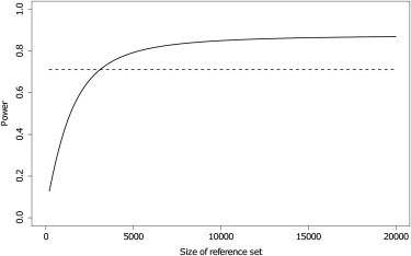
Effect of the Size of the Reference Set on the Power of the Two-Stage Procedure

Power of one-stage (dashed) and two-stage (solid) tests as the size of the reference set varies. MAF of the causal SNP: 0.25. Odds ratio of causal SNP, 1.3. 2000 cases, 3000 controls, 344087 null markers, ${\alpha }_1=0.025$.

On the other hand, diminishing returns means there is little advantage to going beyond 15,000 individuals in the reference set. For smaller or larger reference sets, one can vary the value of ${\alpha }_1$ to maximize the power of the two-stage approach. Table 4 shows the optimal value of ${\alpha }_1$ for different reference set sizes if the power to detect a variant with frequency 0.25 and odds ratio 1.3 is to be maximized. Note that ${\alpha }_1$ = 1 will reduce the two-stage procedure to the traditional one-stage test but give the same power.

Table 4.

Optimal Values of α₁ for Different Sizes of the Reference Set

Size of Reference Set	Optimal α1	Power of Two-Stage Approach
1,000	1	0.714
2,500	0.304	0.747
5,000	0.1	0.803
10,000	0.036	0.852
15,000	0.022	0.873
20,000	0.018	0.885

MAF of the causal SNP: 0.25. Odds ratio of the causal SNP: 1.3. There were 2,000 cases, 3,000 controls, and 344,087 null markers.

In Figure 4 we show how the power of the two-stage approach depends on the significance level used in the first stage. The power increases sharply to a maximum and then decreases gradually. For this particular set of parameters, the optimal significance level is 0.0143, but this will differ according to the odds ratio, MAF, and number of SNPs being tested. It is interesting to note that the power decreases gradually as ${\alpha }_1$ increases, so the two-stage approach is quite robust to the choice of ${\alpha }_1$ so long as it is sufficiently high.

Figure 4.

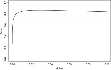
Effect of the First-Stage Significance Level on the Power of the Two-Stage Procedure

Power of one-stage (dashed) and two-stage (solid) procedure as the first-stage significance level varies. MAF of the causal SNP: 0.25. Odds ratio of the causal SNP: 1.3. There were 2,000 cases, 3,000 controls, a reference panel of 12,000 individuals, and 344,087 null markers.

Power when Reference and Test Populations Differ

When the reference population is different from the test population, the postulated allele frequencies will no longer match the frequencies in the controls. This will affect both the number of null markers being tested at the second stage and the probability that an associated marker will get through stage 1. We consider a uniform distribution of background allele frequencies between 0.05 and 0.5, as well as control and reference frequencies that follow the Balding-Nichols model described in the Material and Methods. Table 5 shows the expected number of null markers at the second stage, as well as the power of the one- and two-stage tests, for a series of values of the population separation $F_{ST}$.

Table 5.

Power Comparison when Reference and Control Populations Are Different

FST	E (m0)	First-Stage Power	Second-Stage Power	Overall Two-Stage Power	One-Stage Power
0	10,141	0.951	0.906	0.861	0.712
10−5	14,345	0.949	0.895	0.849	0.626
10−4	56,263	0.900	0.828	0.746	0.625
10−3	203,358	0.727	0.748	0.554	0.623
10−2	303,153	0.794	0.701	0.564	0.606
10−1	338,330	0.932	0.571	0.527	0.506

Power of one- and two-stage test procedures as a function of separation $F_{ST}$ between sample and reference populations. $E\left(m_0\right)$: expected number of markers carried forward from stage 1.

Table 5 shows that as $F_{ST}$ increases, the expected number of null SNPs getting through to the second stage increases rapidly. As a result, the multiple test correction applied at the second stage increases and the second-stage power decreases monotonically. On the other hand, the first-stage power decreases monotonically and then increases again. This seems surprising, but it occurs because the power function of the first stage is not symmetric in the MAF around the background value. This result also assumes that the odds ratio does not vary with the control MAF. The two-stage analysis remains more powerful than the one-stage analysis for values of $F_{ST}$ less than 10⁻³, which is the order of magnitude of separation between populations within Europe. It is clearly important that the reference population be a close match to the sample at hand.

Power when Reference Sample Is Unscreened for Disease

Another scenario that leads to different MAFs between the control and the reference samples is when the controls are screened to be free of disease but the reference set is unscreened. The result of this will be that the frequency in the reference set is a weighted sum of the frequency in screened controls and the frequency in cases; the weight will depend on the disease prevalence. Again, the difference between the postulated and actual allele frequencies will increase the number of null markers tested in the second stage and affect the power but not the type 1 error rate.

The degree to which this factor affects the power will depend on the prevalence of the disease. If the phenotype is rare, then the reference set will consist mostly of unaffected individuals, and the MAF will be close to that of the controls. If the phenotype is more common, the power of the first stage can be severely affected. Figure 5 shows the power of the two-stage test procedure as the prevalence of the disease changes for ${\alpha }_1$ = 0.025, population MAF = 0.25, odds ratio = 1.3, and other parameters as before. Note that the prevalence does not change the MAF of the screened controls, so the power of the one-stage test procedure is constant.

Figure 5.

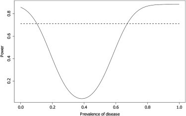
Effect of Disease Prevalence on the Power of the Two-Stage Procedure

Power of one-stage (dashed) and two-stage (solid) test statistics when controls are screened and reference-set individuals are not and as the prevalence of the disease varies. MAF of the causal SNP: 0.25. Odds ratio of the causal SNP: 1.3. There were 2,000 cases, 3,000 controls, a reference panel of 12,000 individuals, and 344,087 null markers. ${\alpha }_1=0.025$.

Figure 5 shows that this factor can lead to a disastrous loss of power when the disease prevalence is high. The power is at its lowest when the prevalence is close to 0.4, which is also the proportion of cases in the sample. In fact, for the above parameters, the formula in Equation 5 gives the minimum power at a prevalence of 0.386. We see that, similar to the exact result we obtained for linear regression, the first stage has no power when the case sampling fraction is close to (although not exactly equal to) that achieved under random ascertainment.

Analysis of WTCCC Data

We analyzed each of the seven diseases in the WTCCC data by using the other six sets of cases as an external reference panel. Table 6 shows the total number of significant SNPs in each disease. There is variation in the relative performance of one- and two-stage analyses, but over all seven diseases there is a higher total of significant associations from the two-stage analysis. Among SNPs that were not nominally significant in stage 2, the stage 1 and 2 statistics were uncorrelated, as expected.

Table 6.

Numbers of Genome-wide Significant SNPs in One- and Two-Stage Analysis of the WTCCC Data

Disease	One-Stage	Two-Stage	Size Stage 1	Size Stage 2	Correlation
BD	2	1	341,890	11,824	0.0065
CAD	20	10	345,460	10,477	−0.0009
CD	68	72	345,628	11,199	0.008
HT	3	2	343,615	10,085	−0.0045
RA	174	165	343,672	11,087	0.0021
T1D	471	500	344,684	11,372	0.0024
T2D	18	34	343,658	11,065	0.0011
Total	756	784

Abbreviations are as follows: BD, bipolar disorder (BPAD; [MIM 125480]); CAD, coronary artery disease; CD, Crohn disease (CD; [MIM 266600]); HT, hypertension (HTN; [MIM 145500]); RA, rheumatoid arthritis (RA; [MIM 180300]); T1D, type-1 diabetes (T1DM; [MIM 222100]); and T2D, type-2 diabetes (NIDDM; [MIM 125853]). Numbers include SNPs that passed initial quality control but were later discarded after inspection of cluster plots. Size stage 1: the number of SNPs included in the first stage. Size stage 2: the number of SNPs carried forward into the second stage. Correlation: correlation between stage 1 and stage 2 statistics for SNPs with p > 0.05 in stage 2.

There were eight regions that were significant in the two-stage but not the one-stage analysis; they are summarized in Table 7. Each of the regions has been subsequently validated in an independent GWAS or a meta-analysis. The regions were slightly short of significance in the one-stage analysis, but all bar one had been marked as suggestive in the WTCCC paper. Because of the reduced multiplicity in the second stage (equivalently, the increased prior odds), these markers became genome-wide significant under our approach. We computed an adjusted p value for each of these markers by multiplying the stage 2 p value by the ratio of the number of markers in stage 2 to the number in stage 1. This gives a p value that is calibrated against the initial prior odds, and as such it can be directly compared to the p value from a one-stage analysis. Table 7 shows that the adjusted p values are genome-wide significant when the one-stage p values are not.

Table 7.

Regions that Were Genome-wide Significant in Two-Stage Analysis but Not in One-Stage Analysis

Disease	Chromosome	Lead SNP	Mb	Stage 2	Adjusted Stage 2	WTCCC	Case Frequency	Control Frequency	Reference Frequency	Other WTCCC	Replication
CD	3	rs9858542	49.68	7.23 × 10−7	2.19 × 10−8	7.71 × 10−7	0.330	0.282	0.285	Genotypic test, expanded controls	Franke31
CD	6	rs7768538	32.84	1.76 × 10−6	5.34 × 10−8	8.65 × 10-7a	0.412	0.463	0.468		Franke
CD	21	rs2836754	39.21	1.04 × 10−5	3.15 × 10−8	n/a	0.399	0.353	0.352	Expanded controls	Frankeb
RA	6	rs5029939	138.24	8.48 × 10−6	2.74 × 10−7	4.99 × 10-6 [a]	0.055	0.036	0.035		Stahl32
T1D	10	rs10795791	6.15	1.16 × 10−5	3.81 × 10−7	7.96 × 10−6	0.456	0.411	0.414	Expanded controls	Barrett33
T2D	2	rs6718526	161.04	3.06 × 10−6	9.85 × 10−8	2.4 × 10−6	0.171	0.209	0.205	Expanded controls	Qi34
T2D	6	rs9465871	20.83	5.69 × 10−6	1.83 × 10−7	1.00 × 10-6a	0.218	0.178	0.182	Genotypic test	Zeggini35
T2D	12	rs1495377	69.86	1.47 × 10−6	4.73 × 10−8	1.31 × 10−6	0.547	0.497	0.502	Expanded controls	Zeggini

Disease abbreviations are as in Table 6. Stage 2: p value from allelic Wald test in the second stage. Adjusted stage 2: p value from stage 2 multiplied by the ratio of the number of SNPs in stage 2 to the number in stage 1. WTCCC: p value from trend test reported in WTCCC paper. Case frequency: allele frequency in the cases. Control frequency: allele frequency in the controls. Reference frequency: allele frequency in the combined cases of the other six diseases. Other WTCCC: other tests performed in the WTCCC study in which the SNP had genome-wide significance. Replication: source of subsequent validation of this association.

^ap value for a different SNP in the same region.

^bReplication was 5 Mb from this SNP.

There were three regions that were significant in the one-stage but not the two-stage analysis; they are summarized in Table 8. Here, the regions were eliminated in the first stage, even though the second-stage analysis was genome-wide significant. These regions, too, have been subsequently validated, so that they represent false negatives of the two-stage analysis. Two of these might be due to a shared genetic basis between inflammatory bowel disease (IBD; [MIM 266600]) and type-1 diabetes (T1DM; [MIM 222100]); rs2542151 has been independently associated with T1DM,²⁷ and rs17388568 has been independently associated with ulcerative colitis (UC; [MIM 191390]).²⁸ In all three cases the reference frequencies are closer to the case frequency than to the control frequency, reducing the significance of the stage 1 test.

Table 8.

Regions that Had Genome-wide Significance in the WTCCC Study but Not in the Two-Stage Analysis

Disease	Chromosome	Lead SNP	Mb	Stage 1	Case Frequency	Control Frequency	Reference Frequency	Replication
CD	5	rs1000113	150.22	0.74	0.098	0.067	0.076	Franke31
CD	18	rs2542151	12.77	0.22	0.209	0.163	0.173	Franke
T1D	4	rs17388568	123.69	0.44	0.307	0.260	0.283	Barrett33

Stage 1: p value from first stage analysis. Case frequency: allele frequency in the cases. Control frequency: allele frequency in the controls. Reference frequency: allele frequency in the combined cases of the other six diseases. Replication: source of subsequent validation of this association.

Discussion

We have given a general description of two-stage analysis of GWAS data; this analysis includes previously developed applications to family-based association and gene-environment interaction testing. With regard to the former, we recover previous work exactly, whereas for the latter we obtain an alternative approach. In both cases our formulation offers new insights and potential advantages over previous methods. Our general description opens up a range of possible further applications. It can be applied to any analysis that both involves testing a normally distributed parameter estimator and depends on a nuisance parameter for which a reasonable value can be postulated. This includes many common parametric and semiparametric models. We have considered semiparametric formulations of linear and logistic regression and have shown that if the population mean is used as a postulated value of the intercept, then two-stage analysis can offer increased power if there is selection on the independent variables. This approach might therefore hold promise for studies such as recall-by-genotype phenome scans, comparisons of disease-selected and -unselected subjects, and case-control studies of rare disease. It could also be applicable to analysis of secondary quantitative traits in case-control samples, although the appropriate specification of a postulated nuisance parameter is not obvious and is left to future work.

Focusing on standard case-control studies, we propose a first-stage statistic that incorporates an external estimate of the allele frequency. We have shown that if MAFs in the external reference set have the same underlying mean as those in the controls, then there is scope for a significant gain in power via the two-stage approach. This condition requires that the reference set and controls be from the same population and that either the disease is rare or both sets be unscreened (or both be screened) for the disease. As the separation between the populations increases, the power gain rapidly diminishes and becomes a power loss when the separation is greater than that typically found between European populations. Furthermore, if the controls are screened for disease and the reference individuals are unscreened, then the power can be severely diminished for certain values of the disease prevalence. The size of the reference set and the sample at hand also need to be of similar sizes, so resources such as the HapMap and 1000 Genomes databases may not be sufficient. Although these factors might seem like significant drawbacks, the sheer number of datasets becoming available makes it likely that several suitable reference sets will be possible for each case-control study.

In principle, our approach can be applied with summary data only and does not require individual subject data. However, if covariates are included in the model, as is often done as a means of controlling for population stratification, then individual data will be needed. There is no problem in principle with applying our approach with covariates because we can simply test our parameters after including covariates in the model. It might be necessary to rescale or recode covariates so that the external reference value corresponds to a parameter in the model, for example the MAF in a particular sub-population. The allowance for covariates is another advance on previous methods.

Of course, greater improvements in power are possible from a joint analysis of the two stages when the assumption in the first stage is explicitly controlled for.^4,29 This was done in the WTCCC study, when cases from clinically distinct diseases were pooled with the controls so that the total sample size increased. These “expanded controls” analyses detected some, but not all, of the additional associations we found via two-stage analysis. However, our aim is to show the utility of external summary data, when available, while retaining robustness to a mismatch between the external data and the sample at hand. We expect that reference databases of allele frequencies will become available without the individual genotypes that would allow statistical methods to adjust for population differences between reference and sample data. We aim to show how these data can improve standard GWAS analysis without incurring bias.

Our WTCCC analysis is the first application of two-stage analysis to multiple datasets and confirms the higher power of this approach. We detected eight true positives that were missed by standard analysis. Although our two-stage analysis missed three associations that were detected by standard methods, two of these can be attributed to the choice of reference panel, which includes cases from related diseases, a situation that need not occur in general.

Two-stage approaches have been described as “screening” followed by “replication.”^4,7,9 We discourage this usage because, in our view, replication involves confirming a specific hypothesis that has already been firmly established. In contrast, the first of our two stages merely selects a subset of markers and does not formally generate hypotheses for testing. However, we have noted that the evidence for association is modified to a degree by the first stage, to which the second is adaptive in its adjustment for multiplicity.

Bayesian methods offer an alternative approach to including assumed values of model parameters but still allowing for uncertainty in the assumptions.³⁰ At one extreme, an uninformative prior distribution on the nuisance parameter corresponds to a one-stage analysis, whereas at the other, a highly informative prior distribution corresponds to a joint analysis of the two stages. In the situations we have considered, we can expect the stage 1 assumptions to hold for some markers and not for others. A prior distribution that reflects this property and correctly models departures from the assumption should lead to a more powerful analysis than our two-stage approaches. Our methods are a compromise that improves power by including prior information on nuisance parameters while retaining robustness to mis-specification of that information. In this respect, two-stage and Bayesian analyses are alternative approaches that offer different advantages according to context.

In practice, standard one-stage analyses are unlikely to be discarded even if more powerful alternatives are available. However, we think that two-stage analysis should join the array of complementary methods that can be applied after initial simple analyses are completed. We have given a general account of this approach, as well as its advantages and limitations, and hope that this will stimulate its further study and use in a wider range of applications.

Appendix A

Effect of Prevalence on Power in Case-Control Studies

In terms of the allele frequencies p₀ and p_1, the number of controls and cases n₀ and n₁, and the prevalence q₀, the expectation of the stage 1 statistic is

$$\log \left(\frac{p_1\left(1-p_0\right)}{\left(1-p_1\right)p_0}\right)+\left(1+\frac{n_0}{n_1}\right)\log \left(\frac{p_0\left(1-q_0{p}_1-\left(1-q_0\right)p_0\right)}{\left(1-p_0\right)\left(q_0{p}_1+\left(1-q_0\right)p_0\right)}\right).$$

Therefore, the value of q₀ that gives mean 0 solves the following equation:

$$\log \left(\frac{q_0{p}_1+\left(1-q_0\right)p_0}{1-q_0{p}_1-\left(1-q_0\right)p_0}\right)=\nu \log \left(\frac{p_1\left(1-p_0\right)}{\left(1-p_1\right)p_0}\right)+\log \left(\frac{p_0}{\left(1-p_0\right)}\right),$$

where $v={\left(1+n_0/n_1\right)}^{-1}$. Then

$$\left(\frac{q_0{p}_1+\left(1-q_0\right)p_0}{1-q_0{p}_1-\left(1-q_0\right)p_0}\right)={\left(\frac{p_1}{1-p_1}\right)}^v{\left(\frac{p_0}{1-p_0}\right)}^{1-v}\equiv \tilde{p},$$

and therefore $\tilde{p}/1+\tilde{p}=q_0{p}_1+\left(1-q_0\right)p_0$, giving $q_0=\tilde{p}{\left(1+\tilde{p}\right)}^{-1}-p_0/p_1-p_0$.

Web Resources

The URL for data presented herein is as follows:

• Online Mendelian Inheritance in Man (OMIM), http://www.omim.org

References

- 1.Lee S.H., Wray N.R., Goddard M.E., Visscher P.M. Estimating missing heritability for disease from genome-wide association studies. Am. J. Hum. Genet. 2011;88:294–305. doi: 10.1016/j.ajhg.2011.02.002. [DOI] [PMC free article] [PubMed] [Google Scholar]
- 2.Lango Allen H., Estrada K., Lettre G., Berndt S.I., Weedon M.N., Rivadeneira F., Willer C.J., Jackson A.U., Vedantam S., Raychaudhuri S. Hundreds of variants clustered in genomic loci and biological pathways affect human height. Nature. 2010;467:832–838. doi: 10.1038/nature09410. [DOI] [PMC free article] [PubMed] [Google Scholar]
- 3.Satagopan J.M., Venkatraman E.S., Begg C.B. Two-stage designs for gene-disease association studies with sample size constraints. Biometrics. 2004;60:589–597. doi: 10.1111/j.0006-341X.2004.00207.x. [DOI] [PMC free article] [PubMed] [Google Scholar]
- 4.Skol A.D., Scott L.J., Abecasis G.R., Boehnke M. Joint analysis is more efficient than replication-based analysis for two-stage genome-wide association studies. Nat. Genet. 2006;38:209–213. doi: 10.1038/ng1706. [DOI] [PubMed] [Google Scholar]
- 5.Wu J., Devlin B., Ringquist S., Trucco M., Roeder K. Screen and clean: A tool for identifying interactions in genome-wide association studies. Genet. Epidemiol. 2010;34:275–285. doi: 10.1002/gepi.20459. [DOI] [PMC free article] [PubMed] [Google Scholar]
- 6.Millstein J., Conti D.V., Gilliland F.D., Gauderman W.J. A testing framework for identifying susceptibility genes in the presence of epistasis. Am. J. Hum. Genet. 2006;78:15–27. doi: 10.1086/498850. [DOI] [PMC free article] [PubMed] [Google Scholar]
- 7.Van Steen K., McQueen M.B., Herbert A., Raby B., Lyon H., Demeo D.L., Murphy A., Su J., Datta S., Rosenow C. Genomic screening and replication using the same data set in family-based association testing. Nat. Genet. 2005;37:683–691. doi: 10.1038/ng1582. [DOI] [PubMed] [Google Scholar]
- 8.Ionita-Laza I., McQueen M.B., Laird N.M., Lange C. Genomewide weighted hypothesis testing in family-based association studies, with an application to a 100K scan. Am. J. Hum. Genet. 2007;81:607–614. doi: 10.1086/519748. [DOI] [PMC free article] [PubMed] [Google Scholar]
- 9.Murphy A., Weiss S.T., Lange C. Screening and replication using the same data set: Testing strategies for family-based studies in which all probands are affected. PLoS Genet. 2008;4:e1000197. doi: 10.1371/journal.pgen.1000197. [DOI] [PMC free article] [PubMed] [Google Scholar]
- 10.Murcray C.E., Lewinger J.P., Gauderman W.J. Gene-environment interaction in genome-wide association studies. Am. J. Epidemiol. 2009;169:219–226. doi: 10.1093/aje/kwn353. [DOI] [PMC free article] [PubMed] [Google Scholar]
- 11.Kooperberg C., Leblanc M. Increasing the power of identifying gene x gene interactions in genome-wide association studies. Genet. Epidemiol. 2008;32:255–263. doi: 10.1002/gepi.20300. [DOI] [PMC free article] [PubMed] [Google Scholar]
- 12.Murcray C.E., Lewinger J.P., Conti D.V., Thomas D.C., Gauderman W.J. Sample size requirements to detect gene-environment interactions in genome-wide association studies. Genet. Epidemiol. 2011;35:201–210. doi: 10.1002/gepi.20569. [DOI] [PMC free article] [PubMed] [Google Scholar]
- 13.Zheng G., Song K., Elston R.C. Adaptive two-stage analysis of genetic association in case-control designs. Hum. Hered. 2007;63:175–186. doi: 10.1159/000099830. [DOI] [PubMed] [Google Scholar]
- 14.Wellcome Trust Case Control Consortium Genome-wide association study of 14,000 cases of seven common diseases and 3,000 shared controls. Nature. 2007;447:661–678. doi: 10.1038/nature05911. [DOI] [PMC free article] [PubMed] [Google Scholar]
- 15.Lake S.L., Blacker D., Laird N.M. Family-based tests of association in the presence of linkage. Am. J. Hum. Genet. 2000;67:1515–1525. doi: 10.1086/316895. [DOI] [PMC free article] [PubMed] [Google Scholar]
- 16.Abecasis G.R., Cardon L.R., Cookson W.O. A general test of association for quantitative traits in nuclear families. Am. J. Hum. Genet. 2000;66:279–292. doi: 10.1086/302698. [DOI] [PMC free article] [PubMed] [Google Scholar]
- 17.Dudbridge F. Likelihood-based association analysis for nuclear families and unrelated subjects with missing genotype data. Hum. Hered. 2008;66:87–98. doi: 10.1159/000119108. [DOI] [PMC free article] [PubMed] [Google Scholar]
- 18.Cordell H.J., Barratt B.J., Clayton D.G. Case/pseudocontrol analysis in genetic association studies: A unified framework for detection of genotype and haplotype associations, gene-gene and gene-environment interactions, and parent-of-origin effects. Genet. Epidemiol. 2004;26:167–185. doi: 10.1002/gepi.10307. [DOI] [PubMed] [Google Scholar]
- 19.Jones R., Pembrey M., Golding J., Herrick D. The search for genenotype/phenotype associations and the phenome scan. Paediatr. Perinat. Epidemiol. 2005;19:264–275. doi: 10.1111/j.1365-3016.2005.00664.x. [DOI] [PubMed] [Google Scholar]
- 20.Denny J.C., Ritchie M.D., Basford M.A., Pulley J.M., Bastarache L., Brown-Gentry K., Wang D., Masys D.R., Roden D.M., Crawford D.C. PheWAS: Demonstrating the feasibility of a phenome-wide scan to discover gene-disease associations. Bioinformatics. 2010;26:1205–1210. doi: 10.1093/bioinformatics/btq126. [DOI] [PMC free article] [PubMed] [Google Scholar]
- 21.Rose S., van der Laan M.J. Simple optimal weighting of cases and controls in case-control studies. Int. J. Biostat. 2008;4:19. doi: 10.2202/1557-4679.1115. [DOI] [PMC free article] [PubMed] [Google Scholar]
- 22.Purcell S., Neale B., Todd-Brown K., Thomas L., Ferreira M.A., Bender D., Maller J., Sklar P., de Bakker P.I., Daly M.J., Sham P.C. PLINK: A tool set for whole-genome association and population-based linkage analyses. Am. J. Hum. Genet. 2007;81:559–575. doi: 10.1086/519795. [DOI] [PMC free article] [PubMed] [Google Scholar]
- 23.Balding D.J., Nichols R.A. A method for quantifying differentiation between populations at multi-allelic loci and its implications for investigating identity and paternity. Genetica. 1995;96:3–12. doi: 10.1007/BF01441146. [DOI] [PubMed] [Google Scholar]
- 24.Altshuler D.M., Gibbs R.A., Peltonen L., Altshuler D.M., Gibbs R.A., Peltonen L., Dermitzakis E., Schaffner S.F., Yu F., Peltonen L., International HapMap 3 Consortium Integrating common and rare genetic variation in diverse human populations. Nature. 2010;467:52–58. doi: 10.1038/nature09298. [DOI] [PMC free article] [PubMed] [Google Scholar]
- 25.Dudbridge F., Gusnanto A. Estimation of significance thresholds for genomewide association scans. Genet. Epidemiol. 2008;32:227–234. doi: 10.1002/gepi.20297. [DOI] [PMC free article] [PubMed] [Google Scholar]
- 26.Won S., Wilk J.B., Mathias R.A., O'Donnell C.J., Silverman E.K., Barnes K., O'Connor G.T., Weiss S.T., Lange C. On the analysis of genome-wide association studies in family-based designs: a universal, robust analysis approach and an application to four genome-wide association studies. PLoS Genet. 2009;5:e1000741. doi: 10.1371/journal.pgen.1000741. [DOI] [PMC free article] [PubMed] [Google Scholar]
- 27.Cooper J.D., Smyth D.J., Smiles A.M., Plagnol V., Walker N.M., Allen J.E., Downes K., Barrett J.C., Healy B.C., Mychaleckyj J.C. Meta-analysis of genome-wide association study data identifies additional type 1 diabetes risk loci. Nat. Genet. 2008;40:1399–1401. doi: 10.1038/ng.249. [DOI] [PMC free article] [PubMed] [Google Scholar]
- 28.Anderson C.A., Boucher G., Lees C.W., Franke A., D'Amato M., Taylor K.D., Lee J.C., Goyette P., Imielinski M., Latiano A. Meta-analysis identifies 29 additional ulcerative colitis risk loci, increasing the number of confirmed associations to 47. Nat. Genet. 2011;43:246–252. doi: 10.1038/ng.764. [DOI] [PMC free article] [PubMed] [Google Scholar]
- 29.Macgregor S. Optimal two-stage testing for family-based genome-wide association studies. Am. J. Hum. Genet. 2008;82:797–799. doi: 10.1016/j.ajhg.2008.02.003. author reply 799–800. [DOI] [PMC free article] [PubMed] [Google Scholar]
- 30.Antonyuk A., Holmes C. On testing for genetic association in case-control studies when population allele frequencies are known. Genet. Epidemiol. 2009;33:371–378. doi: 10.1002/gepi.20375. [DOI] [PubMed] [Google Scholar]
- 31.Franke A., McGovern D.P., Barrett J.C., Wang K., Radford-Smith G.L., Ahmad T., Lees C.W., Balschun T., Lee J., Roberts R. Genome-wide meta-analysis increases to 71 the number of confirmed Crohn's disease susceptibility loci. Nat. Genet. 2010;42:1118–1125. doi: 10.1038/ng.717. [DOI] [PMC free article] [PubMed] [Google Scholar]
- 32.Stahl E.A., Raychaudhuri S., Remmers E.F., Xie G., Eyre S., Thomson B.P., Li Y., Kurreeman F.A., Zhernakova A., Hinks A., BIRAC Consortium. YEAR Consortium Genome-wide association study meta-analysis identifies seven new rheumatoid arthritis risk loci. Nat. Genet. 2010;42:508–514. doi: 10.1038/ng.582. [DOI] [PMC free article] [PubMed] [Google Scholar]
- 33.Barrett J.C., Clayton D.G., Concannon P., Akolkar B., Cooper J.D., Erlich H.A., Julier C., Morahan G., Nerup J., Nierras C., Type 1 Diabetes Genetics Consortium Genome-wide association study and meta-analysis find that over 40 loci affect risk of type 1 diabetes. Nat. Genet. 2009;41:703–707. doi: 10.1038/ng.381. [DOI] [PMC free article] [PubMed] [Google Scholar]
- 34.Qi L., Cornelis M.C., Kraft P., Stanya K.J., Linda Kao W.H., Pankow J.S., Dupuis J., Florez J.C., Fox C.S., Paré G., Meta-Analysis of Glucose and Insulin-related traits Consortium (MAGIC) Diabetes Genetics Replication and Meta-analysis (DIAGRAM) Consortium Genetic variants at 2q24 are associated with susceptibility to type 2 diabetes. Hum. Mol. Genet. 2010;19:2706–2715. doi: 10.1093/hmg/ddq156. [DOI] [PMC free article] [PubMed] [Google Scholar]
- 35.Zeggini E., Scott L.J., Saxena R., Voight B.F., Marchini J.L., Hu T., de Bakker P.I., Abecasis G.R., Almgren P., Andersen G., Wellcome Trust Case Control Consortium Meta-analysis of genome-wide association data and large-scale replication identifies additional susceptibility loci for type 2 diabetes. Nat. Genet. 2008;40:638–645. doi: 10.1038/ng.120. [DOI] [PMC free article] [PubMed] [Google Scholar]