Comprehensive analysis of the Cramer–Rao bounds for magnetic resonance temperature change measurement in fat–water voxels using multi-echo imaging

Abstract

Object

The aim of this paper is to characterize the noise propagation for MRI temperature change measurement with emphasis on finding the best echo time combinations that yield the lowest temperature noise.

Materials and methods

A Cramer–Rao lower-bound (CRLB) calculation was used to estimate the temperature noise for a model of the MR signal in fat–water voxels. The temperature noise CRLB was then used to find a set of echo times that gave the lowest temperature change noise for a range of fat–water frequency differences, temperature changes, fat/water signal ratios, and T2* values. CRLB estimates were verified by Monte Carlo simulation and in phantoms using images acquired in a 1.5 T magnet.

Results

Results show that regions exist where the CRLB predicts minimal temperature variation as a function of the other variables. The results also indicate that the CRLB values calculated in this paper provide excellent guidance for predicting the variation of temperature measurements due to changes in the signal parameters. For three echo scans, the best noise characteristics are seen for TE values of 20.71, 23.71, and 26.71 ms. Results for five and seven echo scans are also presented in the text.

Conclusion

The results present a comprehensive analysis of the effects of different scan parameters on temperature noise, potentially benefiting the selection of scan parameters for clinical MRI thermometry.

Introduction

To acquire more extensive thermometry in clinical heating applications, a number of research groups have demonstrated that magnetic resonance thermal imaging (MRTI) is effective and accurate for noninvasively assessing temperature changes in tissues associated with absorption of nonionizing radiation [1–7]. The most widely adopted MRTI method used to measure temperature changes is the proton resonant frequency shift (PRFS) method. The PRFS method measures changes in the proton resonance frequency of tissue (typically 0.01 ppm/°C in muscle [8]) and correlates it to temperature change. However, this method can have significant error in fatty tissues, such as the breast or liver. Since the fat frequency does not change compared to that of water, the PRFS change in a voxel depends on the fat to water (f/w) ratio, leading to errors if the f/w ratio is not taken into consideration.

Several methods have been proposed to deal with the errors caused by fat signal, including fat suppression [9–11], spectroscopy [12–14], and multi-echo fitting [15–17]. Multi-echo fitting methods (such as IDEAL [18]) have been used to create water-only images that can then be used to calculate temperature changes using normal PRFS techniques [15]. Other multi-echo methods directly fit for temperature change while accounting for the fat in the voxel [19]. While multi-echo fitting requires increased scan time and computation compared to fat suppression techniques, it provides the added benefit of fitting for the local magnetic (B₀) field. These field values can provide references for correction of field changes within both fat and water-rich tissue [20]. However, the effectiveness of these multi-echo techniques to fit for temperature change is heavily dependent on what echo times are sampled and the composition of the tissue. Experiments have been performed with phantoms, but only using echo times optimized for estimating the f/w magnitudes, not for temperature change.

Since accurate temperature measurement is needed for clinical applications, the intent of this study was to calculate echo times that optimize a multi-echo fitting method to obtain the minimum temperature change noise, i.e., we wish to maximize the temperature change signal-to-noise ratio. These values can be found using Monte Carlo simulations, but this can be time consuming, particularly given the parameter space examined in this paper. Alternatively, the Cramer–Rao lower bound (CRLB) can be used to theoretically calculate the temperature noise using much less computational time. The CRLB is the lower bound on the variance of an unbiased estimate [21,22]. An unbiased estimator is one in which the expected value of the variable (typically the mean) equals the true value.

CRLB analyses have been performed for multi-echo fitting techniques [17,23]. In the case of Li et al., a temperature noise CRLB value can be determined. While that work was a good demonstration of the usefulness of the CRLB in predicting temperature noise, it used a simple two-peak signal model, when many other studies have shown the need to account for the multiple peaks of fat in water-fat fitting experiments. As demonstrated in this study, the inclusion of multiple peaks of fat induces small changes in the temperature noise CRLB. However, these changes can be important when analyzing the temperature noise of a MR sequence for use in thermometry of hyperthermia. Previous studies also did not examine the relation between the CRLB and imaging parameters in detail, instead focusing solely on the first echo time.

In this study, a temperature noise CRLB model is developed that includes multiple fat peaks that is compared to a single-peak model. Additional parameters not previously investigated including the fat/water (f/w) ratio, T2* of water and fat, TE values of each echo, and the magnitude of temperature change are also investigated. The parameters were also examined concurrently, providing a more robust examination of their effects on the temperature noise. Finally, temperature noise measurements in fat–water phantoms were compared to the CRLB calculations. This was briefly investigated by Li et al., but with poor agreement for only one set of TE values. In this study, we aim to confirm the CRLB at many sets of TE values and use the multi-peak CRLB to provide good agreement between expected and measured temperature noise.

Background and theory

Our water and fat model contained three fat peaks such that the MR signal from a voxel containing both water and fat would be:

$$\begin{array}{cc}\hfill s\left(n\right)=& \left(A_{\text{water}}{e}^{\frac{-\mathrm{TE}\left(n\right)}{\mathrm{T}{2}_w^{\ast }}}{e}^{2\pi i\alpha f_0\mathrm{TE}\left(n\right)\Delta T}\right)\hfill \\ \hfill +& A_{\text{fat}}{e}^{\frac{-\mathrm{TE}\left(n\right)}{\mathrm{T}{2}_{\mathrm{f}}^{\ast }}\left({\beta }_1{e}^{2\pi \mathrm{iTE}\left(n\right)\Delta f_{\mathrm{fw}1}}+{\beta }_2{e}^{2\pi \mathrm{iTE}\left(n\right)\Delta f}fw2+{\beta }_3{e}^{2\pi \mathrm{iTE}\left(n\right)\Delta f}fw3\right)}\hfill \\ \hfill \times & e^{2\pi \mathrm{iTE}\left(n\right)\Psi }+\epsilon \hfill \end{array}$$ (1)

where A_water and A_fat are the TE = 0 (complex valued) amplitudes at the TR of interest for water and fat, respectively. $\mathrm{T}{2}_{\mathrm{w}}^{\ast }$ and $\mathrm{T}{2}_{\mathrm{f}}^{\ast }$ are the T2* values for water and fat, respectively, α is the PRFS thermal coefficient (0.01 ppm/°C), f₀ is the imaging frequency at 1.5 T (63.87 MHz), Δf_fw are the frequency differences between the fat peaks and the water peak at a “baseline” temperature, T_b, ψ is the offset from the imaging frequency (magnetic field inhomogeneity affecting both fat and water in a voxel), and ε is Gaussian noise with mean = 0 and variance = ${\sigma }_{\epsilon }^2$. β is the relative ratio of the area of each fat peak=compared to the area of all fat peaks combined, with all values adding up to 1. The echo number is n, for which there are a total of N echo times, ie, n = 1, 2,…, N. The set of echoes described by s(n) is referred to as an Echo Sampling Group (ESG). Finally, ΔT is the temperature change from the baseline temperature at which the fat–water frequency differences φ_fw would be measured. Theoretically, absolute temperature can be measured by fitting for ΔT for a known set of T_b and φ_fw, giving the measured temperature T = T_b + ΔT. While many groups have used single-peak model for fat, a number of reports have demonstrated the improvements in water-fat image separation gained by using a multi-peak representation of fat [24,25].

A matrix representation of the signal in Eq. 1 was derived and used to find the Fisher Information Matrix (FIM) using methods described by Pineda et al. [23]. These derivations can be found in the “Appendix”. The temperature variance calculated from the CRLB was obtained by calculating the diagonal elements of the FIM. This variance is valid for cases involving the calculation of temperature change (ΔT) from one set of TE images. However, in this study we assume that any given ΔT will need to have a baseline ΔT_b subtracted, and thus measurements at two time points were used to calculate temperature change. Thus, the temperature variance CRLB was calculated twice, with the first calculation having zero temperature change (but subject to noise) and the second calculation having a nonzero temperature change (also subject to noise) but with all other parameters the same. The variance was then converted to a standard deviation to provide a conventional expression of the error. This standard deviation is referred to as the temperature noise CRLB.

Materials and methods

Parameterization of echo times

For ease of notation, the echo times used were parameterized with three variables, all related to the phase angle between the water and fat signals. The starting angle is the angle between water and fat at the first TE value. The separation angle is the angle between water and fat that is added to the starting angle for each subsequent TE value. Lastly, the rotation number is how many full 360° rotations have occurred between water and fat phases before the starting angle. The equation used to calculate the TE values is shown below in Eq. 2.

$$\mathrm{TE}\left(\mathrm{n}\right)=\frac{\left(\text{rotation}+\frac{\text{starting angle}+(n-1)\ast \text{separation angle}}{360}\right)}{{\phi }_{\mathrm{fw}1}}$$ (2)

For all the TE values in this paper, the φ_fw1 was assumed to be 222 Hz (bulk methylene peak of fat at 1.5 T). A diagram illustrating the relationship between these three variables and the phase angle between water and fat is shown in Fig. 1.

Fig. 1.

Diagram explaining the parameterization of the phase difference between the water and fat signals each TE value of an ESG

Comparison of the temperature noise CRLB calculation with Monte Carlo simulation

Temperature noise CRLB values were compared to Monte Carlo simulation results to provide a check on the accuracy of the CRLB calculations. Because the simulation calculation time is quite long for a single set of parameters, only a limited range of parameters was investigated. An iterative nonlinear fitting algorithm based on the Levenberg-Marquardt fitting method was used to fit for A_water, A_fat, temperature change, and field offset directly by assuming that the signal is described by s(n) (Eq. 1 above). The algorithm, referred to as NLM-Temp, was programmed in Matlab (The Mathworks, Inc., Natick, MA), and each fit was allowed to iterate until it converged to a stable solution.

In the Monte Carlo calculation, for each of a number of ESGs, the NLM-Temp algorithm was used to calculate temperature, field offset, A_water, and A_fat for 5,000 sets of simulated data each with a different set of noise values for a given ESG with A_water = 5, A_fat = 5, $\mathrm{T}{2}_{\mathrm{w}}^{\ast }=\mathrm{T}{2}_{\mathrm{f}}^{\ast }=40\mathrm{ms}$, field offset ψ = −12.5 Hz, and ${\sigma }_{\epsilon }^2=0.5$ (SNR = 20 at TE = 0). A three-peak model for the fat was assumed with one peak at 1.22 ppm (222 Hz at 63.85 MHz), one at 1.96 ppm (175 Hz at 63.85 MHz), and the other at 5.22 ppm (−33 Hz at 63.85 MHz). The relative ratios (β) of each peak were 0.82, 0.11, and 0.07, respectively (based on measured ratios of fat peak areas taken from single voxel MR spectroscopy of the peanut oil used in our actual phantoms). The standard deviation of the calculated temperature was compared to the CRLB values calculated with the same signal values. The simulation was conducted for ESGs generated for five starting angles (60°, 120°, 180°, 240°, 300°) and for separation angles from 1° to 360° incremented by 5°. The mean of the simulated results were also calculated to compare with the correct variable value to check for areas of bias of the NLM-Temp algorithm.

Investigation of the temperature noise CRLB of fat–water signals for various effects

As shown in the results section, the Monte Carlo simulations confirmed the accuracy and regions of applicability of the temperature noise CRLB method. We made use of the computational efficiency of the temperature noise CRLB method to investigate a wide range of factors that could affect the temperature measurement error. For all calculations (unless otherwise noted), φ_fw1 = − 222 Hz, φ_fw2 = − 175 Hz, and φ_fw3 = − 33 Hz, the ratios of each peak were β₁ = 0.82, β₂ = 0.11 and β₃ = 0.07, rotation = 4 (see below), SNR = 1, A_water/A_fat = 1. $\mathrm{T}{2}_{\mathrm{w}}^{\ast }=40\mathrm{ms}$, $\mathrm{T}{2}_{\mathrm{f}}^{\ast }=25\mathrm{ms}$, and ΔT = 10°C. A SNR of 1 was chosen to allow scaling of the results in this paper to other SNR values. Since the temperature noise CRLB standard deviation scales linearly with input noise, the standard deviation of other situations can be obtained by dividing the values in this paper by the input SNR of a given setup. The following scenarios were investigated.

Single-peak versus multi-peak CRLB models

• CRLB values for single-peak and multi-peak lipid models were compared at the same ESGs

Examination of T2* effects

• One ESG was selected for a range of rotation from 0 to 30.

• Starting and separation angles were held constant at 150° yielding a range of TE = 1.9–137 ms as the rotation increased.

• $\mathrm{T}{2}_{\mathrm{w}}^{\ast }$ was kept constant at 40 ms, $\mathrm{T}{2}_{\mathrm{f}}^{\ast }$ was studied for values of 20, 40, and 60 ms.

• Based on a minimum noise value found near rotation = 4, all other simulations (below) used a rotation = 4 parameter to investigate the best case region.

Effect of starting TE and TE spacing

• Performed to gauge effect of uniform or non-uniform echo spacing on ΔT.

• Uniform TE spacing was tested by varying starting and separation angles from 1° − 360°, stepping by 1°, at a rotation of 4.

• Non-uniform TE spacing was tested by varying starting and separation angles Φ₂ and Φ₃ (see Fig. 1) from 1° − 360°, stepping by 1°C, independently at a rotation of 4.

• Comparisons were made within and between the uniform and non-uniform results.

Effect of fat–water frequency difference

• Performed based on report by McDannold et al. of frequency difference in breast between water and bulk methylene peaks from 3 to 3.75 ppm (190–240 Hz at 1.5 T) [26].

• Three φ_fw1 values were used: 202, 212, and 222 Hz.

• Starting and separation angles were varied from 1° − 360°, stepping by 1°, at a rotation of 4.

• Relative fat frequency offsets were preserved (φ_fw1 − φ_fw2 = −47 Hz and φ_fw1 − φ_fw3 = −255 Hz).

• ΔT was incremented from 0 to 20°C in increments of 5°C for φ_fw1 = 222 Hz.

Effect of fat/water signal ratio

• Performed due to variability of fat/water ratio in various areas of the body.

• Initially, starting and separation angles were varied from 1° − 360°, stepping by 1°, at a rotation of 4 for various f/w ratios.

• Based on equivalent noise changes for varying f/w ratios, an in-depth study was performed on just one starting/separation angle pair.

• Starting and separation angles were set to 150°, rotation 4, while the f/w ratio was adjusted from 1 to 99% fat signal in increments of 1%.

Combined effect of fat–water frequency difference, fat/water ratio, and temperature change

• Performed to find an “overall” optimized ESG that would minimize the noise variations seen when each of these three parameters were considered together.

• Starting and separation angles were varied from 1° − 360°, step 1°, at a rotation of 4.

• φ_fw1 values were varied from 190–240 Hz, in 1 Hz increments.

• Relative fat frequency offset were preserved (φ_fw1−φ_fw2 = −47 Hz and φ_fw1 − φ_fw3 = −255 Hz).

• f/w signal ratios were varied from 10–90% fat, in increments of 10%.

• ΔT was varied from 0° − 15°C in 5° increments.

• The standard deviation of all CRLB values for a given ESG was calculated to find the ESG(s) that had minimum noise variation due all the permutations performed for the ESG.

Effect of number of echoes used

• Number of echoes were varied from 3 – 15.

• Starting and separation angles were varied from 1° − 360°, step 1°, at a rotation of 4.

Heating and temperature noise measurement in fat/water phantoms

Phantom construction, spectral and fat/water composition determination

Phantom measurements were compared to the theoretical temperature noise CRLB calculations. Additionally, the phantoms were heated to confirm the effectiveness of the method at measuring temperature change accurately. Three different oil-in-water gelatin phantoms were constructed, each using the recipe described in Soher et al. [15] as modified from Madsen et al. [27] Peanut oil was used due to its use in previous papers [24] to mimic body fat and has a well-documented spectrum. The phantoms were made with different f/w concentrations, with volume ratios of 70:30, 50:50, and 30:70 water to fat. The first two phantoms were contained in 12.7-cm-diameter HDPE cylinders of 25.4 cm length, while the 30:70 phantom was contained in a 10.8-cm-diameter PVC cylinder of 17.8 cm length (the smaller volume was needed to create a homogenous phantom of this composition). Four catheters were inserted along the length of each phantom, one at the center of each cylinder and three near the outside edge of the phantom at 120° offsets from each other. The catheters allowed the insertion of fluoroptic temperature probes (Lumasense Technologies, Santa Clara, CA) to measure absolute temperature inside the phantom.

The frequencies and relative amplitude ratios of the fat peaks were measured using single voxel, short echo time MR Point Resolved Spectroscopy (PRESS) to determine fat peak frequency values and relative amplitude ratios. Acquisition parameters were TR = 5s, TE = 30 ms, SW = 2,000 Hz, 2,048 points, and 8 averages with no water suppression. PRESS voxels were acquired from 1 cm³ voxels centered at each of the catheter locations midway along the length of each phantom to determine the homogeneity of each solution. The SITools-FITT software package [28] was used to fit areas and frequencies beneath a single water peak, and six lipid peaks (Fig. 2). The scanning was performed on a 3 T Trio MR scanner (Siemens Medical Systems, Erlangen, Germany).

Fig. 2.

a PRESS spectra at the center of each phantom. b Fits to six spectral lines of the 50:50 spectrum

Data were also acquired for fitting of the A_water, A_fat, $\mathrm{T}{2}_{\mathrm{w}}^{\ast }$, and $\mathrm{T}{2}_{\mathrm{w}}^{\ast }$ values. Images of the phantoms were acquired for nine 3-echo ESGs chosen with a varying starting angles and a separation angle of 120°. TE parameters for these ESGs are shown in Table 1. TE values ranged from 6.3 to 31.7 ms. The parameters in Table 1 were chosen to enable robust fitting of the T2* and amplitude values of both the fat and water signals. Images were acquired from a 1-cm-thick slice on a 1.5 T GE Signa HDX (General Electric, Milwaukee, WI) with a 2D axial SPGR sequence with TR = 51 ms, flip angle = 30°, BW = 15.6kHz, FOV = 24 cm, 128× 128, and NEX = 2.0.

Table 1.

TE parameters for the MP-IDEAL ESGs

Rotation	Starting angle	Separation angle
1	150	120
2	165	120
3	125	120
3	190	120
3	310	120
4	120	120
4	190	120
5	135	120
6	135	120

The nine 3-echo ESG images were processed with an offline implementation of the multi-peak IDEAL (MP-IDEAL) algorithm described by Yu et al. [24]. The A_water, A_fat, $T{2}_{\mathrm{w}}^{\ast }$, and $\mathrm{T}{2}_{\mathrm{f}}^{\ast }$ values of each phantom were fit using a nonlinear Levenberg-Marquardt algorithm that used the nine water and fat images resulting from the IDEAL separation. All of these calculations were performed in Matlab. Referring to Fig. 2b, only peaks 1, 4, and 5 were included. Peak 3 was combined with peak 4 and peak 6 was combined with peak 5. Peak 2 was ignored due to its small amplitude. These adjustments were made to simplify the MP-IDEAL calculations.

Phantom heating experiment

All three phantoms were heated using a mini-annular phased array (MAPA) RF applicator with four antennas. Data were acquired similarly to the work in Soher et al on a 1.5 T Signa HDX. Three echo and five echo ESGs were acquired before, during, and after RF heating was applied. Both ESGs were acquired with rotation = 3, starting angle 261°, and separation angle = 245° (corresponding to TEs = of 16.78, 19.84, 22.91, 25.98, 29.04 ms for the 5-echo ESG). The complex image data from the ESGs was processed with the NLM-Temp algorithm to find the temperature changes. The initial guess for the A_water, A_fat, T2*, and fat peak area values were based on values from the MP-IDEAL measurements in the phantom composition analysis. The difference between the temperature at the first time point was subtracted from the temperature at all other time points to provide referenced temperature measurement. MR temperature measurements were then compared to the fluoroptic probe measurements that were recorded every 10 s for the duration of the experiment. Additionally, temperature noise was calculated by measuring the standard deviation of the temperature in each pixel across the first nine time points (before heat was applied). These calculations were performed for each pixel around the catheters and then averaged. These averaged values were then compared to a temperature noise CRLB values calculated using the values from the phantom composition analysis and the SNR of the images.

Temperature noise measurements—without heating

Phantom comparisons to theoretical CRLB and Monte Carlo estimates were performed using several selected TE spacing combinations that distinctly illustrate different noise behavior seen in the calculations. Phantoms were allowed to reach equilibrium with the MR scanner room temperature overnight and were scanned using the standard GE CP head coil. Fluoroptic temperature probes (Lumasense Technologies, Santa Clara, CA) were inserted into each of four catheters in the phantom and centered in the slice of interest. Temperature data were acquired from each probe every 10 s during the experiment. MR scan parameters were the same as those used above for the phantom composition measurements. ESGs were acquired for 3-echo, 5-echo, and 7-echo combinations using the same SPGR sequence used for the MP-IDEAL measurements. The starting angle and separation angles of each ESG are shown in Table 2 (also indicated by asterisks in Fig. 5). Each ESG was acquired six times consecutively, to allow for referenced temperature imaging and averaging of the results. No heat was applied to the phantom to provide homogenous regions of the phantom where standard deviation measurements could be acquired without error due to spatial distributions of heat, since any variation in the heat distribution could result in large errors in the noise measurement.

Table 2.

TE parameters for the ESGs to confirm the temperature noise CRLB values

3-echo				5-echo		7-echo
Starting angle	Separation angle	Starting angle	Separation angle	Starting angle	Separation angle	Starting angle	Separation angle
20	176	218	238	93	47	88	32
45	238	235	285	152	105	135	74
75	192	261	279	194	219	161	157
108	80	279	190	208	253	283	27
146	123	283	27	283	27	328	74
181	179	305	123	337	105
197	84	345	184

These values match the points that are marked in Fig. 5. For each of the ESG values, rotation = 4 and φ_fw1 = 222 Hz. Equation 2 was used to calculate the TE values

Fig. 5.

Temperature noise CRLB maps for a 3-echo, b 5-echo, and c 7-echo ESGs with starting and separation angles ranging from 1° − 360°. The gray scale bar is in units of °C. The asterisks represent the − ESGs sampled in the phantom experiments. Performed with SNR = 1, A_water/A_fat = 1, T = 10°C, and ψ = −12.5 Hz

Phantom temperature noise data analysis

Images for the ESGs in Table 2 were analyzed with the NLM-Temp algorithm. The initial guess for the A_water, A_fat, T2*, and fat peak area values were based on values from the MP-IDEAL measurements in the phantom composition analysis.

The temperature change, ΔT, was calculated for all six image sets of an ESG. The first temperature image was then subtracted from the others to produce five ΔT images referenced to baseline temperature. A rectangular 1000-pixel ROI was chosen from inside the phantom. With no heat applied to the phantom and a small ROI, the temperature change in each of the five referenced images was assumed to be approximately 0°C. Calculating the standard deviation across all pixels in the ROI thus approximates the noise of the ΔT measurement. We report the average value of the standard deviation of the ROI across the five images as our final measure of temperature noise.

Results and discussion

Agreement of the Cramer–Rao lower-bound temperature noise calculation with simulation

An example of the fat–water phantom PRESS spectra are shown in Fig. 2 from center voxels positioned in the 30:70, 50:50, and 70:30 phantoms. Also shown in Fig. 2 is an example of a fit of the spectrum from the 50:50 phantom to a set of Lorentzian functions. Six spectral lines were used to characterize the fat as indicated by the numbered arrows in Fig. 2.

Fat peak areas were normalized to the total fat area. The mean chemical shift (PPM, referenced to water) and relative area (β in Eq. 1) of each fat peak found from the PRESS spectra were as follows: 5.22, 2.69, 1.96, 1.21 and 0.78 PPM and 0.071, 0.012, 0.091, 0.734, and 0.092 for the respective peaks. Standard deviations for the fit values of β in the 50:50 phantom were on the order of 2–8% except for the smallest peak at 2.69 PPM with a 20% standard deviation. The fit values of A_water, A_fat, $\mathrm{T}{2}_{\mathrm{w}}^{\ast }$, $\mathrm{T}{2}_{\mathrm{f}}^{\ast }$, and average SNR for each set of experiments and phantoms are shown in Table 3. For each simulation, φ_fw1 = −222.84 Hz, φ_fw2 = −174.95 Hz, φ_fw3 = 33.2Hz, β₁ = 0.826, β₂ = 0.103, and β₃ = 0.071. These were derived from the PRESS values discussed in the previous paragraph. These values were used in all subsequent Monte Carlo, temperature noise CRLB and phantom comparison investigations.

Table 3.

Values from the fit of A_water, A_fat, $\mathrm{T}{2}_{\mathrm{w}}^{\ast }$, $\mathrm{T}{2}_{\mathrm{f}}^{\ast }$ for all experiments and phantoms

Phantom	# of echoes	Awater	Afat	$T{2}_{\mathrm{w}}^{\ast }$	$T{2}_{\mathrm{f}}^{\ast }$	SNR
70:30	3	3,662.9	2,459.5	42.9	29.1	276.5
	5 and 7	3,031.7	2,114.9	41.3	27.2	312.5
50:50	3	2,789.7	4,737.1	32.3	26.5	331.7
	5 and 7	2,120.1	3,816.1	34.3	27.1	351.0
30:70	3	1,275.1	6,618.9	49.8	28.4	435.4
	5 and 7	1,313.3	6,567.8	45.6	28.7	429.3

The average SNR is also included, where SNR = (A_water + A_fat)/σ

The comparison of simulation results using the nonlinear fitting algorithm and the temperature noise CRLB values are shown in Fig. 3 for a starting angle of 180°. As seen in Fig. 3, the temperature noise CRLB shows an excellent match with the results of the NLM-Temp estimate in most situations. In regions of disagreement, the NLM-Temp estimate was determined to be biased because the mean of the predicted temperature change values was found to be significantly different from the correct (input) value of zero. Fortunately, these regions only occurred, for the ranges of parameters studied, at very low or very high separation angle. These regions are where we expected the fitting algorithm to perform poorly since the phase separation between water and fat does not vary significantly in such regions, i.e., the model does not distinguish between fat and water well in those regions.

Fig. 3.

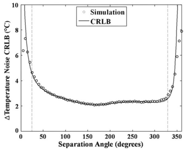
Simulation temperature noise values from NLM-Temp plotted along with the CRLB temperature noise calculations, both using the same input values. These are shown from separation angle to 1° − 360° and a starting angle of 180°. The regions between the dashed lines and the edges are regions of estimation bias where the mean of the simulation deviated from the true value (by >1%)

Investigation of the temperature noise CRLB of fat–water signals for various effects

Single-peak versus multi-peak CRLB

The results from the single versus multi-peak comparison showed very little difference between the CRLBs. Overall, the multi-peak model increased the minimum temperature noise CRLB by approximately 5.5% compared to the single-peak model. For all starting and separation angle combinations, the increase in the CRLB was minimal.

Examination of T2* effects

The temperature noise CRLB values as a function of rotation for varying $\mathrm{T}{2}_{\mathrm{f}}^{\ast }$ values and a constant $\mathrm{T}{2}_{\mathrm{w}}^{\ast }=40\mathrm{ms}$ are shown in Fig. 4. The general trend indicates a minimum near rotation = 4. The minimum of the temperature noise CRLB occurs when the TE values of the ESG are approximately equal to the lowest value of $\mathrm{T}{2}_{\mathrm{w}}^{\ast }$ and $\mathrm{T}{2}_{\mathrm{f}}^{\ast }$. This mimics behavior seen in normal PRFS thermometry, where imaging at the T2* value provides a good compromise between obtaining a large temperature-based phase accumulation (to improve temperature change discrimination) and loss of precision due to decreasing SNR at longer echo times [29]. However, trying to adjust the rotation of an ESG to the T2* value seen in each hyperthermia heat treatment would not be feasible. Fortunately, low-temperature noise CRLB values are consistently seen at rotation = 4 for all values of $\mathrm{T}{2}_{\mathrm{f}}^{\ast }$, as seen by the arrow in Fig. 4. While these values may not be the minimum temperature noise CRLB value for the simulations, they form a practical, good choice based on T2* values typically observed in vivo for fat. Thus, choosing a rotation of 4 (approximately 18 ms for typical fat spectra at 1.5T) should provide a consistently low-temperature noise CRLB regardless of T2* values. Note that with a $\mathrm{T}{2}_{\mathrm{f}}^{\ast }$ less than $\mathrm{T}{2}_{\mathrm{w}}^{\ast }$, we observed sizeable, increasing fluctuations in the temperature noise CRLB with rotation number, possibly due to the presence of multiple peaks.

Fig. 4.

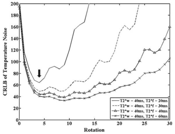
Temperature noise CRLB across several rotations for a constant $\mathrm{T}{2}_{\mathrm{w}}^{°}$ and $\mathrm{T}{2}_{\mathrm{f}}^{\ast }$. Performed with SNR 1, A_water/A_fat = 1, ΔT = 10°C, and ψ = −12.5 Hz. Note the minimum noise near rotation = 4, as noted by the arrow in the figure

Effect of starting TE and TE spacing

The temperature noise CRLB values are shown as 2D intensity images in Fig. 5 for 3-echo, 5-echo, and 7-echo ESGs with rotation = 4, starting and separation angles from 1° − 360°, stepping by 1°. These images will be referred to as temperature noise CRLB maps. The white regions in Fig. 5 are regions outside of the range of the intensity display, since a narrow range was needed to emphasize the structure of the temperature noise CRLB maps in regions of low noise. The minimum temperature noise CRLB of the non-uniform echo spacing was only 2.4% smaller than the minimum temperature noise of the uniform echo spacing. Thus, our optimization analysis performed in this paper should apply to all sampling possibilities.

The temperature noise maps display several interesting features. First, ESGs with very low or very high separation angle typically have a high CRLB, which most likely correlates with the fact that each echo in those ESGs differs little in phase. Also, each temperature noise CRLB map tends to have a several minima, with the number of minima equal to N (the number of echoes). Even with these minima, there is still a wide range of low-temperature noise values typically centered on the separation angle of 180°. However, the width of this region extends when N increases.

Effect of fat–water frequency difference

In this experiment, the fat–water frequency separation was adjusted from 202–222 Hz, the temperature noise CRLB values shifted diagonally across the map with changes in the fat–water frequency difference. In fact, from φ_fw1 = 202 Hz to 222 Hz, minima became maxima and vice versa. These result in changes in the temperature noise from 40° to 70°C, or 0.4 to 0.7°C at SNR = 100. These changes between different fat–water frequency values can be particularly problematic since the frequency values can vary between different regions of the body [26].

Effect of fat/water signal ratio

The most obvious effect seen from changes in the f/w signal ratio was the similar changes in the temperature noise CRLB values for all starting angle and separation angle pairs. These changes were investigated in detail for the starting angle = 150° and separation angle = 150° pair, with results shown in Fig. 6. The temperature noise CRLB is centered around its minimum at A_water/A_fat = 1, or 50:50 water/fat. However, large increases are not seen until the fat percentage gets above 80% or below 20%. This demonstrates that the CRLB is dependent on both the water and fat signals being present in reasonable amounts. Most likely this is due to the fact that the water signal and fat signal must be present in sufficient quantity for accurate measurement of the temperature change and the B₀ field offset, respectively.

Fig. 6.

Temperature noise CRLB for starting angle = 150°, separation angle = 150°, and rotation = 4 for a varying fat signal %. (left) Behavior at the low and high % fat (right) zoomed in y axis to show the behavior at medium % fat. Performed with SNR = 1, ΔT = 10°C, and ψ = −12.5 Hz

Combined effect of fat–water frequency difference, fat/water signal ratio, and temperature change

Because the previously mentioned variables (fat–water frequency difference, ΔT, and f/w signal ratio) have significant individual effects on the temperature noise CRLB, we constructed a multifactorial calculation to allow us to select a starting and separation angle pair that would produce minimal changes in the temperature noise across many situations. The standard deviation of the combined CRLB temperature values from varying ΔT, f/w signal ratio, and fat–water frequency separation are shown for 3-echo, 5-echo, and 7-echo ESGs in Fig. 7. These maps show that the region with the least combined noise occurs near a starting angle = 215° and a separation angle = 240° for three echoes (TEs = 20.71, 23.71, and 26.71 ms), starting angle = 150° and seperation angle = 74° for five echoes (TEs = 19.89, 20.82, 21.75, 22.67, 23.60 ms), and starting angle = 135° and separation angle = 53° for seven echoes (TEs = 19.71, 20.37, 21.03, 21.70, 22 =.36, 23.02, 23.69 ms).

Fig. 7.

Multifactorial simulation showing the standard deviation of the temperature noise CRLB as ΔT, f/w signal ratio, and fat–water frequency separation were varied are shown for a 3-echo, b 5-echo, and c 7-echo ESGs. φ_fw1 was varied from −190 to −240 Hz by 1 Hz, the fat–water signal ratio was varied from 10% fat to 90% fat, in increments of 10% and the temperature change was varied from 0°C − 15°C in 5°C increments. The gray scale bar is in units of °C. Performed with SNR = 1, A_water/A_fat = 1, ΔT = 10°C, and ψ = −12.5 Hz

Effect of number of echoes used

Lastly, the behavior of the temperature noise when the number of echoes was adjusted was examined. The minimum CRLB error with the number of echoes ranging of 3 to 15 echoes is shown in Fig. 8. As might be expected, we found that the minimum temperature noise CRLB follows a power function on the order of x^0.5, as shown by the fit in Fig. 8 (70.03×^0.49 with R² = 1.0). Thus, the improvements in the CRLB tend to closely mimic improvements from SNR due to signal averaging. However, these beneficial effects are for extra echoes past rotation = 4. Adding TE values that are below rotation = 4 (rotations 0, 1, and 2) results in much smaller improvements to the temperature noise CRLB than the improvements seen in Fig. 8. Thus, it is best to acquire as many of the echoes as possible around rotation = 4 to provide the maximum theoretical benefit to the temperature noise CRLB.

Fig. 8.

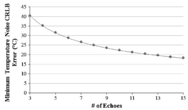
CRLB minimum temperature noise for number of echoes, N, varying from 3 to 15. A power-law fit line is shown along with the equation obtained from the fit

Optimal sampling parameters

With all the previous simulations to determine the effect of certain parameters on the temperature noise of multi-echo thermometry, some conclusions can be made on the optimal sampling parameters, keeping in mind that different trade-offs may be dictated by special circumstances. Since diminishing returns occur with increasing the number of echoes, we recommend seven echoes at rotation =4, and starting angle = 135° and separation angle = 53° (TEs = 19.71, 20.37, 21.03, 21.70, 22.36, 23.02, 23.69ms) for low, stable temperature noise without increasing TR significantly.

Heating and temperature noise measurements in fat/water phantoms

Phantom heating experiment

An MR image of the 50:50 phantom inside the RF applicator before heating is shown in Fig. 9. MR temperature measurements are shown for the 50:50 phantom for the 3- and 5-echo ESG measurements along with fluoroptic probe measurements in Fig. 10. The average root mean-squared deviation of all time points was calculated for each catheter location, with the average deviation across all catheters being 0.227°C for the 3-echo ESG and 0.195°C for the 5-echo ESG. The standard deviation of the temperature measurement was calculated for the nine time points before heat was activated was 0.234°C for the 3-echo ESG and 0.171°C for the 5-echo ESG, while the temperature noise CRLB was 0.234°C for the 3-echo ESG and 0.168°C for the 5-echo ESG. These results show that the NLM-Temp method can measure temperature accurately and that the temperature noise matches the CRLB estimate in experimental situations.

Fig. 9.

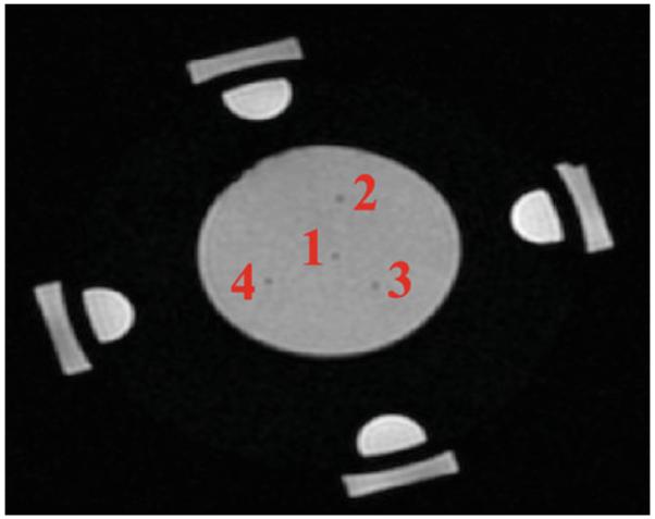
Experimental setup of the phantom heating experiment in the RF applicator. The catheters are labeled to correspond to the labels in Fig. 10

Fig. 10.

Temperature measurement results from the phantom heating experiment with a 3-echo ESG, and b 5-echo ESG. The solid lines are temperatures from the fluoroptic temperature probes while the markers correspond to the MR temperature. Each fluoroptic temperature and MR temperature are marked by numbers that correspond to the locations in Fig. 9

Phantom temperature noise measurement

The measured temperature noise of the 3-echo, 5-echo, and 7-echo ESGs plotted against the expected CRLB standard deviations are shown for the 50:50 phantom in Fig. 11. Our experimental measurements using fat–water phantom experiments show excellent agreement to the temperature noise CRLB calculations presented in this paper. Due to the large number of samples acquired (5,000), the error bars of the measurements are too small to be seen on the plots (on the order of 0.001°C). On average, the measured values vary from the temperature noise CRLB by less than 10.06, 7.40, and 8.78% for 3-echo, 5-echo, and 7-echo, respectively.

Fig. 11.

Phantom results of measured temperature noise and CRLB temperature noise for 3-echo, 5-echo, and 7-echo ESGs. The black line is the CRLB temperature noise predictions plotted against themselves, while the markers are the measured noise values plotted against the CRLB temperature noise predictions

The 50:50 phantom results were closest to the CRLB predictions, while the 70:30 phantom results were less parallel to and farthest from the CRLB predictions. Most of the discrepancies seen in the both the phantom heating and temperature noise experiments are most likely due to limitations in our model and in our measurement of the fat peaks.

While the plots in Fig. 11 may lack data points across the entire range of measurement, we found it more important to sample in many different locations in the lower noise range, where the differences between noise values at different ESGSs was more complex and where we needed to confirm that the noise relationship with the sampling was valid. Additionally, the regions lacking data points were often regions in which the NLM-Temp estimation is biased. Thus, we chose to show data only from the unbiased regions.

Possible limitations in temperature and temperature noise measurements

First, our model assumes that all the fat peaks had the same $\mathrm{T}{2}_{\mathrm{f}}^{\ast }$, which is typically not the case. Also, the model did not include J-coupling, which is present in varying amounts in all the fat peaks. The coupling was ignored since modeling J-coupling can be very complex, especially when peaks are combined together. However, the effect of not including J-coupling was probably a smaller effect since several of the peaks with a large amount of coupling were combined, while the frequency difference between the peaks was much larger than the J-coupling constant of fat (approximately 7 Hz).

Additional limitations in our phantom measurements could have been caused by the estimation of the fat peaks using PRESS. First, the relative ratios of each peak were determined from PRESS spectra taken at TE = 30 ms. However, the measurements used for the fitting ranged from 7.8 to 33 ms. Thus, the ratios calculated from the PRESS spectra probably did not match well at some of the earlier TE times used in the fitting. In addition, our assumption of the same $\mathrm{T}{2}_{\mathrm{f}}^{\ast }$ for all fat peaks may have caused some of the discrepancies. Lastly, as seen in previous studies, the J-coupling present in all of the fat peaks can create significant error in the areas under each peak (and thus the relative ratios) when using PRESS [30].

Temperature changes could have potentially caused errors. First, increases in temperature would cause changes in T1 relaxation, affecting the magnitude of the fat and water signals. However, since our fitting algorithm fits for A_water and A_fat, these changes should be accounted for. Additionally, for the temperature noise experiments, small variations in temperature across the phantom could have increased the measured standard deviation and produced errors. However, the fiber-optic temperature probe data indicates that temperature change was not a large source of error in this experiment. The data set with the largest temperature change over the experiment was the 50:50 3-echo experiment, which had an average temperature change of approximately 0.041°C over the six ESG measurements. The rest of the other experiments had much smaller temperature changes.

Conclusion

In this work, we have extended past temperature noise CRLB formulations for multi-echo fat–water imaging to include temperature change measurement, T2* effects, and multiple fat peaks. This CRLB formulation was then verified with Monte Carlo simulations using a nonlinear fitting algorithm that directly fit for temperature change and B₀ offset from multiple echoes. Many variables of the CRLB calculations were altered to assess their effect on the CRLB, providing a comprehensive analysis of the effects of scan parameters on temperature noise. These variables included the number of TE values, the choice of TE values, T2*, fat–water frequency difference, B₀ offset, temperature change, and fat/water signal ratio. Optimal TE values were found that reduce the standard deviation of the temperature noise when all of the variables were adjusted. Finally, three fat–water phantoms of varying fat/water ratios were imaged with ESGs of 3, 5, and 7 echoes. The resulting measured temperature noise was then compared to calculated CRLB values and were found to be within 10% of each other. This is the first time, to our knowledge, that CRLB values have been experimentally verified extensively in fat–water phantoms.

Overall, the optimization performed in this study can be used to improve the sampling of multi-echo MR thermometry techniques. Increasing the understanding of sampling for multi-echo thermometry will improve the accuracy of the technique and make it a more viable option for MR thermometry. In the breast or abdomen where respiratory and cardiac motions affect the local magnetic field, the multi-echo approach can provide benefits by allowing the local field to be measured. Even if suitable fat–water tissue does not cover the whole region, it is likely that the field changes can be extended using low-order spatial interpolation anchored by field change measures based on multi-echo estimates.

Appendix

When put in matrix form, the signal from Eq. 1 becomes:

$$s\left(k\right)=C(A_{\text{water}},A_{\text{fat}},\psi ,\Delta T)\rho +∊$$

where

$$C=\left[\begin{array}{cccc}\hfill C_{11}\hfill & \hfill C_{12}\hfill & \hfill C_{13}\hfill & \hfill C_{14}\hfill \\ \hfill C_{21}\hfill & \hfill C_{22}\hfill & \hfill C_{23}\hfill & \hfill C_{24}\hfill \\ \hfill ⋮\hfill & \hfill ⋮\hfill & \hfill ⋮\hfill & \hfill ⋮\hfill \\ \hfill C_{N1}\hfill & \hfill C_{N2}\hfill & \hfill C_{N3}\hfill & \hfill C_{N4}\hfill \end{array}\right]$$

For i = all odd numbers and j = 2, 3, 4,

$$\begin{array}{cc}\hfill & C_{i1}=e^{-\frac{{\mathrm{TE}}_i}{T{2}_w^{\ast }}}\cos \left(2\pi \mathrm{TE}\right(\alpha f_0\Delta \mathrm{T}+\psi \left)\right),\hfill \\ \hfill & C_{ij}=e^{-\frac{{\mathrm{TE}}_i}{T{2}_f^{\ast }}}{\beta }_j\cos \left(2\pi {\mathrm{TE}}_i\left(\Delta f_{fwi}+\psi \right)\right)\hfill \end{array}$$

For i = all even numbers and j = 2, 3, 4,

$$\begin{array}{cc}\hfill & C_{i1}=e^{-\frac{\mathrm{TEi}}{T{2}_w^{\ast }}}\sin \left(2\pi \mathrm{TE}\right(\alpha f_0\Delta \mathrm{T}+\psi \left)\right),\hfill \\ \hfill & C_{ij}=e^{-\frac{{\mathrm{TE}}_i}{T{2}_f^{\ast }}}{\beta }_j\sin \left(2\pi {\mathrm{TE}}_i\left(\Delta f_{fwi}+\psi \right)\right)\hfill \\ \hfill & \rho =\left[\begin{array}{c}\hfill A_{\text{water}}\hfill \\ \hfill A_{\text{fat}}\hfill \end{array}\right]s\left(k\right)=\left[\begin{array}{c}\hfill S_1^R\hfill \\ \hfill S_1^I\hfill \\ \hfill ⋮\hfill \\ \hfill S_N^R\hfill \\ \hfill S_N^I\hfill \end{array}\right]\epsilon =\left[\begin{array}{c}\hfill {\epsilon }_1^R\hfill \\ \hfill {\epsilon }_i^I\hfill \\ \hfill ⋮\hfill \\ \hfill {\epsilon }_N^R\hfill \\ \hfill {\epsilon }_N^I\hfill \end{array}\right]\hfill \end{array}$$

where N is the total number of echo times acquired.

The matrix representation was used to find the Fisher Information Matrix (FIM) using the methods described by Pineda [23]. Our model consisted of four unknowns, A_water, A_fat, ψ, and ΔT. Unbiased estimates of these unknowns were arranged in the matrix, ʋ, which is shown below:

$$v=\left[{\widehat{A}}_{\text{water}}{\widehat{A}}_{\text{fat}}\widehat{\Psi }\Delta \widehat{\mathrm{T}}\right]$$

Using these variables resulted in a 4 × 4 FIM, which was calculated using the following equations that are the same as the ones calculated by Pineda.

$$\begin{array}{cc}\hfill & F(k=1,2,l=1,2)=\frac{1}{{\sigma }_{\epsilon }^2}=\frac{1}{{\sigma }_{\epsilon }^2}{\left[C^{t}C\right]}_{kl}\hfill \\ \hfill & F(k=1,2,l=3,4)=\frac{1}{{\sigma }_{\epsilon }^2}=\frac{1}{{\sigma }_{\epsilon }^2}{\left[C^t\frac{\epsilon C}{\epsilon v_l}\rho \right]}_k\hfill \\ \hfill & F(k=3,4,l=3,4)=\frac{1}{{\sigma }_{\epsilon }^2}{\rho }^t\frac{\partial C^t}{\partial v_k}\frac{\partial C^t}{\partial v_l}\rho \hfill \end{array}$$

The derivations of these equations can be found in Pineda et al [23].

References

- 1.Carter DL, MacFall JR, Clegg ST, Wan X, Prescott DM, Charles HC, Samulski TV. Magnetic resonance thermometry during hyperthermia for human high-grade sarcoma. Int J Radiat Oncol Biol Phys. 1998;40(4):815–822. doi: 10.1016/s0360-3016(97)00855-9. [DOI] [PubMed] [Google Scholar]
- 2.Clegg ST, Das SK, Zhang Y, Macfall J, Fullar E, Samulski TV. Verification of a hyperthermia model method using MR thermometry. Int J Hyperth. 1995;11(3):409–424. doi: 10.3109/02656739509022476. [DOI] [PubMed] [Google Scholar]
- 3.Craciunescu OI, Das SK, McCauley RL, MacFall JR, Samulski TV. 3D numerical reconstruction of the hyperthermia induced temperature distribution in human sarcomas using DE-MRI measured tissue perfusion: validation against non-invasive MR temperature measurements. Int J Hyperth. 2001;17(3):221–239. doi: 10.1080/02656730110041149. [DOI] [PubMed] [Google Scholar]
- 4.Craciunescu OI, Raaymakers BW, Kotte AN, Das SK, Samulski TV, Lagendijk JJ. Discretizing large traceable vessels and using DE-MRI perfusion maps yields numerical temperature contours that match the MR noninvasive measurements. Med Phys. 2001;28(11):2289–2296. doi: 10.1118/1.1408619. [DOI] [PubMed] [Google Scholar]
- 5.Craciunescu OI, Samulski TV, MacFall JR, Clegg ST. Perturbations in hyperthermia temperature distributions associated with counter-current flow: numerical simulations and empirical verification. IEEE Trans Biomed Eng. 2000;47(4):435–443. doi: 10.1109/10.828143. [DOI] [PubMed] [Google Scholar]
- 6.MacFall JR, Prescott DM, Charles HC, Samulski TV. 1H MRI phase thermometry in vivo in canine brain, muscle, and tumor tissue. Med Phys. 1996;23(10):1775–1782. doi: 10.1118/1.597760. [DOI] [PubMed] [Google Scholar]
- 7.Samulski TV, Clegg ST, Das S, MacFall J, Prescott DM. Application of new technology in clinical hyperthermia. Int J Hyperth. 1994;10(3):389–394. doi: 10.3109/02656739409010283. [DOI] [PubMed] [Google Scholar]
- 8.Peters RD, Hinks RS, Henkelman RM. Ex vivo tissue-type independence in proton-resonance frequency shift MR thermometry. Magn Reson Med. 1998;40(3):454–459. doi: 10.1002/mrm.1910400316. [DOI] [PubMed] [Google Scholar]
- 9.de Zwart JA, Vimeux FC, Delalande C, Canioni P, Moonen CT. Fast lipid-suppressed MR temperature mapping with echo-shifted gradient-echo imaging and spectral-spatial excitation. Magn Reson Med. 1999;42(1):53–59. doi: 10.1002/(sici)1522-2594(199907)42:1<53::aid-mrm9>3.0.co;2-s. [DOI] [PubMed] [Google Scholar]
- 10.Weidensteiner C, Quesson B, Caire-Gana B, Kerioui N, Rullier A, Trillaud H, Moonen CT. Real-time MR temperature mapping of rabbit liver in vivo during thermal ablation. Magn Reson Med. 2003;50(2):322–330. doi: 10.1002/mrm.10521. [DOI] [PubMed] [Google Scholar]
- 11.Kuroda K, Oshio K, Chung AH, Hynynen K, Jolesz FA. Temperature mapping using the water proton chemical shift: a chemical shift selective phase mapping method. Magn Reson Med. 1997;38(5):845–851. doi: 10.1002/mrm.1910380523. [DOI] [PubMed] [Google Scholar]
- 12.Ishihara Y, Calderon A, Watanabe H, Okamoto K, Suzuki Y, Kuroda K. A precise and fast temperature mapping using water proton chemical shift. Magn Reson Med. 1995;34(6):814–823. doi: 10.1002/mrm.1910340606. [DOI] [PubMed] [Google Scholar]
- 13.Corbett RJ, Laptook AR, Tollefsbol G, Kim B. Validation of a noninvasive method to measure brain temperature in vivo using 1H NMR spectroscopy. J Neurochem. 1995;64(3):1224–1230. doi: 10.1046/j.1471-4159.1995.64031224.x. [DOI] [PubMed] [Google Scholar]
- 14.Corbett RJ, Purdy PD, Laptook AR, Chaney C, Garcia D. Noninvasive measurement of brain temperature after stroke. AJNR Am J Neuroradiol. 1999;20(10):1851–1857. [PMC free article] [PubMed] [Google Scholar]
- 15.Soher BJ, Wyatt C, Reeder SB, MacFall JR. Noninvasive temperature mapping with MRI using chemical shift water-fat separation. Magn Reson Med. 2010;63(5):1238–1246. doi: 10.1002/mrm.22310. [DOI] [PMC free article] [PubMed] [Google Scholar]
- 16.Sprinkhuizen SM, Bakker CJ, Bartels LW. Absolute MR thermometry using time-domain analysis of multi-gradient-echo magnitude images. Magn Reson Med. 2010;64(1):239–248. doi: 10.1002/mrm.22429. [DOI] [PubMed] [Google Scholar]
- 17.Li C, Pan X, Ying K, Zhang Q, An J, Weng D, Qin W, Li K. An internal reference model-based PRF temperature mapping method with Cramer–Rao lower bound noise performance analysis. Magn Reson Med. 2009;62(5):1251–1260. doi: 10.1002/mrm.22121. [DOI] [PubMed] [Google Scholar]
- 18.Scott BR, Zhifei W, Huanzhou Y, Angel RP, Garry EG, Michael M, Norbert JP. Multicoil Dixon chemical species separation with an iterative least-squares estimation method. Magn Reson Med. 2004;51(1):35–45. doi: 10.1002/mrm.10675. [DOI] [PubMed] [Google Scholar]
- 19.Johnson KM, Chebrolu V, Reeder B Scott. Absolute temperature imaging with non-linear fat/water signal fitting. Proceedings of the international society of magnetic resonance in medicine; Toronto, ON. 2008. [Google Scholar]
- 20.Wyatt C, Soher BJ, MacFall JR. Correction of breathing-induced errors in magnetic resonance thermometry of hyperthermia using multiecho field fitting techniques. Med Phys. 2010;37(12):6300. doi: 10.1118/1.3515462. [DOI] [PMC free article] [PubMed] [Google Scholar]
- 21.Van-Trees H. Detection, estimation and modulation theory: part I. Wiley; New York: 1968. [Google Scholar]
- 22.Barrett H, Myers KJ. Foundations of image science. Wiley; New York: 2004. [Google Scholar]
- 23.Pineda AR, Reeder SB, Wen Z, Pelc NJ. Cramer–Rao bounds for three-point decomposition of water and fat. Magn Reson Med. 2005;54(3):625–635. doi: 10.1002/mrm.20623. [DOI] [PubMed] [Google Scholar]
- 24.Yu H, Shimakawa A, McKenzie CA, Brodsky E, Brittain JH, Reeder SB. Multiecho water-fat separation and simultaneous R2* estimation with multifrequency fat spectrum modeling. Magn Reson Med. 2008;60(5):1122–1134. doi: 10.1002/mrm.21737. [DOI] [PMC free article] [PubMed] [Google Scholar]
- 25.Richard K, Michael AW, Kenneth SL, Kuya T, Huanzhou Y, Ann S, Jean HB, Scott BR. Improved fat suppression using multipeak reconstruction for IDEAL chemical shift fat-water separation: application with fast spin echo imaging. J Magn Reson Im. 2009;29(2):436–442. doi: 10.1002/jmri.21664. [DOI] [PMC free article] [PubMed] [Google Scholar]
- 26.McDannold N, Barnes AS, Rybicki FJ, Oshio K, Chen NK, Hynynen K, Mulkern RV. Temperature mapping considerations in the breast with line scan echo planar spectroscopic imaging. Magn Reson Med. 2007;58(6):1117–1123. doi: 10.1002/mrm.21322. [DOI] [PubMed] [Google Scholar]
- 27.Madsen EL, Hobson MA, Frank GR, Shi H, Jiang J, Hall TJ, Varghese T, Doyley MM, Weaver JB. Anthropomorphic breast phantoms for testing elastography systems. Ultrasound Med Biol. 2006;32(6):857–874. doi: 10.1016/j.ultrasmedbio.2006.02.1428. [DOI] [PMC free article] [PubMed] [Google Scholar]
- 28.Soher BJ, van Zijl PC, Duyn JH, Barker PB. Quantitative proton MR spectroscopic imaging of the human brain. Magn Reson Med. 1996;35(3):356–363. doi: 10.1002/mrm.1910350313. [DOI] [PubMed] [Google Scholar]
- 29.de Zwart JA, van Gelderen P, Kelly DJ, Moonen CT. Fast magnetic-resonance temperature imaging. J Magn Reson B. 1996;112(1):86–90. doi: 10.1006/jmrb.1996.0115. [DOI] [PubMed] [Google Scholar]
- 30.Hamilton G, Middleton MS, Bydder M, Yokoo T, Schwimmer JB, Kono Y, Patton HM, Lavine JE, Sirlin CB. Effect of PRESS and STEAM sequences on magnetic resonance spectroscopic liver fat quantification. J Magn Reson Imaging. 2009;30(1):145–152. doi: 10.1002/jmri.21809. [DOI] [PMC free article] [PubMed] [Google Scholar]