

Abstract
MR scans are sensitive to motion effects due to the scan duration. To properly suppress artifacts from non-rigid body motion, complex models with elements such as translation, rotation, shear, and scaling have been incorporated into the reconstruction pipeline. However, these techniques are computationally intensive and difficult to implement for online reconstruction. On a sufficiently small spatial scale, the different types of motion can be well-approximated as simple linear translations. This formulation allows for a practical autofocusing algorithm that locally minimizes a given motion metric – more specifically, the proposed localized gradient-entropy metric. To reduce the vast search space for an optimal solution, possible motion paths are limited to the motion measured from multi-channel navigator data. The novel navigation strategy is based on the so-called “Butterfly” navigators which are modifications to the spin-warp sequence that provide intrinsic translational motion information with negligible overhead. With a 32-channel abdominal coil, sufficient number of motion measurements were found to approximate possible linear motion paths for every image voxel. The correction scheme was applied to free-breathing abdominal patient studies. In these scans, a reduction in artifacts from complex, non-rigid motion was observed.
Keywords: motion correction, autofocus, non-rigid motion, Butterfly, abdominal
Introduction
Motion is a major source of artifacts for Magnetic Resonance (MR) studies. A typical sequence prescribed on the scanner takes anywhere from a couple seconds to a number of minutes. As a result, the scan is sensitive to motion. Motion can come from any number of sources including respiration, cardiac motion, blood flow, and even unintentional patient movement. The effects have been long studied and have been typically observed as ghosting, intensity changes, and blurring (1).
Motion artifacts can be reduced significantly with breath-held scans (2). However, this can be difficult to implement in practice, especially when imaging pediatric patients or when scan time is greater than 20-30 seconds. Costly sedation or anesthesia procedures are required for pediatric patients who are unable to achieve a sufficiently long breath-hold. Data acquisition can also be gated using measurements from respiratory bellows (3) or electrocardiography (4). With these methods, scan duration is increased and the data is still sensitive to bulk motion. Countless motion prevention and correction techniques have been developed. These algorithms are applied during the scan or in the reconstruction. For more flexibility, we will focus on free-breathing studies and on suppressing motion retrospectively in the reconstruction.
In order to correct for non-rigid motion, an accurate motion model must be used. Bulk translational (5) and rotational (6) motion estimation are sufficient for rigid-body scans, but they do not capture the complexity of more general motion. A generalized matrix model (7) has been demonstrated to be effective in parallel reconstruction for non-rigid motion correction (8, 9). Additionally, a sophisticated model can be derived using image registration (10, 11). These models are quite accurate; however, the complexity of these models also increase the complexity of the algorithms. For non-rigid motion, it has been recently proposed to perform affine operators locally (12). We propose an even simpler model: given a sufficiently small region of interest, non-rigid motion can be approximated by localized linear translations.
For this model to be effective, accurate motion measurements must be obtained. Many techniques have been developed to acquire this information. These techniques include using external monitors (13, 14) and using navigator data acquisitions (5, 15). The navigator data can be obtained as a separate acquisition. It can also be built into the k-space trajectory (16-20). Motion information can also be extracted directly from the data (21-23) or from the DC signal (24). For our application of Cartesian imaging, we implement a technique based on the so-called “Butterfly” sequence (19, 20). Butterfly is a modification of the spin-warp sequence in which the pre-winder gradients for phase-encodes are modified slightly to traverse the same trajectory at the beginning of each data acquisition. This makes it possible to obtain translational motion estimates with high temporalresolution. The advantage of Butterfly is that it has negligible overhead for the imaging sequence and is particularly attractive for fast gradient-echo sequences. Navigator data can be improved using redundant data from a multi-channel coil array to help extract more accurate information (25, 26). Recently, there has been interest in exploiting the different sensitivities of receiving coils for more localized measurements (27). We investigate the concept of using multi-channels further using the Butterfly trajectory.
Measuring local motion using a coil array is not sufficient for correction using simple translations, because data from each coil still exhibit a degree of affine motion (12). Therefore, we turn to the concept of autofocusing – the suppression of motion artifacts through the minimization of a metric (28). Because of the countless possible motion paths, autofocusing techniques have been limited to global rigid-body motion (29-33). We hypothesize that with a dense enough receiving coil array, the motion measurements provide a good basis of possible motion exhibited by each image voxel. This limits the search space tremendously. Using the model of simple localized translations, we propose to implement a spatially-dependent autofocusing scheme to suppress non-rigid motion artifacts.
We present the complete procedure – from how the motion measurements are acquired to the details of the autofocusing algorithm. The stability and accuracy of the motion measurement technique is validated with phantom studies. With motion measured in abdominal studies, the localized autofocusing scheme is demonstrated to reduce non-rigid motion artifacts.
Methods
Localized autofocusing in MR applications has had some success in the area of off-resonance correction (34, 35). We apply a similar approach to motion effects. By incorporating a localized motion-artifact metric, it is hypothesized that non-rigid motion can be approximated and corrected using local image translations. A key problem in making this idea clinically possible is that the search space for all possible motion paths is vast and the computational load can quickly become impractical. Therefore, we address this issue and propose a feasible solution.
Motion Measurement Using Butterfly
To confine our search space, the motion is measured during data acquisition. The multi-channel coil array is used as a means of measuring spatially-localized navigator data by exploiting the different local sensitivity maps of each channel. This setup can produce more accurate local motion information. This differs from conventional motion measurement where only one bulk measurement is made for the entire imaged body (5, 15-18, 25). The result is dominated by areas of the largest signal. From a coil array of M coils, M different motion measurements can be estimated. These estimates provide a good search space for the autofocusing algorithm and limit the search space significantly. This set can be expanded and adjusted, but for the scope of this paper, we confine ourselves to the M measurements. As seen in the results, this limitation still provides noticeable improvements.
Navigator Data Acquisition
In order to obtain the M different motion paths, a variant of the Butterfly trajectory (19, 20) is implemented for Cartesian imaging. In general, the Butterfly trajectory acquires navigator data during the pre-winders (and optionally, the re-winders). This feature only requires a negligible time penalty; this approach can be generalized to any sequence that uses pre-winders. It is especially useful for fast acquisitions such as real-time imaging, fast steady-state gradient-echo imaging, and fMRI studies. By using this trajectory, navigator data can be obtained for each coil without significant effects on the sequence used. Additionally, there is no need to make sure the measurements are aligned properly with the acquired data – a concern when using external monitors (13).
In a traditional spin-warp sequence, the pre-winder phase-encode gradients are scaled such that a new k-space line is acquired for every repetition time (TR). In the original Butterfly trajectory as described in Refs. (19, 20), these phase-encode gradients are modified slightly such that in the beginning of the pre-winder, the same gradient is applied for every TR. The rest of the pre-winder is designed to achieve the total gradient area necessary to acquire each k-space line. This modification allows the traversal through k-space along the same diagonal trajectory for every TR. Data collected during that time can serve as navigation information. Figure 1a illustrates the trajectory. Note that the resulting trajectory shape resembles a butterfly wing – hence its name.
FIG. 1.

Butterfly navigator sequence. a: Two-dimensional Butterfly trajectory – original trajectory (left) and proposed trajectory (right). b: Pulse sequence timing diagram for an example three-dimensional Butterfly trajectory. c: Phase/slice encoding effect on the motion measurement – sequential phase/slice encode ordering (left), zigzag phase/slice encode ordering (right), and resulting motion measurements dx for a motionless scan (middle). In (a), the phase-encode ordering is numbered on the left. For the modified Butterfly trajectory, this is just an example of a possible ordering.
This trajectory is very effective in estimating translational motion in two-dimensions. However, it has several limitations which become more obvious for three-dimensional studies. The additional encoding direction increases the navigator’s sensitivity to system error such as gradient delays and eddy-currents; the longer scan time increases the amount of error accrued. Also, there is not much flexibility in choosing the phase/slice encode ordering. For the two-dimensional case, the original trajectory acquires navigator data along the upper-left quadrant diagonal and along the lower-left quadrant diagonal in k-space. If we want to interleave the acquisition of the two different diagonals, we must alternate between acquiring a k-space line in the upper quadrant and a k-space line in the lower quadrant.
To address these concerns, the Butterfly navigators are modified to acquire data along each axis. This modification gives us three main advantages. First, only one gradient-coil at a time is used for the navigator acquisition. This method increases robustness to certain system errors such as different timing delays among the imaging gradients. These timing delays result in simple shifts in the navigator acquisition. Second, the computational complexity for extracting the motion estimate is reduced. Lastly, there is added flexibility in the phase/slice encode ordering – making the method practical for applications that use special ordering such as elliptic centric ordering (36). This variant of the Butterfly trajectory costs an additional time penalty – total of ~ 0.5 ms per TR for a navigator readout duration of 0.14 ms (see Appendix A for more details). An example of this modified Butterfly trajectory is shown in Fig. 1a. The pulse-sequence timing diagram is shown in Fig. 1b for a three-dimensional scan.
Other systematic errors such as eddy currents and gradient hysteresis still affect the stability of the navigator data. To reduce these effects, the phase/slice encodes for three-dimensional scans are ordered in a way that the distance traveled in k-space between each phase/slice encode is minimized. Then, the differences in gradient waveforms from TR to TR are minimized to reduce the change in eddy current and gradient hysteresis effects. This allows for better motion estimation when comparing two subsequent navigators. For simplicity, we used a zigzag ordering of the phase/slice encodes and noticed a reduction factor of ~2 in motion measurement fluctuations (Fig. 1c). As long as the distance between each encode is small, a more sophisticated phase/slice encode ordering can be implemented. Interestingly, the observed eddy currents are not due to the Butterfly navigators. When using fast RF-spoiled gradient echo sequences, we noticed that eddy currents from overlapping rewinders and crushers at the end of each TR affect the slab selection for the next TR. This effect is small and is not observed in the imaging. However, it does create phase variations that result in motion estimate fluctuations on the order of ±0.05 mm.
Motion Extraction from Navigator Data
Our assumption is that each coil element has very localized sensitivity. In this case, the motion observed for each coil image is approximated as a linear translation – a linear-phase shift in the frequency domain,
| [1] |
The navigator data are the first L samples of each readout, where index l ∈ [0 … L] enumerates the samples and corresponds to the time of acquisition (within a TR). Index n, on the other hand, corresponds to the TR number. For nth navigator signal sn[l], linear translation d[n] = (dx[n], dy[n], dz[n]) is modeled as a linear-phase modulation applied to the reference navigator signal, s0[l]. Three-element vector k = (kx, ky, kz) represents the k-space location. Signals s0[l] and sn[l] both correspond to k-space location k[l]. For generality, x, y, and z respectively represent the readout, phase-encode, and slice-encode axes. In Eq. [1], motion is assumed to only occur between each data acquisition. This is a reasonable model given a short readout.
When estimating d[n], care must be taken to ensure robustness against signal fluctuations. The modification to the Butterfly acquisition reduces some of the systematic errors. Precautions must also be taken during post-processing. These errors are unavoidable; for example, motion relative to each coil results in changes in the signal intensity (25). Additionally, B0 eddy currents contribute to signal fluctuations. To account for observed errors, Eq. [1] was modified to include bulk magnitude and phase fluctuations. The magnitude and phase fluctuations are represented by a complex scaling factor .
| [2] |
Many methods exist to estimate d[n] in either the image domain or the frequency domain. Image-domain based algorithms (5, 15, 37) require a transformation from the acquired k-space data into the image space. Since the Butterfly navigators are acquired during the ramp of the pre-winder gradients, the data is acquired with linearly increasing spacings along a single-sided k-space spoke. This makes it difficult to perform an accurate non-uniform Fourier transform. A couple of fast frequency-domain based algorithms are also commonly used (38, 39). Unfortunately, these schemes assume a uniform sampling pattern.
To account for C[n] while estimating d[n], we use an iterative Gauss-Newton method to find parameter values that best fit the nonlinear model in the least-squares sense. The parameter values are calculated by first estimating the magnitude-based parameters. Afterward, the phase-based parameters are estimated. More specifically, the magnitude of C[n], cr[n], is first estimated using least-squares.
| [3] |
The reference signal is updated to s′0[l] = cr[n]s0[l]. Then, cφ[n] and d[n] are estimated with another optimization problem.
| [4] |
The Butterfly navigator samples k-space more densely near the origin where the signal is the highest. Also, for these data points, the eddy current effects are stronger, because they are closer in time to the beginning of the TR. Unfortunately, naive fitting through least-squares will put much weight on these potentially corrupted points. Weights incorporated into the algorithm (Eqs. [3] and [4]) counteract these effects.
| [5] |
| [6] |
A summary of the weighted Gauss-Newton algorithm to solve Eq. [6] is shown in Table 1 for a one-dimensional Butterfly navigator in the x-direction. The same algorithm is used for the y and z navigators. Since the different navigators are interleaved, the motion measurement extracted is interpolated to estimate the full motion path, d[n]. This measurement can be filtered to remove any residual high-frequency signal fluctuations.
Table 1.
Iterative Gauss-Newton algorithm used to estimate motion for the one-dimensional Butterfly navigator in the x direction.
| Weighted Gauss-Newton Motion Estimate | ||
|---|---|---|
| Goal: | ||
| Inputs: | kx[l] – x navigator trajectory of length L | |
| s0[l] – reference signal evaluated at kx[l] | ||
| s[l] – navigator signal evaluated at kx[l] | ||
| w[l] – weights | ||
| ∊1 – stopping criteria 1 | ||
| ∊2 – stopping criteria 2 | ||
| Outputs: | cφ – bulk phase difference | |
| dx – motion estimate as linear translation | ||
|
| ||
| Algorithm: | cφ = 0, dx = 0, sj [l] = s[l] | Initialization |
| do{ | ||
| Construct r: r[l] = w[l] × (s0[l] − sj[l]) | Weighted residual | |
| Construct a1: a1[l] = w[l] × i2πkx[l]sj[l] | ||
| Construct a2: a2[l] = w[l] × i2πsj [l] | ||
| Using weighted least-squares | ||
| dx = dx + dj, cφ = cφ + cj | Update | |
| sj [l] = s[l]e−i2π(kx[l]dx+cφ) | ||
| }while |dj| > ∊1 and |cj| > ∊2 | ||
In our implementation, two different sets of weights are used and the fitting is performed twice. The first set of weights is designed to avoid phase-wrapping. The second is designed to achieve a more accurate estimate of d[n]. For the purpose of avoiding phase-wraps, first, Eqs. [5] and [6] are solved using magnitude-based weights. For example,
| [7] |
The higher-magnitude data points are associated not only with higher signal but also with the data at the beginning of the navigator with smaller sampling spacing in k-space. Closer spacing helps avoid phase-wraps when estimating the linear phase. The weights in Eq. [7] are used to solve Eqs. [5] and [6] with a high error tolerance for a rough estimate. Afterward, the error tolerance is lowered when a second set of weights are used. These weights emphasize the less-corrupted data points with more motion information in the phase:
| [8] |
Both w1[l] and w2[l] are incorporated into a two-stage weighted Gauss-Newton algorithm to quickly solve for the motion estimate.
Motion Correction
After data acquisition and motion extraction from M channels, we have M motion estimates: d1[n], d2[n], … dM[n]. These measurements provide a good search space in finding the motion at each spatial position in the image for each TR. As a simplification, we approximate non-rigid motion as local linear translations rather than rotation, contraction/expansion, and other complicated transformations. Using this model, it is noted that particular image locations can be focused with a given motion path. Therefore, we apply linear-phase correction to all the acquired k-space data with each of the M motion measurements. After transforming to image space, we use a motion-artifact metric to determine locally which measurement yielded the best linear correction (Fig. 2a).
FIG. 2.

Non-rigid motion correction overview. a: Correction scheme using data from an M-channel coil array. b: Linear translational motion correction 29 using motion measurement d1[n]. c: Localized gradient entropy calculation (Eq. 12).
Reduced Computation with an Optional Coil Compression
To reduce computation, it is possible to perform coil compression prior to the linear-phase correction. Coil compression algorithms combine data from multiple channels into fewer so-called “virtual coils”. Coil compression is allowed as long as multi-channel data from the same phase/slice encode acquired at the same time are combined; they exhibit the same motion. A suitable algorithm is the software coil compression by Huang et al (40). In this work, we use an improved algorithm by Zhang et al (41). The compression is achieved by linearly combining the data from the different coils. Therefore, applying the compression weights followed by the linear motion correction of each virtual coil is equivalent to applying the compression weights after the linear motion correction of each original coil.
Rather than performing M2 corrections (M motion paths on k-space data from M coils), the computation is reduced to MMv corrections (M motion paths on Mv virtual coil data). By compressing data from 32 coils to 6 virtual coils, the computation is effectively reduced by a factor of ~5. Note that coil compression is not performed on the navigator data to maintain the localization from the physical coils.
Linear Correction
After coil compression, the Mv virtual coils are corrected by linear translations based on each of the original M motion measurements. Linear translations are fast to correct because they manifest in k-space data as linear phase. For the nth acquisition, the k-space data is corrected using the measured motion, d[n] = (dx[n], dy[n], dz[n]), with the following equation.
| [9] |
The original nth acquired k-space readout line is represented by sn[l]. This line represents data acquired with a frequency encoding of kx[l], a phase encoding of ky[n], and a slice encoding of kz[n]. Motion is assumed to only occur between each TR, but Eq. [9] can be easily extended to support motion during data acquisition.
The formulation in Eq. [9] is applied to each of the Mv virtual coils using motion measurement d1[n]. Afterward, an inverse Fourier transform is applied to the modified k-space data. The resulting images are combined using any preferred coil-combination algorithms. Sum-of-squares is used here for simplicity. A block diagram summarizing this step is shown in Fig. 2b. This linear correction step is performed for each of the M motion estimates.
Localized Motion Metric
After correcting for different motion measurements, we must determine which correction yielded the best result for a particular location. For an objective evaluation, a localized motion-artifact metric is used. McGee et al reviewed 24 different metrics and recommended the use of gradient entropy as a good metric for motion-artifacts (where “gradient” refers to image intensity gradient, represented as ▽, rather than the MR imaging gradients) (28). This criteria is minimized when “the image consists of uniform brightness separated by sharp edges” which they found to be a good model for normal MR scans. They globally applied this gradient entropy metric H.
| [10a] |
| [10b] |
| [10c] |
The complex pixel value of image I at index (i, j, k) is denoted as Iijk. To make the criteria independent of the scan orientation, total absolute gradient is computed. The value of ▽iIijk, ▽ jIijk, and ▽kIijk can be approximated as one-dimensional differences: Ii+1,jk−Iijk, Ii,j+1,k−Iijk, and Iij,k+1−Iijk respectively.
We modified the gradient entropy metric to be a localized metric by calculating Eq. [10] for a selected area around the pixel of interest.
| [11a] |
| [11b] |
For convenience, the three-dimensional summation operator is resented as . Equation [11] can be re-written in terms of h of Eq. [10c] as
| [12] |
Performing the summation operator in Eq. [12] is equivalent to filtering with a moving-average filter. To make the entropy measure more localized to the center of the window, we use a low-pass Hanning filter. We implement a three-dimensional separable Hanning window with a main-lobe width of b. A block diagram of the local gradient entropy calculation is shown in Fig. 2c.
The value of window-width b influences the resulting correction. Fine motion details are captured by smaller values of b. However, b must be sufficiently large to capture anatomical structure; otherwise, motion artifacts are mistakenly amplified. An isotropic window width is used.
| [13] |
Variables δi, δj, and δk represent the image-pixel resolution. Figure 3 shows the result of applying different filtering widths bc to an example case. In all cases, the result is an improvement over the original uncorrected image. For a favorable balance between correction and amplification of artifacts, bc = 10 cm is used. This corresponds to a full width at half maximum of 5 cm.
FIG. 3.

Comparison of different window widths bc for the localized gradient entropy calculations. The window widths bc = 2 cm, 4 cm, and 6 cm are shown for scale. When bc = 2 cm, the arteries appear sharper; however, the ghosting artifact from the fat wall is introduced. Additionally, noise amplification can be noticed outside the body. With bc = 14 cm, the arteries blur and a faint ghosting artifact appears above the liver; this region cannot be successfully approximated as linear translations. For a nice balance, bc = 10 cm is used for our corrections. This corresponds to a full width at half maximum of 5 cm.
With an appropriate motion metric, we can use autofocusing to locally determine which motion measurement yielded the best result for a select region.
| [14a] |
| [14b] |
The motion estimate number is m. The image corrected using motion measurement dm[n] is denoted by I′[m]. The gradient entropy at pixel (i, j, k) for image I′[m] is represented as Hijk[m]. Image Ĩ is the final corrected image. In Eq. [14a], for every voxel in the image, we chose which motion correction (out of the M possible ones) best minimizes the metric. In Eq. [14b], we chose the voxel value corresponding to that correction as the solution.
Experiment
To test the algorithm, studies were performed on a General Electric MR750 3T scanner (Waukesha, WI). A number of phantom studies were conducted to validate the motion measurements from the Butterfly navigator acquisition using a single-channel quadrature head coil. The stability of the motion measurement was analyzed on a motionless phantom. The accuracy of the measurement was analyzed on a moving phantom. A simple linear translation correction was performed to test the quality of the observation. For this case, the scan table was programmed to move periodically in the superior/inferior direction to induce simple rigid motion.
Abdominal studies were conducted using a custom high-density phased array coil constructed at our institution in collaboration with GE Healthcare – a 32-channel pediatric torso receiver coil (42). When scanning the pediatric patients, a portion of the central k-space data was respiratory triggered and gated. This strategy provided accurate data to estimate a reference navigator for motion extraction and to calibrate weights for coil compression. Remaining data were acquired during free-breathing. For all experiments, the scan was performed in the coronal orientation using a three-dimensional spoiled gradient echo acquisition (SPGR) sequence. Specific scan parameters used for each study are summarized in Table 2. The reconstruction was performed on a Linux system with an Intel Core i7-950 3.07GHz Quad-Core processor, 24 GB of RAM, and a NVIDIA GeForce GTX 470 graphics card. The algorithm was implemented using a combination of Matlab (MathWorks, Natick, MA) and C++/CUDA (NVIDIA, Santa Clara, CA).
Table 2.
Scan parameter summary.
| Phantom Study | Study 1 | Study 2 | |
|---|---|---|---|
| TE/TR: | 3.5 ms / 7.3 ms | 2.1 ms / 5.5 ms | 1.7 ms / 4.8 ms |
| Resolution: | 0.88 × 0.88 × 1.0 mm3 | 0.94 × 0.94 × 3.0 mm3 | 0.94 × 1.2 × 3.0 mm3 |
| FOV: | 28.0 × 22.4 × 18.0 cm3 | 30.0 × 24.0 × 15.6 cm3 | 30.0 × 24.0 × 16.2 cm3 |
| Flip angle: | 15° | 15° | 15° |
| Bandwidth: | 62.5 kHz | 62.5 kHz | 62.5 kHz |
| Navigator per TR: | 0.24 ms | 0.14 ms | 0.11 ms |
| Resp gated k-space: | 0% | 10% | 5% |
| Coil: | 1-ch head | 32-ch ped torso | 32-ch ped torso |
Results
The Butterfly motion measurement procedure was first validated on a rigid phantom to determine our confidence in the measurements for patient scans. The stability of the measurements was verified using a motionless phantom (Fig. 4a). Sub-millimeter fluctuations and drift was observed in the motion path plot. The amplitude of these effects were extremely small – much smaller than conventional scan resolution. The quality of the measurements was verified using a phantom with translational rigid motion (Fig. 4b). With a simple linear correction, the motion artifacts were significantly reduced. Due to gradient nonlinearity and possibly off-resonance effects, some residual artifacts remained. Regardless, image quality was significantly improved and the accuracy of the motion measurement procedure was verified.
FIG. 4.

Phantom study results. a: Motionless scan verified the stability of the motion measurements. b: Rigid body translation validated the accuracy of the measurements and correction. For both (a) and (b), dx = superior/inferior motion, dy = right/left motion, and dz = anterior/posterior motion. In (a), a drift of < 0.25 mm was observed for a span of 170 s; this is negligible compared to actual motion, and could be corrected by polynomial fitting. In (b), the motion was accurately measured as shown in the plot. This measurement successfully corrected for significant motion. Some residual ghosting artifacts remained due to gradient nonlinearity.
A free-breathing three-dimensional abdominal study was analyzed, and the results are shown in Fig. 5. The structure of the estimated paths agreed with what was expected: motion was dominated by periodic respiratory motion and a portion of the path was motionless from respiratory gating. Because the center of k-space was gated and relatively motion free, a majority of the motion artifacts were from corrupted data corresponding to higher spatial-frequencies. This resulted in image blurring as seen in the original three-dimensional volume (Fig. 6).
FIG. 5.

Study 1 motion measurements. a: Resulting translation maps displayed in the sagittal (at −77.6 mm from isocenter) and coronal (at 5.8 mm from isocenter) slices at select time points accurately depicting the respiratory motion. b: Motion measurements acquired, where each color is a motion estimate from a different coil c: Histogram plot of number of pixels that was focused by each motion path – the number of pixels gives an idea of the scan volume that was focused by each measurement. In (c), the motion measurement number corresponds to the coil that observed that motion. Measurement number 0 corresponds to the case of no motion. (a) and (b) accurately depict the respiratory motion. Stationary regions in the lower torso were recognized by the algorithm. As expected, each coil observed a different degree of movement.
FIG. 6.

Study 1 results – an abdominal study performed on a 6-year-old patient using a three-dimensional SPGR sequence. first row: Slice 16, 24, 28, and 32 of the original uncorrected three-dimensional volume. second row: Same slices from the corrected volume. third row: Derived translation maps in the coronal plane. fourth row: Maps of the motion measurement number used to correct each pixel. Measurement number maps demonstrate that the motion measured from one coil can extend beyond where that coil is most sensitive. Additionally, correcting with the nearest and most sensitive coil does not always yield optimal results. Ghosting artifacts were suppressed in slice 16. An increase in sharpness and structure can be seen in the liver vessels in slice 28.
Derived translation maps in the sagittal and coronal orientation are shown in Fig. 5a for select time points. These maps agreed with normal respiratory motion. Bulk motion was noticed going from the inferior to superior direction during inspiration. There was a period of little to no motion, followed by bulk motion from the superior to inferior direction during expiration. Additionally, negligible motion was observed in the lower pelvis area where the patient was relatively motionless. In regions of low SNR and regions with little structure, a small degree of motion was mistakenly predicted by the algorithm. Fortunately, these areas were usually areas of little diagnostic value. As we will discuss later, these problems can be mitigated and potentially avoided.
After performing the correction scheme on this first study, noticeable improvements were observed. In Fig. 6, we recovered some of the resolution that was lost from motion corruption. An increase in sharpness and structure was observed along the tissue planes and blood vessels. Some residual arti-facts remained (slice 16). The uncorrected artifacts may be because our motion measurements were unable to capture the exact motion path at these locations. Expanding the motion measurements to a larger search space should improve the correction quality.
A second study on a smaller subject was performed, and the final results are shown in Fig. 7. Less motion was observed overall compared to the first study. However, improvement in image quality was still observed. Ghosting artifacts were reduced. This ghosting artifact may have been easily confused with arterial wall structure as seen in the original slice 28 and 30. Additionally, better definition of tissue planes and of a lesion was achieved.
FIG. 7.

Study 2 results – an abdominal study of a 2-year-old patient with a renal tumor scanned using a three-dimensional SPGR sequence. top row: Slice 19, 23, 28, and 30 of the original uncorrected three-dimensional volume. bottom row: Same slices from the corrected volume. Ghosting artifacts in slice 19 were suppressed, and the tissue planes were sharpened. In slice 23, a lesion became better defined after correction.
Discussion
Motion Metric
The detail and accuracy of the correction depend strongly on how finely we can calculate the motion-artifact metric. However, if we decrease bc to calculate the localized gradient entropy (Eq. [11]) for a very small region, noise or motion artifacts may potentially be amplified. The algorithm needs some edge information for better performance. There are a number of ways to ensure enough detail in the metric without compromising effectiveness.
One method is to use a small bc (< 5 cm) and a criteria to ensure a smooth translation map. For this formulation, Eq. [14a] can be re-written as
| [15] |
The acquisition number n0 can be selected for the point in the path with the largest amount of motion. Variable λ can be adjusted until the desired results are achieved.
Another way to adjust the motion metric is to expand the localized motion metric. Instead of just calculating the localized gradient entropy for one value of bc, two values of bc can be used: a smaller one to differentiate high detail motion and a larger one to ensure some consistency in neighboring regions. The following formulation can be used as the motion metric Hijk in Eq. [14a].
| [16] |
Entropy is calculated using Eq. [11] with a large value of b , and is calculated with a small value of bc. Scalar α is used to adjust the emphasis on translation map detail or to ensure that some edge information is captured. Example parameters used are bc = 12 cm for , bc = 2 cm for , and α = 0.25.
Motion Measurement
The autofocusing performance also depends on the motion measurements for an appropriate search space. By including a null motion path d0[n] = 0, we allow the algorithm to avoid any corrections if no sufficiently-accurate path exists.
Not all of the M measured motion paths were used in the correction (Fig. 5c). For the unused paths, we may have measured an area with no motion, repeated a measurement of another coil, or used a malfunctioning coil. In any case, this observation hints at the possibility to reduce the search space by discarding extraneous measurements. Also, the M measurements can be expanded to create a larger search space for autofocusing and to allow for a more accurate correction. This space can be further explored by using various linear coil-combinations for more localized sensitivities or by using filtering to reduce the FOV of each coil. By applying these operations to the navigator data, additional motion measurements can potentially be extracted. Reducing or extending this search space is not a simple task and is left for an area of future research.
The motion measurements are used to perform localized corrections. If neighboring regions select extremely different motion paths for correction, unnatural discontinuities may arise. By requiring some spatial consistency in the autofocusing formation (Eqs. [15] and [16]), the problem can be mitigated. However, discontinuities may still arise if there are insufficient and/or inconsistent motion measurements. In our experience, measurements using a 32-channel pediatric coil array sufficiently covered the search space. Additionally, the acquisition of the reference navigator, s0[l], was triggered and gated to ensure that the reference is motion-free and at the same motion state (same time point) for all channels.
More coils with more localized sensitivities can help with the accuracy of the motion estimation. More elements to depict the local motion paths, such as rotational movement, can be measured (43-45) and added to the correction model. The autofocusing scheme can determine the best local correction. We provided a practical framework that was able to show improvement by finding the optimal linear corrections in the given set. The motion model and correction algorithm can easily be extended to include more complex features. However, the amount of additional computation required should be considered.
Butterfly Navigator Data Acquisition
The autofocusing technique is independent of the motion measurement procedure. In this work, the multiple measurements were made possible using the Butterfly trajectory. As mentioned, a concern when using the Butterfly trajectory is its sensitivity to system errors. These errors must be properly dealt with to accurately estimate the non-rigid motion as simple linear translations. The motion-extraction formulation in Eqs. [3], [4], [5], and [6] can be extended to include higher-order errors. For example, if the system and/or application is prone to k-space drift Δk[n] = (Δkx[n], Δky[n], Δkz[n]), this term can be added to Eq. [5].
| [17] |
The notation s0(k[l]-Δk[n]) is the signal interpolated from k-space values of k[l] to (k[l]-Δk[n]). This nonlinear optimization problem can be solved using a weighted Gauss-Newton algorithm. Afterward, the reference signal is updated to s′0[l] = cr[n]s0(k[l]-Δk[n]) before Eq. [6] is computed. For our studies (Fig. 4), accurate and stable measurements were obtained using the model in Eq. [2]. In our experiments, 5 iterations of the Gauss-Newton algorithm on average are needed to estimate the linear translation – fast enough for real-time applications.
Implementation
Correction schemes that take significantly longer than the full MR study are impractical to use for clinical applications. Therefore, significant effort was made to make the algorithm computationally efficient. With three-dimensional coil compression from M coils to Mv virtual coils, the computation was reduced significantly.
Minimizing signal lost, the coil compression linearly combines data from the different coils. This process may amplify motion artifacts which can be reduced with a more sophisticated coil combination scheme as discussed in Ref. (46). The correction can be further improved with more sophisticated steps in the proposed autofocusing scheme. For these extensions, a trade-off between computational cost and amount of improvement must be analyzed.
The bulk of the calculations was for computing each linear motion correction and for computing the resulting motion-artifact metric. These steps were implemented using C++/CUDA to take advantage of the parallel computing power of the graphics processing units. On the GeForce GTX 470 card, the linear motion correction for the k-space data of matrix size 320 × 256 × 52 took an average of 0.27 s for one motion path applied to one coil. The calculation of the localized gradient entropy for the same data size on the same processing unit took an average of 0.57 s. For this study, the total computation time was on the order of (0.27Mv + 0.57)(M + 1) s. The additional +1 was for motion path d0[n] = 0. For M = 32 and Mv = 6, the computation time was 72.3 s. Additional computation time is needed for the other steps of the algorithm including memory transfer and coil combination. The total time was still less than 2 min.
Extension to Other Imaging Techniques
The autofocusing scheme is independent of the scan sequence. For practicality, only the local motion measurements are required. In most cases, the Butterfly trajectory can be used to obtain these measurements with a coil array. For scans that do not use pre-winder gradients, other techniques may be applied, such as acquiring the navigator data in an interleaved TR.
This work can also be combined with the use of prospective motion compensation techniques (47, 48). Overly-corrupt data can be re-acquired as in the diminishing variance algorithm (49, 50). Or, the scan parameters can be adjusted to reflect the motion (13, 47, 51). With its high temporalresolution, the Butterfly trajectory could be used to provide motion information in this context. These prospective methods have difficulty in compensating for non-rigid motion; thus, the use of the autofocusing method is still needed.
Other imaging techniques can be used in conjunction with our correction, but the post-processing for these methods may affect the computational complexity. Algorithms that preserve k-space phase, such as gridding for non-Cartesian imaging (52-54) and field inhomogeneity correction (55-57), can be applied before or after coil compression. However, for algorithms that do not preserve k-space phase, such as Homodyne reconstruction (58), these steps must be applied for each motion measurement before the gradient entropy calculation. As long as the time needed to perform these steps is not significant, the scheme is still practical to apply. For example, for a Homodyne implementation on the same graphics card, it takes an average of 0.31 s to reconstruct the full k-space matrix of 320 × 256 × 52 from a data matrix of 192 × 256 × 52. This adds an extra minute to the total computation time.
The localized coil sensitivities provide for more sophisticated techniques. In our method, all the acquired data is used for correction and reconstruction. The measured motion path can be used to retrospectively reject overly-corrupt acquisitions; these acquisitions can be regenerated through accelerated imaging techniques. These techniques can also be used to shorten the overall scan duration. However, the incorporation of accelerated imaging into the proposed scheme is more cumbersome. Parallel reconstruction techniques, such as SENSE (59) and GRAPPA (60), and compressed sensing (61) make use of the consistency of the k-space data. For parallel imaging, the different coil sensitivity maps allow data to be accurately estimated through interpolation functions. Unfortunately, data is also interpolated from acquisitions corrupted by motion, so the motion corruption may spread. A simple solution is to perform the parallel reconstruction during the coil combination stage in Fig. 2b, so that data consistency can be achieved for the focused spatial regions. However, the computational complexity of these techniques increases the computation time significantly.
Conclusion
By approximating non-rigid motion with local linear translations, motion correction can be practically implemented. Through the use of the proposed localized gradient entropy criteria, the correction can be fine-tuned. The algorithm is made practical by reducing the data size using coil compression and by reducing the search space using motion measurements extracted from a coil array. Based on the motion criteria, the algorithm improves the quality of the final images. Results from abdominal studies confirm these improvements.
Acknowledgments
The authors would like to thank Tao Zhang for help with the three-dimensional coil compression.
This work was supported by NIH training fellowship, NIH grants R01 EB009690 & P41 RR09784, UC Discovery Grant #193037, and GE Healthcare.
Appendix A: Butterfly time penalty
The Butterfly modification to the pre-winders allows navigator data to be acquired for every TR. Additionally, to increase robustness to systematic error, navigator data is acquired along each axis rather than along the k-space diagonals. A time penalty is required to implement this approach. We examine an example phase-encode gradient to determine the maximum amount of additional time is needed to implement the modified Butterfly technique.
The original phase-encode gradient is constructed to be limited by the maximum gradient amplitude, Gmax, as shown in Fig. 8a. Time ta is needed to complete the entire pre-winder. In Fig. 8b, the phase-encode gradient is modified to acquire the navigator data for a duration of tn. The slew rate, Snav, determines the extent of the navigator in k-space.
FIG. 8.
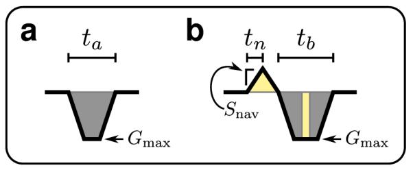
Butterfly time penalty analysis. a: Original phase-encode gradient. b: Butterfly modified phase-encode gradient. For equivalent acquisitions, the total gradient areas in (a) and (b) must be equal. The gradients are designed such that the light-yellow shaded regions have the same areas and the dark-gray shaded regions have the same areas.
In the worst case, the Butterfly navigator is acquired in the opposite k-space direction of the phaseencoding. To compensate for the additional gradient area, the original phase-encode gradient is extended to a duration of tb. For simplicity, we assume the same slew rate is used to ramp down the Butterfly gradient blip. We relate tn, ta, and tb by examining the gradient areas (Fig. 8b).
| [A.1a] |
| [A.1b] |
Since the navigator data is acquired along one gradient axis, an additional time tn is required. This allows the data to be collected before the other gradient axes are turned on. The total time needed for the modified phase-encode gradient is
| [A.2a] |
| [A.2b] |
The time difference tp between the original phase-encode gradient and the Butterfly modified phaseencode gradient is
| [A.3] |
In situations where no phase-encode reaches the gradient limit of Gmax, the maximum gradient amplitude of the phase-encodes can be used in place of Gmax in Eq. [A.3]. The result will be an over-estimate, but it will give a good idea of the actual time penalty. For tn = 0.14 ms, Snav = 200 mT/m/ms, and Gmax = 40 mT/m, the additional time needed is tp = 0.52 ms. This time penalty can be reduced by shortening tn or relaxing Snav. However, with these alterations, the motion information may be compromised.
References
- [1].Wood M, Henkelman R. MR image artifacts from periodic motion. Med Phys. 1985;12:143–151. doi: 10.1118/1.595782. [DOI] [PubMed] [Google Scholar]
- [2].Plathow C, Ley S, Zaporozhan J, Schöbinger M, Gruenig E, Puderbach M, Eichinger M, Meinzer HP, Zuna I, Kauczor HU. Assessment of reproducibility and stability of different breath-hold maneuvres by dynamic MRI: comparison between healthy adults and patients with pulmonary hypertension. Eur Radiol. 2006;16:173–179. doi: 10.1007/s00330-005-2795-9. [DOI] [PubMed] [Google Scholar]
- [3].Ehman RL, McNamara MT, Pallack M, Hricak H, Higgins CB. Magnetic resonance imaging with respiratory gating: techniques and advantages. AJR Am J Roentgenol. 1984;143:1175–1182. doi: 10.2214/ajr.143.6.1175. [DOI] [PubMed] [Google Scholar]
- [4].Lanzer P, Botvinick E, Schiller N, Crooks L, Arakawa M, Kaufman L, Davis P, Herfkens R, Lipton M, Higgins C. Cardiac imaging using gated magnetic resonance. Radiology. 1984;150:121. doi: 10.1148/radiology.150.1.6227934. [DOI] [PubMed] [Google Scholar]
- [5].Ehman R, Felmlee J. Adaptive technique for high-definition MR imaging of moving structures. Radiology. 1989;173:255–263. doi: 10.1148/radiology.173.1.2781017. [DOI] [PubMed] [Google Scholar]
- [6].Atkinson D, Hill DLG. Reconstruction after rotational motion. Magn Reson Med. 2003;49:183–187. doi: 10.1002/mrm.10333. [DOI] [PubMed] [Google Scholar]
- [7].Batchelor PG, Atkinson D, Irarrazaval P, Hill DLG, Hajnal J, Larkman D. Matrix description of general motion correction applied to multishot images. Magn Reson Med. 2005;54:1273–1280. doi: 10.1002/mrm.20656. [DOI] [PubMed] [Google Scholar]
- [8].Odille F, Vuissoz PA, Marie PY, Felblinger J. Generalized reconstruction by inversion of coupled systems (GRICS) applied to free-breathing MRI. Magn Reson Med. 2008;60:146–157. doi: 10.1002/mrm.21623. [DOI] [PubMed] [Google Scholar]
- [9].Odille F, Cîndea N, Mandry D, Pasquier C, Vuissoz PA, Felblinger J. Generalized MRI reconstruction including elastic physiological motion and coil sensitivity encoding. Magn Reson Med. 2008;59:1401–1411. doi: 10.1002/mrm.21520. [DOI] [PubMed] [Google Scholar]
- [10].Buerger C, Schaeffter T, King AP. Hierarchical adaptive local affine registration for fast and robust respiratory motion estimation. Medical Image Analysis. 2011;15:551–564. doi: 10.1016/j.media.2011.02.009. [DOI] [PubMed] [Google Scholar]
- [11].Schmidt JFM, Buehrer M, Boesiger P, Kozerke S. Nonrigid retrospective respiratory motion correction in whole-heart coronary MRA. Magn Reson Med. 2011;66:1541–1549. doi: 10.1002/mrm.22939. [DOI] [PubMed] [Google Scholar]
- [12].Vaillant G, Buerger C, Penney G, Prieto C, Schaeffter T. Multiple-region affine motion correc- tion using localized coil sensitivites; Proceedings of the 19th Annual Meeting of ISMRM; Montreal, Canada. 2011.p. 4605. [Google Scholar]
- [13].Zaitsev M, Dold C, Sakas G, Hennig J, Speck O. Magnetic resonance imaging of freely moving objects: prospective real-time motion correction using an external optical motion tracking system. Neuroimage. 2006;31:1038–1050. doi: 10.1016/j.neuroimage.2006.01.039. [DOI] [PubMed] [Google Scholar]
- [14].Ooi MB, Krueger S, Muraskin J, Thomas WJ, Brown TR. Echo-planar imaging with prospec- tive slice-by-slice motion correction using active markers. Magn Reson Med. 2011;66:73–81. doi: 10.1002/mrm.22780. [DOI] [PMC free article] [PubMed] [Google Scholar]
- [15].Wang Y, Grimm RC, Felmlee JP, Riederer SJ, Ehman RL. Algorithms for extracting motion information from navigator echoes. Magn Reson Med. 1996;36:117–123. doi: 10.1002/mrm.1910360120. [DOI] [PubMed] [Google Scholar]
- [16].Pipe JG. Motion correction with PROPELLER MRI: application to head motion and free- breathing cardiac imaging. Magn Reson Med. 1999;42:963–969. doi: 10.1002/(sici)1522-2594(199911)42:5<963::aid-mrm17>3.0.co;2-l. [DOI] [PubMed] [Google Scholar]
- [17].Liu C, Bammer R, Kim DH, Moseley ME. Self-navigated interleaved spiral (SNAILS): appli- cation to high-resolution diffusion tensor imaging. Magn Reson Med. 2004;52:1388–1396. doi: 10.1002/mrm.20288. [DOI] [PubMed] [Google Scholar]
- [18].Bookwalter CA, Griswold MA, Duerk JL. Multiple overlapping k-space junctions for investi- gating translating objects (MOJITO) IEEE Trans Med Imaging. 2010;29:339–349. doi: 10.1109/TMI.2009.2029854. [DOI] [PMC free article] [PubMed] [Google Scholar]
- [19].Lustig M, Cunningham CH, Daniyalzade E, Pauly JM. Butterfly: a self navigating Cartesian trajectory. Proceedings of the Joint Annual Meeting ISMRM-ESMRMB; Berlin, Germany. 2007.p. 865. [Google Scholar]
- [20].Cunningham CH, Lustig M, Pauly JM. Self navigating cartesian trajectory. US Patent 7,692,423. 2010 Apr 6;
- [21].Larson AC, White RD, Laub G, McVeigh ER, Li D, Simonetti OP. Self-gated cardiac cine MRI. Magn Reson Med. 2004;51:93–102. doi: 10.1002/mrm.10664. [DOI] [PMC free article] [PubMed] [Google Scholar]
- [22].Anderson AGI, Velikina J, Wieben O, Samsonov A. Retrospective Registration-Based Motion Correction with Interleaved Radial Trajectories; Proceedings of the 19th Annual Meeting of ISMRM; Montreal, Canada. 2011.p. 4595. [Google Scholar]
- [23].Mendes J, Parker DL. Intrinsic detection of motion in segmented sequences. Magn Reson Med. 2011;65:1084–1089. doi: 10.1002/mrm.22681. [DOI] [PMC free article] [PubMed] [Google Scholar]
- [24].Brau ACS, Brittain JH. Generalized self-navigated motion detection technique: Preliminary investigation in abdominal imaging. Magn Reson Med. 2006;55:263–270. doi: 10.1002/mrm.20785. [DOI] [PubMed] [Google Scholar]
- [25].Hu P, Hong S, Moghari MH, Goddu B, Goepfert L, Kissinger KV, Hauser TH, Manning WJ, Nezafat R. Motion correction using coil arrays (MOCCA) for free-breathing cardiac cine MRI. Magn Reson Med. 2011;66:467–475. doi: 10.1002/mrm.22854. [DOI] [PMC free article] [PubMed] [Google Scholar]
- [26].Liu J, Drangova M. Combination of multidimensional navigator echoes data from multielement RF coil. Magn Reson Med. 2010;1216:1208–1214. doi: 10.1002/mrm.22496. [DOI] [PubMed] [Google Scholar]
- [27].Odille F, Uribe S, Batchelor PG, Prieto C, Schaeffter T, Atkinson D. Model-based recon- struction for cardiac cine MRI without ECG or breath holding. Magn Reson Med. 2010;63:1247–1257. doi: 10.1002/mrm.22312. [DOI] [PubMed] [Google Scholar]
- [28].McGee KP, Manduca A, Felmlee JP, Riederer SJ, Ehman RL. Image metric-based correction (autocorrection) of motion effects: analysis of image metrics. Magn Reson Imaging. 2000;11:174–181. doi: 10.1002/(sici)1522-2586(200002)11:2<174::aid-jmri15>3.0.co;2-3. [DOI] [PubMed] [Google Scholar]
- [29].Atkinson D, Hill DL, Stoyle PN, Summers PE, Keevil SF. Automatic correction of motion artifacts in magnetic resonance images using an entropy focus criterion. IEEE Trans Med Imaging. 1997;16:903–910. doi: 10.1109/42.650886. [DOI] [PubMed] [Google Scholar]
- [30].Atkinson D, Hill DL, Stoyle PN, Summers PE, Clare S, Bowtell R, Keevil SF. Automatic compensation of motion artifacts in MRI. Magn Reson Med. 1999;41:163–170. doi: 10.1002/(sici)1522-2594(199901)41:1<163::aid-mrm23>3.0.co;2-9. [DOI] [PubMed] [Google Scholar]
- [31].Manduca A, McGee KP, Welch EB, Felmlee JP, Grimm RC, Ehman RL. Autocorrection in MR imaging: adaptive motion correction without navigator echoes. Radiology. 2000;215:904–909. doi: 10.1148/radiology.215.3.r00jn19904. [DOI] [PubMed] [Google Scholar]
- [32].Lin W, Song HK. Improved optimization strategies for autofocusing motion compensation in MRI via the analysis of image metric maps. Magn Reson Imaging. 2006;24:751–760. doi: 10.1016/j.mri.2006.02.003. [DOI] [PubMed] [Google Scholar]
- [33].Lin W, Ladinsky Ga, Wehrli FW, Song HK. Image metric-based correction (autofocusing) of motion artifacts in high-resolution trabecular bone imaging. Magn Reson Imaging. 2007;26:191–197. doi: 10.1002/jmri.20958. [DOI] [PubMed] [Google Scholar]
- [34].Man LC, Pauly JM, Macovski A. Improved automatic off-resonance correction without a field map in spiral imaging. Magn Reson Med. 1997;37:906–913. doi: 10.1002/mrm.1910370616. [DOI] [PubMed] [Google Scholar]
- [35].Chen W, Meyer CH. Fast automatic linear off-resonance correction method for spiral imaging. Magn Reson Med. 2006;56:457–462. doi: 10.1002/mrm.20973. [DOI] [PubMed] [Google Scholar]
- [36].Lee HM, Wang Y. Dynamic k-space filling for bolus chase 3D MR digital subtraction angiog- raphy. Magn Reson Med. 1998;40:99–104. doi: 10.1002/mrm.1910400114. [DOI] [PubMed] [Google Scholar]
- [37].Lucas B, Kanade T. An iterative image registration technique with an application to stereo vision; Proceedings of the 7th International Joint Conference on Artificial Intelligence; Vancouver, BC, Canada. 1981.pp. 676–679. [Google Scholar]
- [38].Ahn CB, Cho ZH. A new phase correction method in NMR imaging based on autocorrelation and histogram analysis. IEEE Trans Med Imaging. 1987;6:32–36. doi: 10.1109/TMI.1987.4307795. [DOI] [PubMed] [Google Scholar]
- [39].Nguyen TD, Wang Y, Watts R, Mitchell I. k-Space weighted least-squares algorithm for accurate navigator echoes. Magn Reson Med. 2001;46:1037–1040. doi: 10.1002/mrm.1294. [DOI] [PubMed] [Google Scholar]
- [40].Huang F, Vijayakumar S, Li Y, Hertel S, Duensing G. A software channel compression tech- nique for faster reconstruction with many channels. Magn Reson Imaging. 2008;26:133–141. doi: 10.1016/j.mri.2007.04.010. [DOI] [PubMed] [Google Scholar]
- [41].Zhang T, Lustig M, Vasanawala SS, Pauly JM. Array compression for 3D Cartesian sampling; Proceedings of the 19th Annual Meeting of ISMRM; Montreal, Canada. 2011.p. 2857. [Google Scholar]
- [42].Vasanawala SS, Grafendorfer T, Calderon P, Scott G, Alley MT, Lustig M, Brau AC, Sonik A, Lai P, Alagappan V, Hargreaves BA. Millimeter isotropic resolution volumetric pediatric abdominal MRI with a dedicated 32 channel phased array coil; Proceedings of the 19th Annual Meeting of ISMRM; Montreal, Canada. 2011.p. 161. [Google Scholar]
- [43].Fu Z, Wang Y, Grimm R, Rossman P, Felmlee J, Riederer S, Ehman R. Orbital navigator echoes for motion measurements in magnetic resonance imaging. Magn Reson Med. 1995;34:746–753. doi: 10.1002/mrm.1910340514. [DOI] [PubMed] [Google Scholar]
- [44].Welch E, Manduca A, Grimm R, Ward H, Jack C., Jr Spherical navigator echoes for full 3D rigid body motion measurement in MRI. Magn Reson Med. 2002;47:32–41. doi: 10.1002/mrm.10012. [DOI] [PubMed] [Google Scholar]
- [45].van der Kouwe A, Benner T, Dale A. Real-time rigid body motion correction and shimming using cloverleaf navigators. Magn Reson Med. 2006;56:1019–1032. doi: 10.1002/mrm.21038. [DOI] [PubMed] [Google Scholar]
- [46].Atkinson D, Larkman DJ, Batchelor PG, Hill DLG, Hajnal JV. Coil-based artifact reduction. Magn Reson Med. 2004;52:825–830. doi: 10.1002/mrm.20226. [DOI] [PubMed] [Google Scholar]
- [47].Maclaren J, Lee KJ, Luengviriya C, Speck O, Zaitsev M. Combined prospective and retrospec- tive motion correction to relax navigator requirements. Magn Reson Med. 2011;65:1724–1732. doi: 10.1002/mrm.22754. [DOI] [PubMed] [Google Scholar]
- [48].Moghari MH, Akçakaya M, O’Connor A, Basha Ta, Casanova M, Stanton D, Goepfert L, Kissinger KV, Goddu B, Chuang ML, Tarokh V, Manning WJ, Nezafat R. Compressed- sensing motion compensation (CosMo): A joint prospective-retrospective respiratory navigator for coronary MRI. Magn Reson Med. 2011;66:1674–1681. doi: 10.1002/mrm.22950. [DOI] [PMC free article] [PubMed] [Google Scholar]
- [49].Sachs T, Meyer C, Irarrazabal P, Hu B, Nishimura D, Macovski A. The diminishing variance algorithm for real-time reduction of motion artifacts in MRI. Magn Reson Med. 1995;34:412–422. doi: 10.1002/mrm.1910340319. [DOI] [PubMed] [Google Scholar]
- [50].Barral JK, Santos JM, Damrose EJ, Fischbein NJ, Nishimura DG. Real-time motion correction for high-resolution larynx imaging. Magn Reson Med. 2011;66:174–179. doi: 10.1002/mrm.22773. [DOI] [PMC free article] [PubMed] [Google Scholar]
- [51].White N, Roddey C, Shankaranarayanan A, Han E, Rettmann D, Santos J, Kuperman J, Dale A. PROMO: Real-time prospective motion correction in MRI using image-based tracking. Magn Reson Med. 2010;63:91–105. doi: 10.1002/mrm.22176. [DOI] [PMC free article] [PubMed] [Google Scholar]
- [52].Jackson JI, Meyer CH, Nishimura DG, Macovski A. Selection of a convolution function for Fourier inversion using gridding. IEEE Trans Med Imaging. 1991;10:473–478. doi: 10.1109/42.97598. [DOI] [PubMed] [Google Scholar]
- [53].Schomberg H, Timmer J. The gridding method for image reconstruction by Fourier transfor- mation. IEEE Trans Med Imaging. 1995;14:596–607. doi: 10.1109/42.414625. [DOI] [PubMed] [Google Scholar]
- [54].Fessler J, Sutton B. Nonuniform fast fourier transforms using min-max interpolation. IEEE Transactions on Signal Processing. 2003;51:560–574. [Google Scholar]
- [55].Irarrazabal P, Meyer CH, Nishimura DG, Macovski A. Inhomogeneity correction using an estimated linear field map. Magn Reson Med. 1996;35:278–282. doi: 10.1002/mrm.1910350221. [DOI] [PubMed] [Google Scholar]
- [56].Noll D, Meyer C, Pauly J, Nishimura D, Macovski A. A homogeneity correction method for magnetic resonance imaging with time-varying gradients. IEEE Trans Med Imaging. 1991;10:629–637. doi: 10.1109/42.108599. [DOI] [PubMed] [Google Scholar]
- [57].Schomberg H. Off-resonance correction of MR images. IEEE Trans Med Imaging. 1999;18:481–495. doi: 10.1109/42.781014. [DOI] [PubMed] [Google Scholar]
- [58].Noll DC, Nishimura DG, Macovski A. Homodyne detection in magnetic resonance imaging. IEEE Trans Med Imaging. 1991;10:154–163. doi: 10.1109/42.79473. [DOI] [PubMed] [Google Scholar]
- [59].Pruessmann KP, Weiger M, Scheidegger MB, Boesiger P. SENSE: sensitivity encoding for fast MRI. Magn Reson Med. 1999;42:952–962. [PubMed] [Google Scholar]
- [60].Griswold MA, Jakob PM, Heidemann RM, Nittka M, Jellus V, Wang J, Kiefer B, Haase A. Generalized autocalibrating partially parallel acquisitions (GRAPPA) Magn Reson Med. 2002;47:1202–1210. doi: 10.1002/mrm.10171. [DOI] [PubMed] [Google Scholar]
- [61].Lustig M, Donoho D, Pauly JM. Sparse MRI: The application of compressed sensing for rapid MR imaging. Magn Reson Med. 2007;58:1182–1195. doi: 10.1002/mrm.21391. [DOI] [PubMed] [Google Scholar]