A New Sensor for the Assessment of Personal Exposure to Volatile Organic Compounds

Abstract

To improve our understanding of indoor and outdoor personal exposures to common environmental toxicants released into the environment, new technologies that can monitor and quantify the toxicants anytime anywhere are needed. This paper presents a wearable sensor to provide such capabilities. The sensor can communicate with a common smart phone and provides accurate measurement of volatile organic compound concentration at a personal level in real time, providing environmental toxicants data every three minutes. The sensor has high specificity and sensitivity to aromatic, alkyl, and chlorinated hydrocarbons with a resolution as low as 4 parts per billion (ppb), with a detection range of 4 ppb to 1000 ppm (parts per million). The sensor's performance was validated using Gas Chromatography and Selected Ion Flow Tube - Mass Spectrometry reference methods in a variety of environments and activities with overall accuracy higher than 81% (r² > 0.9). Field tests examined personal exposure in various scenarios including: indoor and outdoor environments, traffic exposure in different cities which vary from 0 to 50 ppmC (part-per-million carbon from hydrocarbons), and pollutants near the 2010 Deepwater Horizon's oil spill. These field tests not only validated the performance but also demonstrated unprecedented high temporal and spatial toxicant information provided by the new technology.

1. Introduction

Volatile organic compounds (VOCs), including aromatic, alkyl, and chlorinated hydrocarbons, are known to have both detrimental environmental and health impacts (McConnell, et al. 2006); (Etzel 1999); (Fent and Evans). Regardless, there are many products that emit VOCs that people are exposed to on a daily basis. These compounds are omnipresent due to both natural and manmade sources. VOCs are commonly used for industrial purposes in vast quantities, but can also be found in any home, in items such as paint. Hydrocarbons are also found in petroleum derivative products, such as gasoline, diesel, fuel-based equipment, and cleaning products. However, exposure to such chemicals can have many negative effects on personal health as well as the environment (Weisel, et al. 2005; Nilson, et al. 2010). Many of these compounds are well-known carcinogens (e.g., benzene) or central nervous system toxicants (e.g., toluene) (Fent and Evans; Tsow, et al. 2009; Nilson, et al. 2010).

Although adverse effects of hydrocarbons on both health and the environment are known, their corresponding exposure limits and thresholds are unknown to epidemiologists and environmental scientists. Furthermore, the degree of the adverse effect with respect to the individual's genetic make-up is also unknown (Tang, et. al 2007). High levels of exposure to these VOCs occur regularly near high traffic areas, in cities with older model cars or construction, and indoors with hydrocarbon releasing products (Weisel, et al. 2005). Therefore, the development of state of the art scientific methods to assess, model, and analyze the exposure levels of VOCs is essential (Diamond, et al. 2008; Blasco, et. al. 2009).

The ability to efficiently and effectively measure exposure to VOCs has the potential to greatly improve our knowledge of the effect of VOCs on individual's health, improve the protection of the population, impact the quality of personal health care, and help to monitor and protect the environment (Blasco, et.al. 2009); (Byrne, et.al. 2006); (Diamond, et al. 2008). Eventually, with the development of low power, wireless sensors, a wireless network may be created to provide real-time information concerning hazards to personal health and to the environment (Byrne, et. al. 2006) (Diamond, et al. 2008); (Potyrailo, et. al. 2007).

In order to observe exposure in a personal, non-intrusive manner, a low-cost, portable and user-friendly sensor must be used (Diamond, et al. 2008). However, many instruments that have the ability to measure low concentrations of VOCs, such as gas chromatography, are large, bulky, and costly (Pejcic, et al. 2007). We present a wearable VOC sensor developed at Arizona State University (ASU) that, for first time, can detect and report total hydrocarbons with sensitivity, selectivity, and real-time responses appropriate for personal exposures (Fig. 1A-B). The wearable sensor is also innovative. It uses an intelligent, novel sensing technique (to-the-date not used in commercial VOC sensors) that utilizes the resonant frequencies of tuning forks to measure extremely low concentrations of hydrocarbons in a variety of different conditions and environments. Both lab studies and field-tests were performed to calibrate and determine the toxicant exposure levels in many different scenarios, which required specific calibrations due to differences in hydrocarbon distribution (Supporting Information, section 1, page 1-2). Among these are indoor air quality, outdoor environments, local and global distributions, and specific everyday exposure situations. This VOC sensor has the potential to impact not only health and welfare in measuring and preventing pollution exposure, but also to provide timely feedback of atmospheric environment for improvement of city design, and environmental policies and justice.

Fig.1. Wearable VOC sensor.

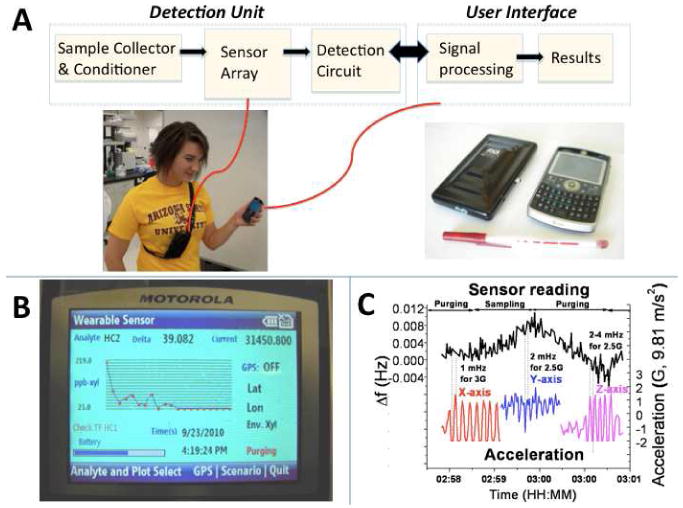
(A) Sensor components, and pictures. It shows a person wearing the detection unit near the breathing zone while holding the phone that acts as user interface, as well as a view of both VOC sensor components. (B) User interface on the phone, displaying the data received from the monitor. (C) Robustness test: the plot shows the sensor response (at 1-Hz data resolution) during x-, y-, and z- acceleration events detected with an accelerometer attached to the VOC sensor.

2. Material and Methods

2.1 Sensor Characteristics

General Characteristics

The VOC sensor has been developed to be wireless and wearable in order to record personal exposure levels and to suit many different conditions and scenarios. It weighs less than 0.7 lbs. and is not much larger than today's smart phones. This small size allows the user to either wear or hold the sensor depending on the application. The sensor has undergone stability tests to ensure robust functionality. Acceleration changes of up to 3 G's do not produce any detectable perturbation in the sensor's signal above the expected noise level range (Fig. 1C). The monitoring system is composed of two major components: the detection unit and the user interface (Fig. 1A).

Detection Unit

The detection unit contains three separate components: the sample collector and conditioner, the sensor array, and the detection circuit (Fig. 1A). The sample collector and conditioner subsystem cycles between sampling and purging periods, giving one data point per cycle. These sampling and purging time periods are adjustable; however, for the applications presented in this work, the sensor is calibrated for one minute of sampling followed by two minutes of purging, producing one data point every three minutes. This guarantees the accuracy of the sensor response by ensuring a well-defined baseline during the two-minute purging period. These conditions allow a detection limit of single digits part-per-billion by volume (ppb) range. In addition, the entire system has also been optimized with filters and tubing to avoid false responses from chemical interferences, like humidity and many common gases (Supporting Information, Section 3, page 3). The system optimization has been described elsewhere (Tsow, et al. 2009; Negi, et al. 2011). The sensor array is composed of micro-fabricated tuning forks within the sensor cartridge, which is designed so that it can be removed, altered or adjusted, and re-inserted directly via pins on the circuit board. The tuning forks have been specifically modified with high surface to volume ratio sensing material based on a molecularly imprinted polymer (MIP), created at ASU, with high selectivity towards total hydrocarbons (alkyl, aromatic and chlorinated hydrocarbons) (Iglesias, et al. 2009; Negi, et al. 2011). The characterization and performance of the MIP sensing material has been previously reported (Iglesias, et al. 2009; Negi, et al. 2011). The detection circuitry is based on a high-resolution frequency counter and has been optimized in order to achieve low noise levels of less than 0.2 mHz (at 0.2-Hz data resolution) (Fig. 1C). The combination of high aspect ratio materials and low noise levels maximizes the sensitivity of the sensor, and allows detection limits in the ppb range. An additional feature that improves the accuracy of the sensor is the integration of an onboard temperature sensor. This feature utilizes the microcontroller circuit to detect the temperature of the unit. A calculated relation between the unit temperature and the actual temperature in ambient conditions calibrates the on-board temperature (Supporting Information, Section 2, page 3). This temperature is used to adjust the tuning fork responses and allow proper functionality in temperature-varying environments.

Rechargeable Li-ion polymer batteries power the wearable detection unit. These batteries provide the system with sufficient power to operate the unit for over 10 hours continuously. The VOC sensor must be charged after each use using a standard AC power supply. Because of the small size and weight of the sampling unit, the VOC sensor can be either worn (as described in section 3.2 Field Evaluations) or carried by the user. The detection unit detects the sensing elements' responses and sends the raw data through Bluetooth^® to the user interface every second as long as the VOC sensor is within the range of the Bluetooth^® (∼ 600 feet).

User Interface

The user interface of the sensor is in a smart phone. A specific application in the smart phone has been developed to receive data from the detection unit, process the information, and display the results as shown in Fig. 1B. This graphic user interface has been designed for usability and variability, so that anyone can use it in a variety of situations. The interface displays information concerning the status of the detection unit, whether it is sampling or purging, as well as the correct functional status of the sensor array components. The data is shown as a plot, which can display the raw data as sensor counts versus time or processed data as concentration versus time. The graphic user interface allows the user to switch between these graphs or select other options, including which tuning fork sensor from the array to display. The user can fine tune the concentration plots to be displayed by selecting specific scenarios and settings, including industrial solvent concentration, and environmental or indoors environments, with readings in ppb-ppm for a specific hydrocarbon, and ppmC of hydrocarbons, respectively. In utilizing a smart phone as a user interface, the VOC sensor is also able to access GPS, which can be turned on at any time by the user. This allows the sensor system to provide temporal and spatial resolution in the collected results. All of the data that is monitored by the smart phone is stored in a text file so that it can later be downloaded onto a computer for further analysis, and eventually used to reconstruct the individual exposures via animated map videos.

2.2 Sensor Specifications

The entire system has been developed to achieve optimal results. Table 1 summarizes the specifications of the VOC sensor. The system, as presented here, primarily detects hydrocarbon gases, including aromatic, alkyl and chlorinated hydrocarbons, with a measurement range from 4 ppb detection limit up to 1 part per million by volume (ppm) for environmental settings and from 1 ppm up to 1000 ppm for industrial settings. These scenarios have different ranges due to different calibration factors needed for each environment. The different calibration factors utilize Langmuir-like isotherm equations with a higher affinity constant for lower concentration analysis (environmental settings), and a lower affinity constant for higher concentration analysis (industrial settings). The user is able to switch between the settings at any time by selecting the desired scenario on the smart phone application.

Table 1. Specifications of VOC sensor operation performance.

Gas Detected	Hydrocarbons
Measurement Range	Environmental: 0-1ppm
	Industrial: 1-1000ppm
Expected Operating Life	Valve: 5 years (minimum)
	Battery cycle life: Pump–up to 500 times Circuit–more than 300 times
Temperature Range	40°F to 115°F (5°C to 45°C)
Humidity Range	0 to 100% relative humidity (non-condensing)
Response Time	Raw Data: 1 second per measurement
	Calibrated concentration: 3 minutes per data point (adjustable)
Accuracy	±4% of measured value or better
Repeatability	3% of signal
Shock Resistance	±20 m/s2 (approximately ±2 G's) in x, y, and z axis
Calibration Frequency	Required: 1 month
	Recommended: 2 weeks
Calibration Gas	1 ppm Xylene

The sensing array is calibrated with 1-ppm xylene gas and, although it is recommended that the sensor be calibrated every two weeks, the required calibration time is 1 month. The sensor accurately performs in a temperature and humidity range of 40°F to 115°F (5°C to 46°C), and 10 to 100% (non-condensing), respectively. Calibration of the tuning fork outside the stated range has not been further studied, and needs to be determined. The accuracy of the sensor, when tested with artificial single hydrocarbon samples (e.g. xylenes), is better than ± 4% of the measured value, exemplifying the optimal performance of the complete system. The selectivity of the VOC sensor allows the detection of hydrocarbons, even in the presence of common interferents. Table 2 shows a list of these potential interferents and the sensors response to these compounds.

Table 2. Potential Interferences.

Table showing the sensor's response to common interferents.

Tested Interferent	Concentration Tested	Xylene Equivalent Response
Ethanol	42.3 ppm	0.0 ppm
Acetone	42.3 ppm	0.0 ppm
Dowanal	390.0 ppm	0.0 ppm
Isopropanol	42.3 ppm	0.0 ppm
Ammonia	20.0 ppm	0.0 ppm
Aniline	42.3 ppm	0.0 ppm
Benzyl acetate	150.0 ppm	0.0 ppm
Cyclohexane	42.3 ppm	42.3 ppm
Mist (perfume)	2-5% vapor	0.0 ppm

2.3 Experimental Methods

A number of field evaluation tests were completed with the total VOC sensor. The purpose of these experiments was to calibrate and validate the VOC sensor and verify its performance in real-world situations. The validation and calibration trials utilized reference methods and commercial sensors for comparison. The VOC sensor was either run side by side with a commercial sensor or with an air pump (model T2-03 DC, Parker, Cleveland, OH) running in ambient air and collecting samples in Tedlar bags (Environmental Sampling Supply, Oakland, CA), which were subsequently taken to a stationary instrument in the lab to be analyzed by a reference method.

Field test studies included indoor air quality monitoring during remodeling; personal exposure assessment in traffic areas; outdoor air quality at national and international locations; and various work environments and scenarios. For comparison, the EPA has reported long-term risk levels of 0.05 ppm for benzene, 0.1 ppm for toluene, and 0.1 ppm for xylene (Benzene, 2008; Toluene, 2007; Xylenes, 2007). In addition, OSHA has published permitted exposure levels (PEL) for benzene, toluene, and xylenes that are above 1 ppm (OSHA 2011). The levels of benzene, toluene, and xylenes in the environmental samples analyzed during this work were usually well below the EPA's and OSHA's adverse effect reported levels. However, other hydrocarbons in the environment accumulate and typically provide total hydrocarbon concentrations in the range of tens of ppmC (part-per-million Carbon, a concentration unit used to evaluate overall exposure from total hydrocarbons (see below, and more details in Supporting information, Section 1, Calibration of the VOC sensor, and Section 3. Field Testing, Exposure while travelling). Results from the ASU VOC sensor ranged from 0 ppmC, the equivalent of clean air observed in non-urban areas, to 50 ppmC in heavy traffic areas of a populated city, such as Los Angeles. The dynamic range of the readings allows accurate and reliable sensing and reporting of multiple compounds in a variety of environments.

2.3.1 Sensor calibration

Since outdoor and indoor personal environments have significantly different VOC distributions and sources, calibration factors (see below) tailored for the hydrocarbon distribution of both indoor and outdoor environments were used to ensure reliable results. More specifically, the VOC sensor was calibrated to read total hydrocarbon concentrations for two different conditions: outdoor environment with motor vehicle exhausts (MVE), and indoor air quality (IAQ). The calibration factors were obtained as follows. First, we determined the hydrocarbon distribution for outdoor (e.g., traffic) and indoor environments, using well-known literature data for MVE and IAQ, respectively (Brown, Frankel et al. 2007) (Weisel, Zhang et al. 2005), and further corroboration by Gas Chromatography-Flame Ionization Detection (GC-FID) analysis (CARB) and Selected Ion Flow Tube-Mass Spectrometry (SIFT-MS) (see below). Second, we calculated the calibration factors by adding the fractional sensitivity contributions of the hydrocarbons constituents of the environment mixtures (Supporting Information, Section 1, pages 1-2), according to:

$$S_{\mathit{\text{MVE}}}=\sum _{i=0}^n{S}_i\times X_i$$

$$S_{\mathit{\text{IAQ}}}=\sum _{i=0}^n{S}_i\times X_i$$

where S_MVE and S_IAQ are the sensitivity calibration factors for MVE and IAQ, respectively; S_i is the sensitivity of the sensor to each individual hydrocarbon which is a component of MVE or IAQ mixture, and X_i is the fraction of the hydrocarbon in the MVE or IAQ mixture. The X_i values were calculated based on concentrations of part-per-billion by volume (ppb), and the total concentration of hydrocarbons in ppb. The S_i values were determined as the ratio of number of counts from the sensor over the hydrocarbon concentration in ppb carbon (ppbC = ppb × number of carbons). As a consequence of the nature of the sensitivity factor (counts/ppbC), the total hydrocarbon concentrations were calculated as parts per billion Carbon (ppbC) to account for all carbons present in the mixture. Finally, the total hydrocarbon concentrations were reported as output result of the VOC sensor.

2.3.2 Validation Methods

Validation with reference methods

Laboratory evaluations were completed for validation purposes, using Gas Chromatography – Mass Spectrometry (GC-MS) and Selected Ion Flow Tube – Mass Spectrometry (SIFT-MS; Profile 3, Instrument Science Ltd, UK) (Smith, Diskin et al. 2001). The validation of the VOC sensor by GC-MS was presented in a former publication (Negi, Tsow et al. 2011) (for more details, the GC-MS method is described below in section 2.3.3, Field test methods, Case III). The VOC sensor validation results by SIFT-MS are presented here. While GC-MS allowed the sensor calibration and validation for complex environments with mixtures of hydrocarbons such as traffic exposure, SIFT-MS enabled calibration and validation of the VOC sensor under VOC sensor compatible conditions, providing real-time concentration readings. To validate the sensor with the SIFT-MS in the lab, xylenes standard samples were created, and tested on the SIFT-MS and in parallel with the sensor. In addition, indoor air samples from different rooms throughout ASU campus were collected, and the results assessed by SIFT-MS were correlated with the results assessed with the VOC sensor to determine the accuracy of the VOC sensor. Special attention was paid to collect samples at the same time and location as the VOC sensor to ensure similar air environments would be compared.

Inter-laboratory validation

Despite the fact that inter-laboratory validation of the VOC sensor had been reported before for occupational and safety applications (Negi, et al. 2011), validation for personal environmental studies, which are the focus of this work, were performed in this study with the Air Quality Department (AQDX) at Maricopa County, AZ.

In validation studies with ADQX, the ASU sensor results were compared with results from AQDX's mobile unit (Fig. 2B). The analysis of the real samples by the mobile unit was performed following a method from California Air Resources Board (CARB) (SOP No. MLD 032) (CARB). The method is a GC method that uses dual capillary columns and Flame Ionization Detection (GC-FID) for the determination of non-methane organic compounds in ambient air (method 2002). It has been derived and developed from an EPA compendium method for toxic organics (TO-14), and it is used daily by AQDX, Maricopa, AZ.

Fig. 2. Calibration and validation of the VOC sensor.

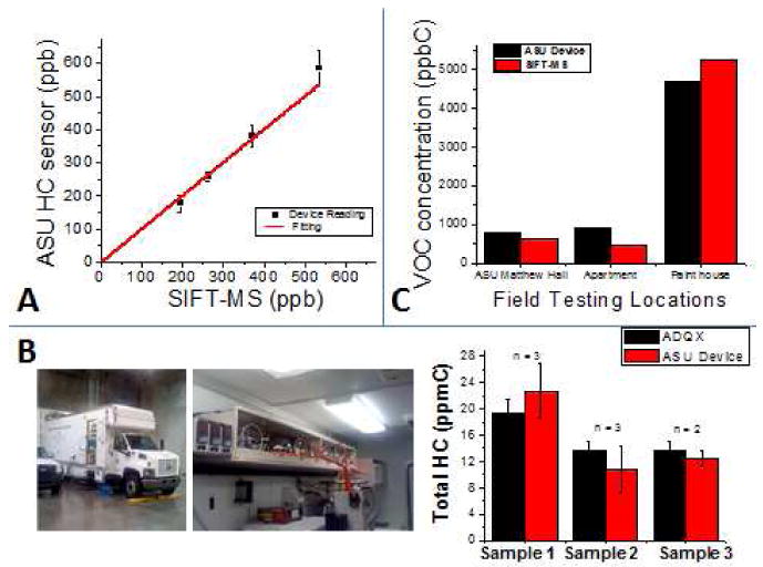
The sensor was calibrated and validated using the SIFT-MS and AQDX as standards for comparison. (A) Intra-laboratory sensor calibration and validation with SIFT-MS, using artificial samples of xylenes (n =3). The VOC sensor shows good correlation with the SIFT-MS, with a slope of 1.05, error of 3% at 95% CI. (B) VOC sensor validation with AQDX for outdoor environments. Comparative plot of total hydrocarbon readings from the ASU VOC sensor versus the results from ADQX. The number of times each sample was analyzed is shown in the plot. These tests sampled outdoor locations and show results that are in agreement. (C) VOC sensor validation with SIFT-MS for indoor environments. Comparative plot of total hydrocarbon readings from the ASU VOC sensor versus the results from SIFT-MS in samples taken from various indoor testing locations.

Validation with commercial VOC monitor

As a part of validation studies, the VOC sensor was compared to a commercial photo-ionization (PID) detection device (10.6-eV lamp). Note the brand of the instrument is not provided to avoid conflict with manufacturer. Both systems, VOC sensor and PID detection device, were used with a commercial benzene separation tube made of chromate salt, which extracts benzene from a given sample so that only benzene levels are analyzed by the system detector. The VOC sensor and PID detection device were tested against ambient air samples with concentrations of benzene determined by NIOSH 1501 modified method (NIOSH 2011), which involved collection of samples in coconut shell charcoal tubes (100/50 mg, SKC, Eighty Four, PA) and analysis by GC-MS by a 3^rd-party laboratory (Travelers, Industrial Hygiene Laboratories, Windsor, CT).

2.3.3 Field Test Methods

In order to demonstrate the use of the VOC sensor, field tests were completed for indoor and outdoor exposure assessment. Three examples are described below and additional examples can be found in Supporting Information (Section 3, pages 4-9).

Case I: Indoor Air Quality While Remodeling

Exposure profiles as a function of location and time were examined during paint remodeling. The VOC concentrations at different locations within a garage were assessed before and one hour after painting the floor with an interior paint (Glidden). The garage (10m × 12m × 3m) was closed for one hour prior to the test, and remained closed during the testing period. After the first test (“before painting”), the floor was painted with a single layer of paint using a paintbrush roll. The concentration of VOCs was assessed one hour later. The VOC sensor analyzed samples at locations with varying distances from the painted floor and a paint remover can (Klean-Strip, adhesive remover), which was present on a shelf above the painted area. In parallel, air samples were collected in Tedlar bags and taken immediately to the author's laboratory for analysis with SIFT-MS.

Case II: Outdoor Traffic Exposure

Several traffic exposure tests were performed in the Phoenix and Los Angeles areas as well as other parts of US and cities in the world (i.e., Nogales, Mexico and London, UK). It has been shown that high traffic areas have high levels of VOCs in the form of hydrocarbons, as cars release these compounds from the use of gasoline or diesel and incomplete combustion (Brown, et al. 2007). By using GPS capabilities of the VOC sensor, VOC concentration maps and movies showing temporal and spatial resolution of VOCs were created. To test the traffic levels in various cities, the user either wore the sensor near the user's breathing zone or left the sensor next to the car window, which was open. In the case of results presented in section 3.2 Field Testing, the VOC sensor inlet was pointing out of the car, and held next to the open car window to sense air from outside of the car. The car was a gasoline car, Toyota, Matrix 2005, whose exhaust was tested and proved to be negative for emissions of CO (0 ppm, Gas filter correlation CO Analyzer, Model 300E, Teledyne Instruments, Advanced pollution instrumentation, San Diego, CA). This test corroborated the full combustion of gasoline, and precluded any potential false positive reading in the VOC sensor due to the car itself. The car was driven at 30-60 miles per hour during the test. The VOC sensor was able to analyze the samples from the outdoor air and give the results of the personal exposure to a person driving through traffic. From the traffic data that was collected, hydrocarbon concentration maps (as mentioned previously) were produced. In addition, readings from the VOC sensor obtained for a period of ∼2 hours in areas near Phoenix, Los Angeles, and San Diego downtown were averaged and compared to pollution relative scale levels reported in www.airnow.gov for those specific areas on the test date.

Case III: Working Environments and Man Made Disasters

In order to examine specific work environments and man-made disasters, the exposure levels from the Deepwater Horizon's Oil Spill were explored in June of 2010. Two VOC sensors were taken to test the bays near New Orleans that had been suddenly exposed to oil from a nearby oil spill in the Gulf of Mexico. These bays are uninhabited by human beings and had not been exposed to hydrocarbon pollution prior to the oil spill. The VOC sensors were set up on a shrimp boat, which travelled into multiple bays about 60 miles from the oil rig where the spill had occurred. Under normal conditions, the air from these areas is expected to be essentially VOC free, with anticipated concentrations close to 0 ppm. In fact, similar non-polluted area tested by our VOC sensor (Mission bay, San Diego area next to sea) indicated readings of 0 ppmC. Two VOC sensors were used at different locations on the boat: one at the front and one near the middle of the boat. The two VOC sensors were located at least 30 feet away from the boat engine exhaust to minimize potential contamination from the exhaust of the engine. Also, a water sample was taken from Bay Batiste, Louisiana, so that the headspace of the water was analyzed using GC-MS (Supporting Information, Section 3, pages 5-6). The GC-MS method was optimized for detecting low-concentration aromatic and aliphatic hydrocarbons. The hydrocarbons in the sample were preconcentrated in a 100-μm polydimethylsiloxane coated solid phase microextraction fiber (SPME) for a period of 1 hour, and then placed into a 0.75-mm diameter glass injector. The hydrocarbons adsorbed in the SPME fiber were released in the GC injector by raising the temperature to 290 °C. The separation used 30 m, 250 μm, 0.25 μm HP-5 MS capillary column coated with 5% phenyl methyl siloxane. The analysis started with the temperature set at 40 °C. After 2 min, the column temperature was raised to 100 °C at 41 °C/min and then to 295 °C at 10 °C/min. The entire sample analysis lasted ∼38min. Identification of the analytes was performed using known standards and the mass spectrum library from NIST (AMDIS32 software). The total hydrocarbon level was obtained by adding up the individual hydrocarbons determined from the chromatogram, which was used to compare the readings of the VOC sensor.

3. Results and Discussion

3.1 Calibration and Analytical Validation

Comparison of VOC sensor with reference methods

In order to calibrate and validate the VOC sensor, GC-MS (Negi, Tsow et al. 2011) and SIFT-MS method were used. The correlation parameters of the VOC sensor assessed with SIFT-MS matched those assessed with GC-MS methods (accuracy within 95–105%, error ∼ 2%, and correlation coefficient (r²) > 0.9977) (Negi, et al. 2011). Correlation plots of readings from the VOC sensor versus SIFT-MS have the following features: slope ∼1.05, standard deviation ∼0.03, and r² > 0.999 (Fig. 2A). In addition, t-paired test of results assessed with the VOC sensor and the SIFT-MS also indicated good correlation (Table 3). The excellent correlation results were indicative of the high accuracy of the VOC sensor at intra-laboratory level. Additional validation at inter-laboratory level was also performed.

Table 3. Statistical Analysis.

t-Test to determine significant differences between the VOC sensor and reference methods

Validation Test	VOC Sensora	Reference Method	t-test	Significant Difference (p = 0.05)
SIFT - MS
Sample 1 (n=3)	195	177	-1.247	NO
Sample 2 (n=3)	264	259	-0.346	NO
Sample 3 (n=3)	371	382	0.762	NO
Sample 4 (n=3)	535	585	1.575	NO
GC-FID
Sample 1 (n=3)	22	19.4	-1.098	NO
Sample 2 (n=3)	10.8	13.6	1.183	NO
Sample 3 (n=2)	12.5	13.6	1.296	NO

^aconcentration of VOC in ppb xylenes for SIFT-MS (Selected ion flow – mass spectrometry), and ppbC for GC-FID (Gas chromatography – flame ionization detection), AQDX method; n: number of readings per sample.

In addition, validation for indoor air quality exposure measures was completed, using SIFT-MS (Fig. 2C) and indoor air samples obtained from various environments. The concentration levels of individual indoor air hydrocarbons detected by SIFT-MS were added to be compared with the total hydrocarbon response from the VOC sensor. As observed in Fig. 2C, VOC sensor readings from indoor environments showed readings with correlation factors of nearly one (Kaplan and Pesce 1989) from SIFT-MS. In summary, the VOC sensor delivered quality and valid results when compared with reference methods.

Validation with Air Quality Department in Arizona

Inter-laboratory validation for environmental applications was completed in collaboration with AQDX. By following the procedure described in the section Materials and Methods, 2.3.1 Sensor calibration, total hydrocarbon concentrations (as ppmC) were determined and calculated from all measured short and mid-range hydrocarbons (C2-C12). Once the total hydrocarbon concentrations from the GC-FID method were obtained, they were compared to the readings of total hydrocarbons from the calibrated VOC sensor. The total hydrocarbon readings from our VOC sensor matched the results from the AQDX mobile unit (Fig. 2B). Accuracy factors > 84% between the VOC sensor and the mobile unit's results demonstrated the VOC sensor's capability to produce reliable measurements in outdoor environments.

Comparison of VOC sensor with commercial device

The VOC sensor was compared to commercially available PID detection device for detection of benzene under the conditions specified in the section materials and methods. While the VOC sensor was able to provide benzene readings of artificial calibration samples (n=5) in the range of (100-200) ppb and real samples (n=3) in the range of (226 ± 71) ppb, the PID device did not detect the presence of benzene and indicated null readings (0.0 ppm) for both artificial calibration samples and real samples. These tests indicated the superior detection limit of the VOC sensor than that of the commercial PID device. In addition, comparison of VOC sensor readings with readings from NIOSH 1501 modified method for analysis of benzene by a 3^rd party laboratory was performed. Real samples (n=3) analyzed by NIOSH method with (275 ± 35) ppb benzene levels, indicated an accuracy higher than 81% for the VOC sensor compared with NIOSH 1501 modified method. It is worth noticing that while the VOC sensor provided real-time results, NIOSH method required of sample collection tube shipping and several days of waiting time until the results were available. Further efforts to improve the VOC sensor accuracy and statistically significance of correlation of VOC sensor results with reference methods are on going. Disposable sensor cartridges are under development to increase the sensor calibration accuracy.

3.2 Field Testing

Case I: Indoor Air Quality While Remodeling

Indoor air often has higher levels of VOCs due to the quantity of products emitting toxic chemicals that are used in homes and to the containment of these chemicals within the enclosed space with a lack of ventilation in comparison to that of an outdoor environment. In this regard, the profiles of VOC concentration due to painting were investigated. Measurements were taken at different locations in a garage before and after painting the floor. The relationship between the VOC concentrations and the sampling location is summarized in Fig. 3A-B. As expected, the results showed that the VOC levels are significantly higher after painting and near the VOC sources (e.g., paint remover container). The concentrations were contained within the garage as the paint and solvent released VOCs and led to accumulation of the hydrocarbons to significantly higher exposure levels. These findings underline the importance of personal exposure with high spatial and temporal resolution. In this particular case, they allowed accurate determination of paint curing time and identify safer exposure locations.

Fig. 3. VOC distribution before and after a floor painting activity.

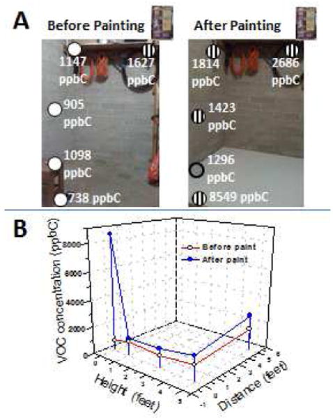
The location of the samples taken are marked in (A). Relatively high, medium, and low concentrations are shown in striped, gray solid, and white circles, respectively. Samples were taken before painting and then one hour after painting. The exposure levels are higher near the sources of the VOCs: floor, and a paint remover can located on top of a shelf. (B) Plot showing the VOC concentrations as a function of height and distance from the painted floor and a paint remover can.

Case II: Outdoor Traffic Exposure

The portability and robustness of the VOC sensor allowed the sensor to be used in various conditions and locations. One such possible application of the wearable sensor was traffic monitoring. Multiple locations with varying amounts of traffic in the Phoenix area were tested using the sensor. After testing, a map of the total hydrocarbon concentrations was created and is shown in Fig. 4A. It was observed that the hydrocarbon levels monotonically decreased with the distance from the portion of the route that had the highest traffic density (Highway 202 and Mill Ave. cross-section, Tempe, AZ) (Fig. 4B). As expected, lower traffic areas such as Papago Park and ASU campus presented significantly lower hydrocarbon levels than the highway (see video in the supporting information with personal exposure assessment throughout the test route, Supporting Information-partII.m4v). In addition, field tests in different cities were performed (see Section 3, Supporting information, page 9), and confirmed that personal exposure is highly dependent upon location, environment, and city. Given the data presented, the need for personal monitors to assess these various situations is emphasized, exemplifying the importance of cost efficient, versatile, portable exposure monitors to capture these differences.

Fig. 4. Assessment of total hydrocarbons from traffic.

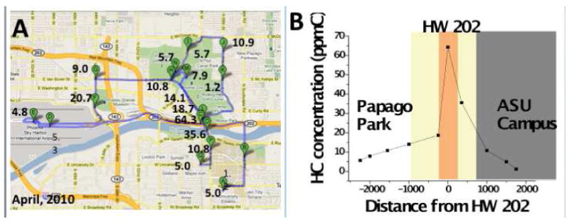
(A) Route taken around the Phoenix area. The numbers on the map show the concentrations of total hydrocarbon exposure in ppmC. (B) Hydrocarbon profile across lateral section of highway 202. The plot illustrates how the hydrocarbon concentration increases closer to the high traffic highway and decreases as the distance from the highway (in meters) increases.

Case III: Working Environments and Man Made Disasters

As previously explained in the section Material and Methods, Field test methods, environments affected by the 2010 BP Oil spill were tested (Fig. 5A). As previously explained, the concentrations in these areas were expected to be close to 0 ppm. However, due to the presence of the oil, the levels of exposure were similar to the levels found in a populated city (Fig. 5B). The VOC sensor readings were found to be highly dependent upon the location and wind conditions. As shown in Fig. 5C (and Supporting Information-partIII.m4v), the VOC sensors detected exposure levels up to 6 ppmC in Bay Batiste, Louisiana, where both the highest and the lowest hydrocarbon levels were detected. These results emphasize the significance of exposure detection that is real-time and at a personal level, as these spikes in concentration may have been missed or averaged away with the low concentrations by another monitor in nearby EPA monitoring stations (see more details in Supporting Information, Section 3, page 5).

Fig. 5. Hydrocarbon assessment in the 2010 Deepwater Horizon's oil spill.

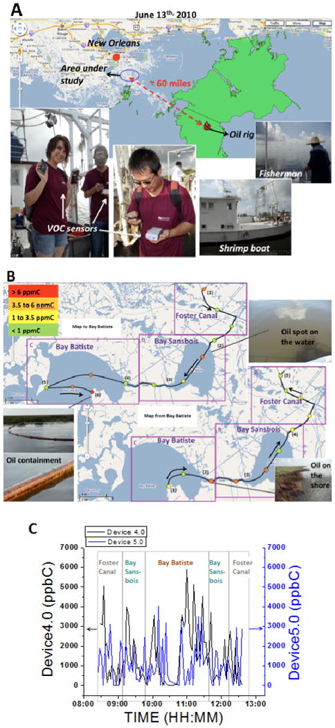
(A) Map (source: Google maps) showing the testing location approximately 60 miles from the source of the oil spill, and pictures of VOC sensors and testing conditions. (B) Hydrocarbon concentration map and route that was taken along the boat trip. One may note that both high and low concentrations are detected in Bay Batiste and that the levels do not remain the same on the way back to Foster Canal as on the way in to Bay Batiste. (C) Hydrocarbon concentration vs. time through the trip obtained from two VOC sensors (VOC sensor 4.0 and VOC sensor 5.0) that were located at different locations on the boat.

In addition, GC-MS analysis was conducted on water samples collected in the area. A water sample was taken in order to use the headspace to test the air quality for comparison purposes. It was found that the headspace contained long alkyl hydrocarbons and their derivatives. The concentration levels were consistent with the averaged levels for the real-time VOC sensor results (Supporting Information, Section 3, pages 5-6). These lower volatility compounds are likely to be dominant because many of the high volatility components of petroleum (e.g., benzene, toluene, ethylbenzene, and xylenes not detected in the samples taken from shore) may have been lost in the traveling oil sheet.

4. Conclusions

In summary, ASU's VOC sensor is highly portable, robust, easy to operate, and correlates well or outperforms similar commercial VOC sensors (i.e. PID). This VOC sensor has been developed for optimal performance concerning sensitivity, selectivity, portability, and usability. The sensor detected higher exposure of hydrocarbons in high traffic outdoor areas, inside remodeled rooms or near chemical emitting products, and in man-made disasters. The sensors provided an accuracy higher than 81% and consistency that is needed in addition to the benefits of being wearable and offering real-time results (one reading every three minutes) without false responses from interferences in a wide detection range of ∼ 4ppb to 1000 ppm. The noted attributes and the findings that have been presented indicate that the sensor developed at ASU is suitable for indoor and outdoor environmental personal exposure studies, and has the potential to greatly improve our knowledge of personal exposures and to help protect human health as well as the environment. In addition, the VOC sensor requires little training to operate, thus allowing population studies in the hands of ordinary users or researchers.

References

- 1.(2007). Toluene, U.S. Environmental Protection Agency. 2011: Hazard Summary of Toluene.
- 2.(2007). Xylenes (Mixed Isomers), U.S. Environmental Protection Agency. 2011: Hazard Summary of Xylenes
- 3.(2008). Benzene, U.S. Environmental Protection Agency. 2011: Hazard Summary of Benzene.
- 4.Blasco C, Pico Y. Prospects for combining chemical and biological methods for integrated environmental assessment. Trends in Analytical Chemistry. 2009;28(6):745–757. [Google Scholar]
- 5.Brown SG, Frankel A, et al. Source apportionment of VOCs in the Los Angeles area using positive matrix factorization. Atmospheric Environment. 2007;41:227–237. [Google Scholar]
- 6.Byrne R, Diamond D. Chemo/bio-sensor networks. Nature Materials. 2006;5(6):421–424. doi: 10.1038/nmat1661. [DOI] [PubMed] [Google Scholar]
- 7.CARB. Method from California Air Resources Board. The method is a GC method that uses dual capillary columns and Flame Ionization Detection (GC-FID) for the determination of non-methane organic compounds in ambient air. It is developed from an EPA compendium method for toxic organics (TO-14), and it is used daily by AQDX, Maricopa. SOP No MLD 032 [Google Scholar]
- 8.Diamond D, Coyle S, et al. Wireless sensor networks and chemo-/biosensing. Chemical Reviews. 2008;108(2):652–679. doi: 10.1021/cr0681187. [DOI] [PubMed] [Google Scholar]
- 9.Diamond D, Lau KT, et al. Integration of analytical measurements and wireless communications--Current issues and future strategies. Talanta. 2008;75(3):606. doi: 10.1016/j.talanta.2007.11.022. [DOI] [PubMed] [Google Scholar]
- 10.Etzel RA. Air pollution and bronchitic symptoms in southern California children with asthma. Environmental Health Perspectives. 1999;107(9):691–691. doi: 10.1289/ehp.107-1566463. [DOI] [PMC free article] [PubMed] [Google Scholar]
- 11.Fent KW, Evans DE. Assessing the risk to firefighters from chemical vapors and gases during vehicle fire suppression. Journal Of Environmental Monitoring. 13(3):536–543. doi: 10.1039/c0em00591f. [DOI] [PubMed] [Google Scholar]
- 12.Iglesias RA, Tsow F, et al. Hybrid Separation and Detection Device for Analysis of Benzene, Toluene, Ethylbenzene, and Xylenes in Complex Samples. Analytical Chemistry. 2009;81(21):8930–8935. doi: 10.1021/ac9015769. [DOI] [PMC free article] [PubMed] [Google Scholar]
- 13.Kaplan AK, Pesce AJE. Clinical Chemistry: Theory, Analysis, Correlation. Mosby, Inc.; 1989. [Google Scholar]
- 14.McConnell R, Berhane K, et al. Traffic, susceptibility, and childhood asthma. Environmental Health Perspectives. 2006;114(5):766–772. doi: 10.1289/ehp.8594. [DOI] [PMC free article] [PubMed] [Google Scholar]
- 15.method CE. Standard operating procedure for the determination of non-methane organic compounds in ambient air by gas chromatography using dual capillary columns and flame ionization detection. 2002 Jan http://www.arb.ca.gov/aaqm/sop/sop032.pdf.
- 16.Negi I, Tsow F, et al. Novel monitor paradigm for real-time exposure assessment. J Expos Sci Environ Epidemiol. 2011;21(4):419–426. doi: 10.1038/jes.2010.35. [DOI] [PMC free article] [PubMed] [Google Scholar]
- 17.Nilson LN, Karlson B, et al. Delayed manifestations of CNS effects in formerly exposed printers - A 20-year follow-up. Neurotoxicology and Teratology. 2010;32(6):620–626. doi: 10.1016/j.ntt.2010.05.004. [DOI] [PubMed] [Google Scholar]
- 18.NIOSH. NIOSH 1501 modified method. 2011 http://www.cdc.gov/niosh/docs/2003-154/method-cas9.html.
- 19.OSHA. Ocuppational Safety and Health Administration - Chemical Sampling Information - Permited Exposure Levels of Chemicals. 2011 http://www.osha.gov/dts/chemicalsampling/toc/toc_chemsamp.html.
- 20.Pejcic B, Eadington P, et al. Environmental monitoring of hydrocarbons: A chemical sensor perspective. Environmental Science & Technology. 2007;41(18):6333–6342. doi: 10.1021/es0704535. [DOI] [PubMed] [Google Scholar]
- 21.Potyrailo RA, Morris WG. Multianalyte chemical identification and quantitation using a single radio frequency identification sensor. Analytical Chemistry. 2007;79(1):45–51. doi: 10.1021/ac061748o. [DOI] [PubMed] [Google Scholar]
- 22.Smith D, Diskin AM, et al. Concurrent use of H3O+, NO+, and O-2(+) precursor ions for the detection and quantification of diverse trace gases in the presence of air and breath by selected ion-flow tube mass spectrometry. International Journal Of Mass Spectrometry. 2001;209(1):81–97. [Google Scholar]
- 23.Tang WY, Ho SM. Epigenetic reprogramming and imprinting in origins of disease. Reviews in Endocrine & Metabolic Disorders. 2007;8(2):173–182. doi: 10.1007/s11154-007-9042-4. [DOI] [PMC free article] [PubMed] [Google Scholar]
- 24.Tsow F, Forzani E, et al. A Wearable and Wireless Sensor System for Real-Time Monitoring of Toxic Environmental Volatile Organic Compounds. Ieee Sensors Journal. 2009;9(12):1734–1740. [Google Scholar]
- 25.Weisel CP, Zhang J, et al. Relationships of Indoor, Outdoor, and Personal Air (RIOPA) Part I. Collection Methods and Descriptive Analyses, Health Effects Institute, Air Toxics Research Center. 2005 Nov; Report number 130. [PubMed] [Google Scholar]
- 26.Weisel CP, Zhang J, et al. Relationships of Indoor, Outdoor, and Personal Air (RIOPA); Part I Collection Methods and Descriptive Analyses, Health Effects Institute; Report. Air Toxics Research Center. 2005. Nov, 130. [PubMed] [Google Scholar]
Associated Data
This section collects any data citations, data availability statements, or supplementary materials included in this article.