Summarizing and correcting the GC content bias in high-throughput sequencing

Abstract

GC content bias describes the dependence between fragment count (read coverage) and GC content found in Illumina sequencing data. This bias can dominate the signal of interest for analyses that focus on measuring fragment abundance within a genome, such as copy number estimation (DNA-seq). The bias is not consistent between samples; and there is no consensus as to the best methods to remove it in a single sample. We analyze regularities in the GC bias patterns, and find a compact description for this unimodal curve family. It is the GC content of the full DNA fragment, not only the sequenced read, that most influences fragment count. This GC effect is unimodal: both GC-rich fragments and AT-rich fragments are underrepresented in the sequencing results. This empirical evidence strengthens the hypothesis that PCR is the most important cause of the GC bias. We propose a model that produces predictions at the base pair level, allowing strand-specific GC-effect correction regardless of the downstream smoothing or binning. These GC modeling considerations can inform other high-throughput sequencing analyses such as ChIP-seq and RNA-seq.

INTRODUCTION

Since it was introduced, Illumina Genome Analyzer high-throughput sequencing has become an increasingly popular technology for determining relative abundance of DNA in an assay. In this method, the DNA of interest is fragmented, and one or both ends of the fragment sequenced. These sequenced short reads, or read pairs, are aligned to a reference genome. Counts of aligned fragments may be used to measure DNA copy number (DNA-seq), protein binding (ChIP-Seq) or expression (in RNA-seq). In many of these assays, researchers would like to compare such fragment counts between different locations in the genome. It is therefore troubling that the number of reads mapped to a genomic region depends considerably on the sequence itself.

One well-documented (1) dependency is the GC content bias, that is between the proportion of G and C bases in a region and the count of fragments mapped to it. (We use ‘fragment count’, instead of ‘read count / read coverage’ because paired reads identify a fragment). This variability does not reflect the signal of interest, but might confound it. Since GC abundance is heterogeneous across the genome and often correlated with functionality, the GC effect can be hard to tell apart from the true signal. The effect does not decay even for larger bins: large (>2-fold) differences in coverage are common even in 100 kb bins (2). To make matters harder, the effect is not consistent between repeated experiments, or even libraries within the same experiment (see below). Estimating and directly correcting for this effect has become a well-established step in protocol design (3), quality control (http://picard.sourceforge.net/index.shtml) and studies (4,5) using high-throughput sequencing.

Most current correction methods follow a common path. Both fragment counts and GC counts are binned to a bin-size of choice. A curve describing the conditional mean fragment count per GC value is estimated (by binning, 5, or assuming smoothness 6, 7). The resulting GC curve determines a predicted count for each bin based on the bin's GC. These predictions can be used directly to normalize the original signal, or as the rates for a heterogeneous Poisson model. Bin size is arbitrarily set, usually to match downstream analysis. While these methods remove most of the GC effect, they do not use any prior knowledge about the effect. This is perhaps why key features of the GC curve, such as its unimodality, have sometimes been overlooked or completely missed in the estimation.

While GC effect is commonly corrected for, until recently studies regarding the nature of this bias have been rare. Dohm et al. (2008, 1) first described the effect of the GC on fragment coverage in Illumina GA. The effect they found seemed highly linear—fragment coverage increased with GC content, but they sequenced genomes that were GC poor. This is probably why the GC effect is sometimes described as the correlation between GC and coverage (8). In later high-throughput studies of the human genome, plots of GC curves usually reflect non-linear curves, but are rarely investigated further than non-parametric fitting. Identifying the source of the bias was also hard, because the composition of the DNA molecule can affect many stages of the protocol. Sequence-related biases in the priming (9), size selection (3), PCR (10) and probability of sequencing errors (11–13) have all been found. In a recent analysis (12), PCR was shown to play the dominant role in the stages before the sequencing. While sequencing protocols have partially evolved to accommodate this new understanding (10,12), estimation and correction methods have not.

From a technical point of view, the above sources of bias cluster according to the location and scale of GC that is thought to be driving the non-uniformity in the counts. Locally, GC counts could be associated with the stability of the DNA, and thus modify the probability of a fragmentation point occurring in the genome, leading to a ‘fragmentation model’. The GC content could primarily modify the base-sequencing process; we call this the ‘read model’, suggesting that the GC of the forward read (in the single-end) or both reads (in the paired-end case) best explain fragment count. ‘Full-fragment models’ assume that the GC of the whole fragment determines which fragments are selected or amplified. Finally, ‘global models’ refer to GC effects on scales larger than the fragment length, e.g. through an association with some higher order structure of the DNA. These loosely defined models can be realized statistically by counting the GC in a suitable region and comparing that to fragment coverage. While the differences between the above models might seem small, they are sometimes considerable (see below). Note that any GC bias removal strategy implicitly chooses a GC bias model when it uses GC in some region to correct for the effect.

In this work, we take a descriptive approach to investigating the common structures found in GC curves in DNA-seq. We study the effect of GC on fragment count in many DNA-sequencing copy number (CN) assays for (both normal and tumor) high-coverage human genomes, taken from multiple labs. CN for normal genomes should rarely change, and so observed variability in fragment count can almost always be attributed to technical effects rather than biological signal. We use a single position model to estimate the effect of GC on the fragment counts, and seek a parsimonious description for this family of curves. (The same model underlies the correction method BEADS, see ref. 14). Such a description has two main advantages: it allows more accurate estimation of the GC curve by highlighting an appropriate set of parameters; and it provides important empirical evidence regarding the experimental stages that may cause or modify this effect.

The data we analyze suggest that to a large extent, the dependence between count and GC originates from a biased representation of possible DNA fragments, with both high GC and high AT fragments being underrepresented. This global structure of the GC dependence is consistent, but the exact shape varies considerably across samples, even matched samples. We describe a parsimonious model for the GC effect, and show it suffices to predict the GC effect on fragment coverage on all scales, all chromosomes and for both strands. This prediction is better than generic fitting approaches currently used, as illustrated on DNA-seq with and without CN events. Our model produces single base pair prediction, allowing optimal correction regardless of the required downstream smoothing. Finally, this provides empirical evidence strengthening the hypothesis that PCR is the most important cause for GC bias.

MATERIALS AND METHODS

Mapped read files

The main data set we use consists of two samples of DNA from an ovarian cancer patient: one sample from the tumor and another normal sample (from white blood cells). Each of these DNA samples was turned into two separate fragment libraries, differing in fragment length distribution. Fragments were sequenced on both ends — 75 bp reads on each end—according to standard Illumina procedures. Each fragment was then mapped back to the human reference genome, based on the 5′ read. These sequenced read pairs were mapped to a reference using BWA (version 0.4.9, 15). Human genomes were mapped to NCBI build 36 version 3 (//ftp.ncbi.nih.gov/genomes). The data are available at the NCBI Sequence Read Archive under accession numbers SRX011739 (tumor) and SRX011777 (normal). Unless otherwise mentioned, all plots are from chromosome 1 (chr1) of normal Lib1. Additionally, we analyzed another sample from a breast tumor cell line (Figure 11); healthy genome libraries generated under optimized protocols (Supplementary Figures S5 and S6), and data from a ChIP sequencing experiment of Arabidopsis (Supplementary Figures S7 and S8). For details see Table 1 .

Figure 11.

GC plots for Dataset 2. (A) GC effect for 10 kb (chromosome 1). (B) TV scores for GC windows of different lengths with a = 0 (comparable to Figure 3). (C) GC curve at fragment model (W_2,500). (D) Observed (blue) and predicted (black) counts against GC for 10 kb bins (chromosome 2).

Table 1.

List of data sets analyzed in this article

Name	Type	Date	Institute	Fragmentsa (bp ± SD)	Reads (bp)
TCGA-13-0723
Normal Lib 1	Matched Normal	4/09	Wash U	154 ± 17	75
Normal Lib 2	Matched Normal	4/09	Wash U	284 ± 38	75
Tumor Lib 1	Ovarian Tumor	4/09	Wash U	173 ± 22	75
Tumor Lib 2	Ovarian Tumor	4/09	Wash U	293 ± 31	75
HCC1569	Breast Tumor	1/09	UC Berkeley	507 ± 40	45
SRX040660	Matched Normal	9/10	Broad	172 ± 19	101
SRX040661	Matched Normal	9/10	Broad	173 ± 19	101
ChIP Rep 1	Arabidopsis	7/09	UC Berkeley	100b	36
ChIP Rep 2	Arabidopsis	7/09	UC Berkeley	100b	36

Lib1 and Lib2 are from the same sample.

^aMedian and SD of fragment length are based on paired-end mapping where available, or ^blibrary preparation estimates otherwise.

For each library, this procedure resulted in a list of fragments. Each fragment can be described by the location of its 5′-end (chromosome, location and strand), and its length. Length was inferred from the mapping of the 3′-end, based on the paired-end alignment of BWA. Only those pairs in which the 5′ read was uniquely mapped were kept (flag XT:A:U of BWA), because allocation of reads mapped to multiple locations is very sensitive to the comprehensiveness of the reference. However, we did not discard a pair when the 3′ was not mapped; thus for most of this analysis, the fragment set is similar to that obtained from single-end data. Only where fragment length is explicitly discussed did we remove fragments when the 3′ was not mapped (∼1% of fragments). No additional quality filtering was applied.

Loess model

Previous analyses of GC focused on the relation between fragment count and GC composition for particular bin sizes (see, for example, ref. 6, 16). We call this the ‘loess model’, and describe shortly how we reproduce such estimation. For a given bin (interval of the genome), GC is the fraction of G and C bases in that bin according to the reference genome. Bin counts are the total number of (forward) fragments with 5′-end inside the bin. To account for uniqueness of sequences, a mappability measure is calculated for each position (base pair) in the bin. A location is called ‘mappable’ if the k-mer of the reference genome starting at the location is not perfectly repeated at any other location in the genome, where k is the read length [checked by a Python script using the Bowtie mapper (17)]. All subsequent analysis is done in R (18). The GC bias curve is determined by loess regression of count by GC (using the ‘loess’ R package) on a random sample of 10 000 high mappability (>0.9) bins. The smoothness parameter for the loess should be tuned to produce curves that are smooth but still capture the main trend in the data. We use 0.3 as the default value. The estimated rates for GC values with too few data points are set to 0.

Single position models

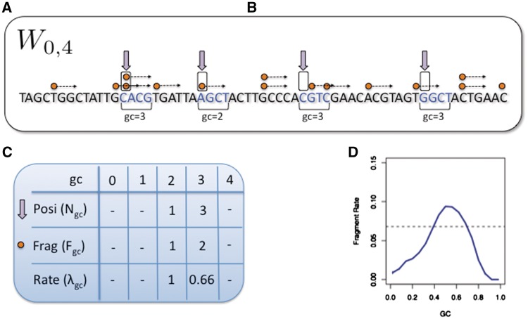
We call ‘single position models’ those models that estimate the ‘mean fragment count’ (the rate) for individual locations rather than bins. We consider a family of such models linking fragment count to GC, where the expected count of fragments starting (5′-end) at x depends on the GC count in a window that starts a bp from x. Figure 1 illustrates the case in which GC is computed from a 4-bp window starting at the fragment 5′-end. Each such model can be characterized by the shift a and the length l of its ‘driving’ GC window. W_a,l denotes the model in which the fragment count starting at x (5′-end) depends on the GC between x + a and x + a + l. (We will use GC(x + a, l) for the GC count of the l bp window starting at x + a). For example, in W_0,r the fragment count is determined by the GC of the first r bp of the fragment. The model W_a,l has l + 1 rate parameters, λ₀… λ_l, corresponding to windows with gc = 0,…,l.

Figure 1.

Single position model estimation. (A) Mappable positions along the genome are randomly sampled (⇓); (B) these positions are stratified by the GC count in the corresponding sliding window (here a = 0, l = 4); (C) the number of fragments (→) with 5′-end (○) in sampled locations are counted; (D) mean fragment rates for each stratum are estimated, taking the ratio between fragment count and positions in the stratum. These form the GC curve (here the curve for a = 75, l = 50 from Figure 4C).

The following is a description of our method of estimating the parameters for a single position model W_a,l. A large (n ≈ 10 million) random sample of mappable locations is taken from the genome. Large genomic regions with either zero fragment counts or with counts that are extremely high (>0.99 quantile + median) were removed from the sample. The sample is partitioned (stratified) according to the GC of the reference genome: if gc = GC(x + a, l) then position x is assigned to stratum S_gc. Let N_gc denote the number of sample positions assigned to S_gc. Note that the assignment to strata depends only on properties of the model and the reference genome, not on the sequencing data.

Next, for every value of gc, we count the total number F_gc of fragments starting (5′-end) at the x's in S_gc. We estimate λ_gc by taking the ratio

The random sample is taken over (potential) ‘positions’ in reference genome, not ‘fragments’. The estimated fragment rates implicitly account for the total number F of mapped fragments in the sample (). For large windows, we expect many strata to be small. Strata are then pooled together (constant jumps of 3 or 6 are used). The parameters that were skipped are then estimated by interpolation using loess regression (smoothness 0.2).

Comparing models

An estimated model W_a,l (i.e. each choice of GC window) can be used to generate predicted counts for any genomic region. Models can be compared based on the quality of their corrections (see below). However, this is very inefficient, and we consider a simpler surrogate measure that allows comparison of many different models regardless of window size. We use the normalized ‘total variation distance’ (TV) (19) between the stratified estimated rates (W_a,l) and a uniform rate (U, equal to the global mean rate in our sample )

The above (TV) score is a weighted L₁ distance from the global mean, divided by (so it will be between 0 and 1). In other words, it is the total variation distance between the empirical distribution for a single fragment (under specific GC categories) and a uniform distribution. Thus, it measures the proportion of fragments influenced by the stratification, and is comparable across data sets. We look for high TV, meaning counts are strongly dependent on GC under a particular stratification. This could indicate that correcting for such a model would best correct for the GC dependence.

Fragment length models

To measure the effect of fragment lengths, a separate single position model is fit for fragments of each length. accounts for the fragments of length s only. The locations in the sample are still partitioned according to gc, but instead of counting all fragments starting at x's in S_gc, only fragments of length s are counted (). Rates are estimated as before,

For the fragment length model, we would like to model the count of fragments using the GC in the fragment, after removing a few base pair from each end to reduce the impact of the local biases. Hence, the GC window size l becomes s − a − m. The model is then determined by a the shift from the fragment 5′-end, and m the margin from the 3′-end. 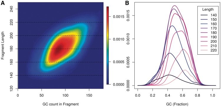( Note that if l had been instead fixed for any s, the set would be a refinement of W_a,l, with and . This is not the case here, because the GC window grows with the fragment length.) The parameters of this model are rates for each combination of fragment length and GC. The rate surface is smoothed using a 2D Gaussian kernel (θ = 0.7 for estimation, θ = 1.8 for visualization; Figure 5).

Figure 5.

Fragment rate by length and GC. (A) A heat map describes rates for each (GC, length) pair. Each dotted line represents a single length. In (B), GC curves for fragments of specific lengths are drawn [corresponding to the dotted lines in (A)]. Blue / dark curves represent shorter fragments than red / bright. Here x-axis is the fraction of GC. All fragment length models here have a margin of 2 from both fragment ends (a = 2, m = 2).

Predicted rates

The prediction of mean fragment count μ_x for genomic position x using W_a,l is

In essence we are ‘smoothing’ the observed fragment counts using W_a,l. That is, we are estimating the number of fragments at x under the model W_a,l, by the average of all such numbers found in x's with the same value of GC(x + a, l) (in our sample of mappable locations). Therefore, when we wish to remove, i.e. correct for the GC bias, as assessed by W_a,l at x, we would divide the observed number of fragments emanating from any x by μ_x. In practice, we rarely use the final correction at the single base pair resolution, but usually after aggregating into bins, see below.

For the fragment length model, , the predicted count of fragments from all lengths (if x is mappable) is the sum of predictions for each length

with c a scale factor to equalize predicted and observed total fragment counts (based on the fraction of fragments with unknown length). Finally, the mappability model uses the global mean () as the predictor for each mappable position

Fragment counts in bins are additive, so for any bin b the predictor is . The reverse strand follows similar fragment rates when the GC window direction is reversed (see below). To show this, we estimate the strands separately except where otherwise stated.

Evaluation

We evaluate the success of a model by comparing its predictions () to the vector of observed fragment counts (F). For robust evaluation, we measure the mean (average) absolute deviation (MAD) between predicted and observed counts. Let B be the set of bins, and F_b the count of fragments for which 5′-end is inside of bin b.

For visualization, observed counts are normalized by their respective predicted values, creating an implicit measure of copy number (CN). That is, we plot

where ϵ = 0.1 to stabilize this estimate when the predicted number of fragments is small. On non-tumor data, we expect these values to be concentrated ∼1, and the spread should indicate the quality of the predictions.

Comparisons with Poisson variation

Let F_b be the fragment count in bin b as before, μ_b the expected value of F_b assuming a Poisson distribution and an estimate of μ_b under some model W_a,l. We compare the variation of F_b around the predicted means to the variation expected under a Poisson distribution. Then the residual variance (RV) is

Under the heterogeneous Poisson, the RV is composed of a bias term, a term for estimation error and Poisson variance as following

where the first quantity is a bias term, corresponding to the goodness of fit of the model; the second is estimation error due to fitting the model, and should be relatively small; while the last is a measure of the pure Poisson variance, and whose value should be about the average of the μ_b.

Thus, RV measures how well a model captures the rate parameters, and cannot be less than the pure Poisson variance. We compare the RV of the mappability model (MR), and the RV of the fragment GC model (GR), to an independent estimate of the pure Poisson variance (). Extremely high counts [F_b > 0.99 quantile + median(F)] were removed from these.

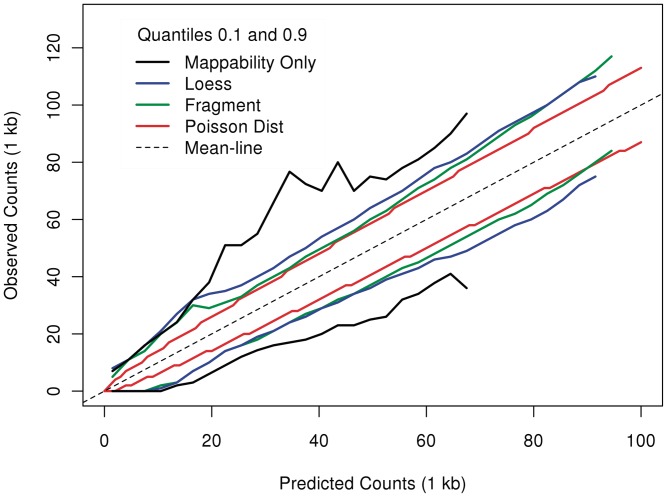
Although we remove extreme high counts, variances can still be influenced by a relatively small set of bins with high counts. We would like to compare residual variation of the different models in a way that is more robust to those. Following Ref. (20), we look at the empirical quantile curves. For a given model, we grouped counts from 1 kb bins according to their predictions 's). We computed for each group the observed 0.1 and 0.9 quantiles. Plotted against the estimated rate of the group, each quantile level forms a curve. The distance between the curves reflects the variation around predicted means. When this distance is considerably larger than that of the Poisson, this indicates that different rates were assigned to the same predicted value, meaning that much variation remains unexplained by the model.

Software and data availability

GCcorrect is an R package implementing exploratory analysis, estimation and correction methods for GC content effects, and is available for download from http://www.stat.berkeley.edu/~yuvalb.

RESULTS

Bin counts

The GC effect for human genomes is largely unimodal. In AT-rich regions, coverage increases with increasing GC. In GC-rich regions, coverage decreases with increasing GC. The peak coverage can be different for different data sets (and bin sizes), but is usually located between 0.4 to 0.55 GC. That 10 kb bins with GC > 0.5 are rare in the human genome is perhaps the reason for calling GC effect ‘linear’. This unimodal relation can be seen at almost any scale, from 50 bp to >100 kb. While in the AT-rich region the increase in coverage is quite linear with GC, it is less linear (and more variable) in GC-rich regions.

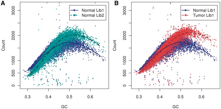
The curves of difference samples are all unimodal, but not the same: the slopes, location of mode and variance around the unimodal curves vary considerably between samples. Indeed, variability between curves is found not only between labs or protocols, but also between tumor and normal sample pairs and between different libraries based on the same starting DNA. In Figure 2A, we compare the GC curves of two libraries prepared from the same normal genome. The curves are not aligned: for GC-poor bins fragment counts of library 1 (dark blue) are higher compared with library 2 (aqua green), while in GC-rich bins fragment counts of library 1 are lower. Moreover, the GC curve (B) of normal library 1 (blue) does not follow the curve of tumor library 1 (red), displaying both different slopes and different peak locations (B). The curve for the tumor peaks at a GC of 0.55, but for the normal library 1 it peaks at 0.48 (and library 2 at 0.5). (That tumor has only a single band reflects that there were no large CN events in chromosome 1; this is not true in general, see for example Figure 9.) This makes a case for the importance of single sample normalizations (and library specific normalizations). However, different regions in the same normal genome (Supplementary Figure S1) do have similar GC curves. Also, different lanes of the same library (on a single flow cell) display the same curve (data not shown).

Figure 2.

GC curves (10 kb bins). Observed fragment counts and loess lines plotted against GC of (A) two libraries from the same normal sample, and (B) the tumor library (red) with its matched normal sample library (blue). Counts and curves of all libraries are scaled to fit median counts of normal library 1. Bins were randomly sampled from chromosome 1, and counts include fragments from both strands.

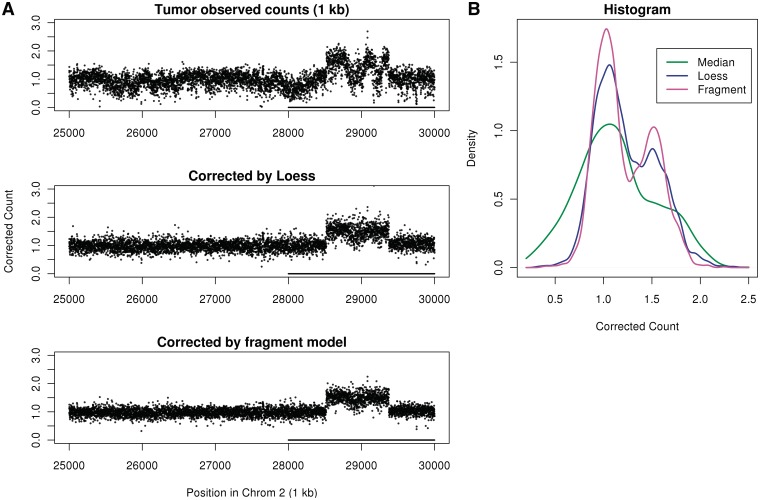
Figure 9.

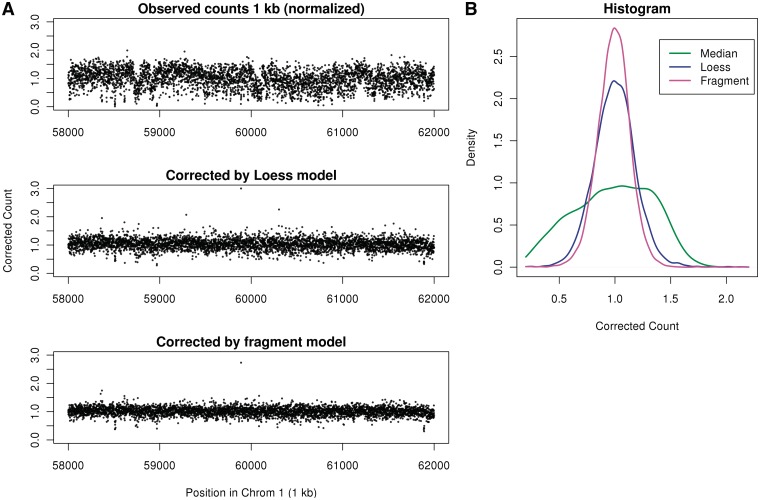
CN gain from tumor sample. Counts and corrected counts at position 29 000 kb on chromosome 2. (A) Unnormalized counts at 1 kb bins (top), corrected by loess (center) and corrected by fragment model (bottom). GC curves estimated on chromosome 1 (which has no large CN changes). (B) Histogram of normalized counts at 28–30 mb (underlined on left plots).

The choice of bin size should not matter much if the bias is linear. However, sampling a unimodal curve at the wrong scale will normally increase the variance. We therefore compared the absolute deviance from the curve at difference bin sizes (Table 2). The predictions were aggregated to 10 kb (regardless of estimation bin size). The results improve as bin size decreases. This is true, for both libraries, until we approach bin sizes of the order of the fragment length (300 bp for library 2, 175 bp for library 1). Counts of library 2 were scaled by median fragment rate to match library 1.

Table 2.

Prediction error (MAD) of loess model for different resolutions

Loess bin size (kb)	10	5	2	1	0.5	0.2
Normal Lib1	49.1	47.8	45.1	43.4	43.4	52.2
Normal Lib2	54.8	52.0	47.5	45.7	49.7	87.7

Error measured by mean absolute deviation around the predicted rates. The best predictions (minimal error) for each library are in bold. Rates were estimated using loess at the specified resolution, and then predictions were aggregated into 10 kb bins.

Indeed, we cannot expect reducing bin sizes to work for such small scales. On scales comparable to fragment sizes the bin-edge effects become substantial. Each of the different models for the GC effect (fragmentation, reads or full fragments) should imply a different correction strategy. Moreover, small bins have few reads / fragments, and so measuring variability around the mean becomes harder. Instead of binning, single position models (Figure 1) are introduced to measure GC effects in these smaller scales.

Single position models

Single position models allow us to compare different possible GC windows, estimate the effects for each and compare their TV scores. First we compare TV scores of GC windows starting at the 5′-end (a = 0) of a location (but having different lengths). We would expect to see the strongest effect either after a few bp (fragmentation effect), after 30–75 bp (read effect) or at the fragment lengths (full-fragment effect).

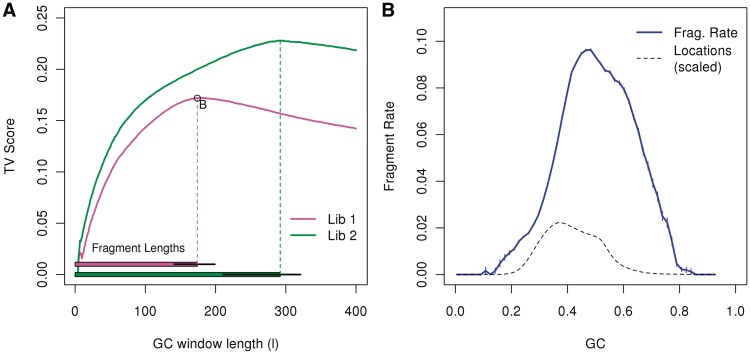
For both libraries, the full-fragment model achieves the highest TV score. In Figure 3A, the two curves represent TV scores of the two libraries from the normal sample. The horizontal bars on the bottom mark the median (and 0.05, 0.95 quantile) fragment sizes for the two libraries. TV scores for both libraries increase as the window size increases, with the strongest effects for windows almost matching the median fragment length: strongest effect for window of length 180 (W_0,180) for library 1 (median length=174), and length 295 (W_0,295) for library 2 (median length 293). For windows longer than that, the scores decrease.

Figure 3.

Single position models. (A) The top curves represent TV scores for GC windows of different lengths, all beginning at 0 (a = 0). The horizontal bars on the bottom mark the median fragment lengths (and 0.05, 0.95 quantiles). For each library, the strongest GC windows are those that encompass the full fragment. For library 1, we mark the optimal model (W_0,180), and show its resulting GC curve on the right panel (B). (We actually show W_2,176, removing 2 bp from each side of the fragment.) The GC curve measures the fragment rate given the fraction of GC in the window. Vertical lines (blue) represent 1 SD. For comparison, we plot the distribution of GC (dotted line) in our sample from chromosome 1 (scaled).

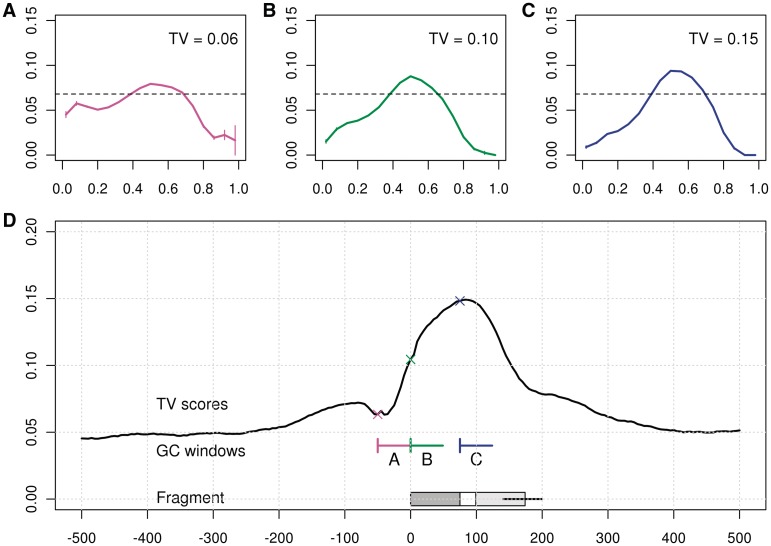
The GC curve that is estimated from the window W_2,176 is extremely sharp (Figure 3B) (this is W_0,180 after removing 2 bp on each end). In fact, strong unimodality can be seen on even smaller scales. Smaller windows (l = 50 bp) allow us to contrast a GC window that overlaps the read with a GC window that does not (W_0,50 versus W_75,50). (Figure 4B and C). The GC effect estimated from both windows has a unimodal shape, but the curve of the window overlapping the read is not as sharp as that of the window from the fragment center. If read composition were driving the GC effect, we would expect the first window to generate the sharper curve. That this is not the case, may imply that the GC effect is not driven by base calling or sequencing effects, but by the composition of the full fragment. (Rather, the sharper curves in the center imply a second weak bias near fragment ends, see below.) In contrast, Figure 4A shows the GC curve estimated from the 50 bp located just outside the fragment (W_− 50,50.) The curve is not unimodal, and has a noticeably lower TV score.

Figure 4.

Different lags. (A) GC curve of the window before the fragment, W_−50,50; (B) within the read, W_0,50 and (C) in the fragment center, not overlapping the read, W_75,50. (D) A plot of TV scores for 50 bp sliding windows (W_a,50). The x-axis marks a, the location of the window 5′-end relative to 5′-end of the fragment. On the bottom, we mark a fragment and its reads in relation to the GC windows from the top panels.

To further illuminate this (Figure 4D), we compute TV scores for other 50 bp GC windows with different lags. The TV curve traces the shape of the fragments: it ascends sharply for windows completely within the fragment, and then dips considerably for windows outside the 3′-end. The line is mostly symmetric around half the median-fragment length, decreasing as the windows extend over the 3′-ends of fragments. In fact, enumerating over many positions a and lengths l, the strongest windows are those overlapping most of the fragment but excluding the fragment ends. (Note that the 5′-end is perfectly aligned, the 3′ is not, due to varying fragment lengths.) The TV scores decay outside the fragment, but still reflect some GC dependence due to large-scale correlations in GC composition.

In Supplementary Figure S2, we contrast the TV plots generated from the forward strand with TV plots of the reverse strand. While the reads have exactly the same location (no matter the strand), the forward strand fragments extend to the 3′-end of the read whereas reverse strand fragments extend to the 5′-end. The TV score lines trace these shapes. After the proper inversion and shift, both GC curves estimated on the reverse strand and their TV scores match those from the forward strand.

Effect of fragment length

Within a library, we find that the length of fragments influences the shape of the GC curve. If GC depends on fragments and not reads, the GC is a quotient of two fragment parameters: the number of G and C bases, and the length of the fragment. We might expect the two parameters to interact to determine the rate of fragments. This is indeed the case. Within a single library, GC curves estimated on longer fragments peak at higher GC's.

Figure 5A displays a surface describing fragment rates for all (GC, length) pairs. We use the GC count of the full fragment excluding the first 2 bp on each end, corresponding to . Each horizontal cut of this surface represents a GC curve for fragments of a specific length.

Models restricted to long fragments (top of Figure 5A) tend to reach highest rates at higher GC counts (right). The shift toward high GC in longer curves persists in the rescaled curves (Figure 5B). The curves displayed here are represented by the dotted lines on (Figure 5A), but this time rescaled so that the x-axis is the fraction GC, not the count. We have seen similar patterns of GC length interactions in other data sets from different sequencing centers, though not all.

Local biases near fragment ends

While the unimodal effect is the strongest inhomogeneity in coverage, it is not the only one. We will discuss two (perhaps partially related) effects that are found near the fragment ends, and argue they are not driving the GC effects at larger bin sizes.

The first of these is a preference of AT near the fragment ends. Note that the GC curve based on a window just 5′ to the fragment (Figure 4A) reveals a second mode of AT-rich windows (in addition to the mode at 0.5 GC). Traces of this mode can also be seen in Figure 4B overlapping the read. The TV score when stratifying by this window are indeed lower (compared with the center of the fragment), reflecting the conflicting effects. This phenomena is strongest for 20–30 bp surrounding both the 5′ and 3′-end.

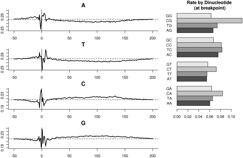
A second bias is in the composition of the few base pair around the fragment ends. It has been described before in RNA-seq (9). The relative frequency of nucleotides follows a position-specific pattern roughly starting four bases before fragment and ending 8–9 bases inside it (Figure 6, Left). We call this the ‘fragmentation effect’. Note that G and C are differently preferred, and so is A compared with T. Complementary effects can be seen on the 3′-end of the fragment, for a fixed fragment size. The fragment GC effect described before can also be seen—the small preference of G and C between 20 and 200 (reflecting fragment sizes). Rates stratified by dinucleotide counts are significantly different than singletons. In particular, the dinucleotide on which fragment rates depend the most is the pair surrounding the fragment end (the breakpoint), shown on the right. Fragments are much more likely to start within a CpG dinucleotide, than any other dinucleotide.

Figure 6.

Fragmentation effect. Left: relative abundance of nucleotides at fixed positions relative to fragment 5′-end. A horizontal dotted line marks the relative abundance of the base at mappable positions. Right: fragment rates when stratifying by the dinucleotide (−1,0). Dinucleotide counts overlapping the fragment 5′-end.

Aggregating effects and corrections

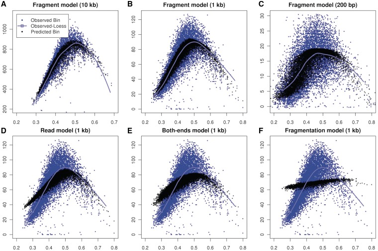
Local effects captured by the fragment model drive the GC curves found at larger scales. In Figure 7, Panels (A)–(C) compare GC to predicted and observed bin counts at various bin sizes. For all three bin sizes, the predicted counts (black) trace the observed loess line (blue), and also capture some of the variability around the curve.

Figure 7.

Aggregation of single location estimates. (A–C) Estimates based on the fragment GC curve (black) trace similar paths as loess (cyan) estimated on observed counts (blue) on multiple scales. (D–F) Estimates based on alternative models compared with observed counts on 1 kb bins. (D) Read model, predictions based on GC of the 5′ read only (W_0,75); (E) Two-ended model uses GC (30 bp) from both ends of the fragments; (F) Fragmentation model based on location-specific composition around the 5′-end. See Supplementary methods for details on how models for (E) and (F) were defined and estimated.

In contrast, models based on smaller portion of the fragment do not trace the observed curves. Figure 7D shows the estimates from the read (W_0,75). The predictions are too high for GC rich or GC-poor bins, and too low for intermediate GC bins. Similarly, the ‘two end model’ (Figure 7E), using GC (30 bp) from both ends of the fragment, produces unimodal predictions which are not sharp enough to capture the observed shape. Prediction based on the ‘fragmentation model’ (Figure 7F) does not produce sharp contrasts or unimodality. The methods of correction used for (Figure 7E) and (F) are described in detail in Supplementary data.

Correction based on the fragment and fragment-length models remove most GC-dependent fragment count variation. Predicted counts based on the fragment model are more accurate than predictions from the optimal loess model (MAD = 9.5 for fragment model, compared with 10.8 for loess model on 1 kb bins). The same holds for all bin sizes. Adding fragment-length into this model slightly improves the prediction quality (MAD = 9.1). Since adding length did not change the results greatly, we use the more parsimonious model for the rest of this work.

We visualize the correction in a region of chromosome 1 which has no CN changes. In Figure 8A uncorrected (but scaled) 1 kb bin counts display large low-frequency variations, which can be mistaken for CN events. The fragment model removes these variations better than the loess model. In Figure 8B, a histogram of corrected counts shows that the fragment correction produces tighter distribution of scaled counts around 1 compared with the loess model.

Figure 8.

Corrected counts of normal sample. (A) Counts in 1 kb bins not corrected for GC (top), corrected by loess (center) and corrected by fragment model (bottom), positions 58 000–62 000 kb of chromosome 1 (chr1). (B) Histograms of the corrected counts (random sample of 1 kb bins in chr1). Each point represents counts from both libraries (forward strand).

A similar correction on the tumor data reveals a hidden CN (both libraries, forward strand) in Figure 9. GC curves (for both the loess and fragment models) were estimated from chromosome 1, and corrected counts for a CN gain on chromosome 2 are shown. The CN gain is hidden in the uncorrected data due to low-frequency count variation driven by GC content. Both the fragment model correction and the loess correction reveal the CN gain. The fragment correction provides better separation between bands [see histograms in (Figure 9B)]. Also, it successfully corrects for different binning resolutions (Supplementary Figure S3). Note that chromosome 1 was used for GC estimation because it does not seem to have large CN changes (as seen in Figure 2).

Poisson and other variation

The estimated GC effect and mappability explain most the variation in the fragment coverage of the normal genome (though not all of it). In Table 3, we compute the RV after removing the GC effect in 1 kb bins. The GC model removes most of the variability in the binned counts, much more so than corrections based only on mappability. The RV of the fragment model is considerably smaller than that of the loess model. It is still larger than Poisson, though small areas with extremely high coverage cause most of this extra variance.

Table 3.

Residual variance (RV) from different models

Method	Total	MR	GR	1-GR/MR	P	GR/P
Loess	909	464	177	0.61	59	3
Fragment	909	464	137	0.7	59	2.33

Residual variance of GC models (GR) compared to RV from mappability model (MR) and to the expected variance of a heterogenous Poisson (P). Also displayed are the proportion of RV (after mappability correction) explained by GC (1−GR/MR); and the ratio between GC residuals and the expected Poisson variance (GR/P). Computed on 1 kb bins from normal sample (forward strand, library 1), after removing outlier bins.

For a comparison more robust to these high-coverage regions, we compare quantiles rather than variances. In Figure 10, we compare the 0.1 and 0.9 quantiles of observed counts grouped by the estimated fragment rates of different models (see ‘Material and Methods’ section). The variation in bins with very low observed counts is largely explained by mappability. However, mappability cannot explain variation of higher counts, and the spread between the quantiles is approximately double that of the Poisson. Models taking GC content into account produce much tighter spreads. The fragment-length model (the green curve) consistently leaves less variation around the estimated rates than the loess model (blue).

Figure 10.

Comparison to Poisson variation. 0.1 and 0.9 quantiles of observed counts grouped by estimated rates. Models that predict better will have narrower vertical spreads. Variation around the mean of the fragment model (green), the loess (blue) and mappability (black) are compared to variation around a Poisson (red).

Additional data sets

In the above analysis, we described a single tumor–normal pair produced by a single lab, but our results are general to many examined samples from multiple labs. In Figure 11, we show four descriptive plots from a different data set (based on HCC1569 cell line, see Table 1 for details). The GC has a strong effect on fragment counts, and this relation is unimodal (Figure 11A). The highest TV score is for a window of approximately fragment length (Figure 11B), resulting in a sharp GC curve (shown in Figure 11C) which predict the GC trends (Figure 11D). A distinct difference is the lack of length dependence of the fragments (data not shown). The AT preference near fragment ends is also missing, further proving that it is not the major source of the GC bias. Two additional sets of data are shown in the Supplementary Data.

DISCUSSION

Large biases in fragment counts related to the GC composition of regions were found in the data sets we examined. These observed effects have a recurring unimodal shape, but varied considerably between different samples.

We have shown that this GC effect is mostly driven by the GC composition of the full fragment. Conditioning on the GC of the fragments captures the strongest bias, and removing this effect provides the best correction, compared with alternative GC windows. When single base pair predictions based on the fragment composition are aggregated, the results trace the observed GC dependence. This cannot be said about local effects that take only the reads into account. This conclusion holds for various data sets, with different fragment length composition, read lengths and GC effect shapes.

That the GC curve is unimodal is key to this analysis. In all data sets shown, the rate of GC-poor or GC-rich fragments is significantly lower than average, in many cases zero. Unimodality was overlooked by Dohm et al. (1), probably because GC-rich areas are rare (especially in simpler organisms). Even in humans, it is hard to spot this effect if counts are binned by GC quantiles instead of GC values. Nevertheless, it is this departure from linearity that allowed pinpointing an optimal scale—the fragment size. In that, unimodality gives us important clues as to the causes of the GC bias.

While we have described other sequence-related biases, we believe they are not driving the strong coverage GC biases. These include an increased coverage when the ends are AT rich, and location-specific fragmentation biases near the fragment ends. We have shown that the end effects, as measured on the 5′-end, are far weaker than the effect from the full fragment. They are also surprisingly negligible in the context of larger bins. Still, they might locally mitigate the fragment GC effect: the effect of fragment length on GC curve seems to be associated with these biases.

Our conclusions seem to complement those of Aird et al. (12). If PCR is the major source of the GC bias, we would expect GC of the full fragment to be associated with the bias, rather than the GC of one or both reads. We have shown this is indeed the case. Moreover, data sets generated according to a PCR-free protocol (10) and an optimized PCR protocol (12) both display a reduced GC bias (Supplementary Figure S4 and S5). It should be noted that even these optimized PCR protocols can still display significant biases and may require GC correction.

Our refined description of the GC effect is of practical value for GC correction. First of all, the non-linearity of the GC effect is a warning sign regarding two-sample correction methods. In the main example we study, the pair of normal and tumor samples do not have the same GC curves. We have seen this in additional data sets as well. Using normal counts to correct tumor counts could sometimes produce GC-related artifacts, which might lead to faulty segmentations. The GC effects of samples should be carefully studied before such corrections are made.

A single sample correction for GC requires a model, and we demonstrate the importance of choosing the best model. Overlapping windows smaller than the fragment fail to remove the bulk of the GC effect. Similarly, using read coverage rather than fragment count hurts the correction. Instead, measuring fragment rate for single base pair positions, decouples the GC modeling from the downstream analysis. Thus, it removes the lower threshold on the scale of analysis, providing single base pair estimates, which can be later smoothed by the researcher as needed (or binned into uneven bins if needed). An important benefit of DNA-seq over previous technologies is that simply repeating the experiment can increase the resolution of the analysis. Our model assures that this increased resolution does not hurt the GC correction.

Unlike other bias correction methods, such as BEADS (14), we generate weights (predicted fragment rates) for the genomic location rather than for the observed reads. Mappable genomic positions are stratified according to the GC of a hypothetical fragment, and rates per GC stratum are estimated by counting the fragments at those same positions. Estimating predicted rates for both covered and uncovered locations can help detect deletions, and these predicted rates form a natural input for downstream analysis using heterogeneous Poisson models. Another important novelty is the use of TV scores to determine the representative ‘fragment length’ of each data set, one that best fits the distribution of fragment lengths and properly discards the fragment end biases. This procedure can be critical when length information is unavailable (i.e. for single-ended reads). A more detailed comparison to BEADS is found in the Supplementary Figures S9 and S10.

In this work, we estimated DNA abundance from non-tumor genomes, implicitly assuming that abundance of DNA along the genome is uniform. It is true that CN variation may occur in non-tumor sequences; these jumps are rare however, and by random sampling we hope to average over any large CN changes. That the windows are small should reduce the dependence between GC and specific positions in the genome. From our experience, estimating GC curves using small windows turned out to be surprisingly robust to CN changes on tumor data (as displayed above). To extend this method to other applications or protocols would require identifying regions in which the signal of interest is not expected to vary, and perhaps co-estimation of the abundance and the GC effect. That said, for CN purposes there is enough data to get stable estimates of the GC effect.

Our prediction accounts for a large portion of the variation, but residual variation is still present. Additional inhomogeneities in fragment rates include unexplained hot spots or zero-counts, as well as milder low and high frequency variation in the counts. The first two categories may be due to errors in the annotation of the genome or amplification artifacts. The latter point to existence of additional factors that affect fragment rates, which is to be expected. We have discussed additional sequenced-related biases, including fragmentation and AT preference. The tools developed here, primarily the total variation scores, allow analysts to further investigate these effects as needed. Nevertheless, by and large, our model successfully describes the bulk of the low-frequency variability, which confounds segmentation to CN regions.

One effect that we have not deeply explored is the relation between sequencing error probability and the GC effect. In the Supplumentary Data, we have shown evidence that the global GC of the fragment can effect the sequencing error probability. Especially for longer reads, changing the parameterization of the mapping processes can sometimes produce different mappability patterns related to the GC composition. There have been reports (11) that specific sequences in reads are more prone for errors, for example a GGC sequence. A better model for reads that are harder to sequence would allow better estimation of the fragment GC effect in the GC-rich regions, and improve the accuracy of the corrections. Jointly correcting by the GC of the read as well as the GC of the fragment may be a useful approximation for this effect.

Our analysis focused only on DNA-seq data from human subjects, but results from this work can be extended. GC content biases were seen in additional experimental protocols using high-throughput sequencing. [See Supplementary Figures S7 and S8, and Ref. (14) for similar correction approaches in ChIP-seq data.] Some of these protocols focus on highly localized signals on the genome, and could also benefit from strand-specific and uneven bin normalization. Moreover, when length of the fragments is constrained (exon sequencing, RNA-seq), a model taking both GC and fragment length into account may prove important. Fitting the model for each application is a challenge; still we believe that all these applications can benefit from our refined GC model.

SUPPLEMENTARY DATA

Supplementary Data are available at NAR Online: Supplementary Figures S1–S10, Supplementary Methods and Supplementary References (10,12,14,21).

FUNDING

National Institutes of Health (grant number 3U24CA143799-02S1 to Y.B.). National Science Foundation VIGRE Graduate Fellowship. National Institutes of Health (grant number 5R01 GM083084-03 to T.P.S.). Funding for open access charge: National Institutes of Health (grant 5R01 GM083084-03).

Conflict of interest statement. None declared.

REFERENCES

- 1.Dohm JC, Lottaz C, Borodina T, Himmelbauer H. Substantial biases in ultra-short read data sets from high-throughput DNA sequencing. Nucleic Acids Res. 2008;36:e105. doi: 10.1093/nar/gkn425. [DOI] [PMC free article] [PubMed] [Google Scholar]
- 2.Chiang DY, Getz G, Jaffe DB, O'Kelly MJ, Zhao X, Carter SL, Russ C, Nusbaum C, Meyerson M, Lander ES. High-resolution mapping of copy-number alterations with massively parallel sequencing. Nat. Methods. 2008;6:99–103. doi: 10.1038/nmeth.1276. [DOI] [PMC free article] [PubMed] [Google Scholar]
- 3.Quail MA, Kozarewa I, Smith F, Scally A, Stephens PJ, Durbin R, Swerdlow H, Turner DJ. A large genome center's improvements to the Illumina sequencing system. Nat. Methods. 2008;5:1005–1010. doi: 10.1038/nmeth.1270. [DOI] [PMC free article] [PubMed] [Google Scholar]
- 4.Ivakhno S, Royce T, Cox AJ, Evers DJ, Cheetham RK, Tavaré S. CNAseg—a novel framework for identification of copy number changes in cancer from second-generation sequencing data. Bioinformatics. 2010;26:3051. doi: 10.1093/bioinformatics/btq587. [DOI] [PubMed] [Google Scholar]
- 5.Yoon S, Xuan Z, Makarov V, Ye K, Sebat J. Sensitive and accurate detection of copy number variants using read depth of coverage. Genome Res. 2009;19:1586. doi: 10.1101/gr.092981.109. [DOI] [PMC free article] [PubMed] [Google Scholar]
- 6.Boeva V, Zinovyev A, Bleakley K, Vert JP, Janoueix-Lerosey I, Delattre O, Barillot E. Control-free calling of copy number alterations in deep-sequencing data using GC-content normalization. Bioinformatics. 2011;27:268. doi: 10.1093/bioinformatics/btq635. [DOI] [PMC free article] [PubMed] [Google Scholar]
- 7.Miller CA, Hampton O, Coarfa C, Milosavljevic A. ReadDepth: a Parallel R Package for detecting copy number alterations from short sequencing reads. PLoS One. 2011;6:e16327. doi: 10.1371/journal.pone.0016327. [DOI] [PMC free article] [PubMed] [Google Scholar]
- 8.Teytelman L, Özaydn B, Zill O, Lefrançois P, Snyder M, Rine J, Eisen MB. Impact of chromatin structures on DNA processing for genomic analyses. PLoS One. 2009;4:e6700. doi: 10.1371/journal.pone.0006700. [DOI] [PMC free article] [PubMed] [Google Scholar]
- 9.Hansen KD, Brenner SE, Dudoit S. Biases in Illumina transcriptome sequencing caused by random hexamer priming. Nucleic Acids Res. 2010;38:e131. doi: 10.1093/nar/gkq224. [DOI] [PMC free article] [PubMed] [Google Scholar]
- 10.Kozarewa I, Ning Z, Quail MA, Sanders MJ, Berriman M, Turner DJ. Amplification-free Illumina sequencing-library preparation facilitates improved mapping and assembly of (G+C)-biased genomes. Nat. Methods. 2009;6:291–295. doi: 10.1038/nmeth.1311. [DOI] [PMC free article] [PubMed] [Google Scholar]
- 11.Nakamura K, Oshima T, Morimoto T, Ikeda S, Yoshikawa H, Shiwa Y, Ishikawa S, Linak MC, Hirai A, Takahashi H, et al. Sequence-specific error profile of Illumina sequencers. Nucleic Acids Res. 2011;39:e90. doi: 10.1093/nar/gkr344. [DOI] [PMC free article] [PubMed] [Google Scholar]
- 12.Aird D, Ross MG, Chen WS, Danielsson M, Fennell T, Russ C, Jaffe DB, Nusbaum C, Gnirke A. Analyzing and minimizing PCR amplification bias in Illumina sequencing libraries. Genome Biol. 2011;12:R18. doi: 10.1186/gb-2011-12-2-r18. [DOI] [PMC free article] [PubMed] [Google Scholar]
- 13.Bravo HC, Irizarry RA. Model-based quality assessment and base-calling for second-generation sequencing data. Biometrics. 2010;66:665–674. doi: 10.1111/j.1541-0420.2009.01353.x. [DOI] [PMC free article] [PubMed] [Google Scholar]
- 14.Cheung M, Down TA, Latorre I, Ahringer J. Systematic bias in high-throughput sequencing data and its correction by BEADS. Nucleic Acids Res. 2011;39:e103. doi: 10.1093/nar/gkr425. [DOI] [PMC free article] [PubMed] [Google Scholar]
- 15.Li H, Durbin R. Fast and accurate short read alignment with Burrows–Wheeler transform. Bioinformatics. 2009;25:1754. doi: 10.1093/bioinformatics/btp324. [DOI] [PMC free article] [PubMed] [Google Scholar]
- 16.Kuan PF, Chung D, Pan G, Thomson JA, Stewart R, Keles S. A statistical framework for the analysis of ChIP-Seq data. J. Am. Stat. Assoc. 2011;106:891–903. doi: 10.1198/jasa.2011.ap09706. [DOI] [PMC free article] [PubMed] [Google Scholar]
- 17.Langmead B, Trapnell C, Pop M, Salzberg SL. Ultrafast and memory-efficient alignment of short DNA sequences to the human genome. Genome Biol. 2009;10:R25. doi: 10.1186/gb-2009-10-3-r25. [DOI] [PMC free article] [PubMed] [Google Scholar]
- 18. R-Development-Core-Team (2010) R: A Language and Environment for Statistical Computing, R Foundation for Statistical Computing. Vienna, Austria. [Google Scholar]
- 19.Durrett R. Probability: Theory and Examples. Cambridge University Press, Cambridge, UK; 2010. [Google Scholar]
- 20.Bentley DR, Balasubramanian S, Swerdlow HP, Smith GP, Milton J, Brown CG, Hall KP, Evers DJ, Barnes CL, Bignell HR, et al. Accurate whole human genome sequencing using reversible terminator chemistry. Nature. 2008;456:53–59. doi: 10.1038/nature07517. [DOI] [PMC free article] [PubMed] [Google Scholar]
- 21.Li H, Ruan J, Durbin R. Mapping short DNA sequencing reads and calling variants using mapping quality scores. Genome Res. 2008;18:1851–1858. doi: 10.1101/gr.078212.108. [DOI] [PMC free article] [PubMed] [Google Scholar]
Associated Data
This section collects any data citations, data availability statements, or supplementary materials included in this article.