Imaging neuroscience: Principles or maps?

Abstract

This article reviews some recent trends in imaging neuroscience. A distinction is made between making maps of functional responses in the brain and discerning the rules or principles that underlie their organization. After considering developments in the characterization of brain imaging data, several examples are presented that highlight the context-sensitive nature of neuronal responses that we measure. These contexts can be endogenous and physiological, reflecting the fact that each cortical area, or neuronal population, expresses its dynamics in the context of interactions with other areas. Conversely, these contexts can be experimental or psychological and can have a profound effect on the regional effects elicited. In this review we consider experimental designs and analytic strategies that go beyond cognitive subtraction and speculate on how functional imaging can be used to address both the details and principles underlying functional integration and specialization in the brain.

An imaging neuroscientist who wants to understand some of the organizational principles that underlie brain function is faced with a great challenge: Imagine that we took you to a forest and told you, “Tell us how this forest works. Many scientists are interested in this forest and study it using a variety of techniques. Some study a particular species of flora or fauna, some its geography. You won’t have time to talk to them all but you can read what they write in specialist journals. We should warn you however that many have specific interests and tend to study only the accessible parts of the forest.” You accept the challenge, and, to make things interesting, we place two restrictions on you. First, you can only measure one thing. Second, although you can make measurements anywhere, you can only take them at weekly intervals. This problem is not unlike that facing neuroimaging. Of all the diverse aspects of neuronal dynamics, imaging is only sensitive to hemodynamic responses (a distal measure of neuronal activity), and these measurements can only be made sparsely in time. Faced with the forest problem one would acquire data, generating map after map of the measured variable. One might try to make some inferences about regional differences and try to understand the changes measured, initially at any one point and then in the context of changes elsewhere. These measures might be related to meteorological changes, seasonal variations, and so on. In short, one would make maps and then try to characterize their dynamical behavior. What, however, is the primary objective? Is it the construction of detailed maps or is it the interpretation of their dynamics in terms of simple rules or principles that govern them. We suggest that both aspects are crucial and develop this argument further in relation to recent trends in functional neuroimaging. This article is divided into four sections. In the first we review some of the general motivations behind imaging neuroscience in terms of the distinction between making maps of functional anatomy and the principles that emerge from them. In the second section we review the way in which the models or tools used to analyze data are likely to develop. In the third and fourth sections we introduce some specific examples relating to functional integration and the different sorts of regionally specific brain responses that can be characterized.

Principles or Maps?

Functional maps in neuroimaging rely on identifying areas that respond selectively to various aspects of cognitive and sensorimotor processing. These maps are likely to become successively more refined: On the one hand they will contain more detail as the resolution of the techniques employed increases. The spatial resolution of functional magnetic resonance imaging (fMRI) is already sufficient to discern structures like the thick, thin, and interstripe organization within V2. Temporal resolution is in the order of seconds and can be supplemented with magneto- or electrophysiological information at a millisecond level. The second sort of refinement may be in terms of the taxonomy of regionally specific effects themselves: Neuroimaging, to date, largely has focused on “activations.” However, regionally specific effects not only conform to a taxonomy based on anatomy (i.e., which anatomical area is implicated) but also in relation to the nature of the effect. An example of this is the distinction between regionally specific “activations” and regionally specific “interactions” (i.e., context-sensitive activations observed in factorial experiments) (1). A further extension of “mapping” is into the domain of interactions or connections among areas. Although prevalent in the context of anatomical connectivity (2), maps of functional or effective connections have yet to be established. The latter are likely to be more complicated than their anatomical equivalents by virtue of their dynamic and context-sensitive nature (see below).

Map making per se is not the only aspect of imaging neuroscience. Understanding the principles or invariant features of these maps, and their associated mechanisms, is an important aim. There is a distinction between identifying an interaction, e.g., between two extrastriate areas, and the principles that pertain to all such interactions. For example, there is a difference between demonstrating a modulatory influence of posterior parietal complex on V5 (the human homologue of primate area MT) and the general principle that backward projections, from higher-order areas, are more modulatory than their forward counterparts. Note, however, that this principle would depend on fully characterizing all the interactions among extrastriate areas. This reiterates the importance of cartography, in this instance, a cartography of connections. Another example of principles that derive from empirical observations can be taken from the work of complexity theorists, wherein certain degrees of “connectivity” at the level of gene–gene interactions give rise to complex dynamics (3). This principle of sparse connectivity has emerged again in relation to the complexity of neuronal interactions (4). What are the sorts of principles that one is looking for in imaging neuroscience? The “principle of functional specialization” is now well established and endorsed by human neuroimaging studies. If we define functional specialization in terms of anatomically specific responses that are sensitive to the context in which these responses are evoked, then, by analogy, “functional integration” can be thought of as anatomically specific interactions between neuronal populations that are similarly context-sensitive. In a sense, functional integration is a principle, but it is not very useful. Examples of more useful principles might include a principle of sparse connectivity (e.g., functional integration is mediated by sparse extrinsic connections that preserve specialization within systems that have dense intrinsic connections) or that, in relation to forward connections, backward connections are modulatory. In summary, a detailed empiricism is a prerequisite for the emergence of organizational principles. For some neuroscientists the principles themselves might be the ultimate goal, but these principles will only be derived from maps of the brain. For others, relating the maps to cognitive architectures and psychological models may be the ultimate goal, but this in itself requires a principled approach.

Models or Tools?

In this section we consider the status of various models that are used to analyze or characterize brain function and how they are likely to develop. The models one usually comes across in neuroscience are of three types. First, there are biologically plausible neural network or synthetic neural models (5). Second are the mathematical models employed in linear and nonlinear system identification, and third are the statistical models used to characterize empirical data (6). This section suggests that the increasing sophistication of statistical models will render them indistinguishable from those used to identify the underlying system. Similarly, synthetic neural models that are currently used to emulate brain systems and study their emergent properties will lend themselves to reformulations in terms of those required for system identification. The importance of this is that (i) the parameters of synthetic neural models, for example, the connection parameters and time constants, can be estimated directly from empirical observations and (ii) the validity of statistical models, in relation to what is being modeled, will increase. Another way of looking at the distinctions between the various sorts of models (and how these distinctions might be removed) is to consider that we use models either to emulate a system, or to define the nature or form of an observed system. When used in the latter context, the empirical data are used to determine the exact parameters of the specified model where, in statistical models, inferences can be made about the parameter estimates. In what follows we will review statistical models and how they may develop in the future and then turn to an example of how one can derive a statistical model from one normally associated with a nonlinear system identification. The importance of this example is that it shows how a model can be used, not only as a statistical tool, but as a device to emulate the behavior of the brain under a variety of circumstances.

Linear Models.

The most prevalent model in imaging neuroscience is the general linear model. This simply expresses the response variable (e.g., hemodynamic response) in terms of a linear sum of explanatory variables or effects in a “design matrix.” Inferences about the contribution of these explanatory variables are made in terms of the parameter estimates, or coefficients, estimated by using the data. There are a number of ways in which one can see the general linear model being developed in neuroimaging; for example, the development of random- and mixed-effect models that allow one to generalize inferences beyond the particular group of subjects studied to the population from which the subjects came, or the increasingly sophisticated modeling of evoked responses in terms of wavelet decomposition. Here we will focus on two examples: (i) model selection and (ii) inferences about multiple effects using statistical parametric maps of the F statistic [SPM(F)].

Generally, when using statistical models, one has to choose from among a hierarchy of models that embody more and more effects. Some of these effects may or may not be present in the data, and the question is, “which is the most appropriate model?” One way to address this question is to see whether adding extra effects significantly reduces the error variance. When the fit is not significantly improved one can cease elaborating the model. This principled approached to model selection is well established in other fields and will probably prove useful in neuroimaging. One important application of model selection is in the context of parametric designs and characterizing evoked hemodynamic responses in fMRI. In parametric designs it is often the case that some high-order polynomial “expansion” of the interesting variable (7) (e.g., the rate or duration of stimulus presentation) is used to characterize a nonlinear relationship between the hemodynamic response and this variable. Similarly, in modeling evoked responses in fMRI, the use of expansions in terms of temporal basis functions has proved useful (8). These two examples have something in common. They both have an “order” that has to be specified. The order of the polynomial regression approach is the number of high-order terms employed, and the order of the temporal basis function expansion is the number of the basis functions used. Model selection has a role here in determining the most appropriate or best model order.

Models that use expansions bring us to the second example. Recall that in general the contribution of designed effects is reflected in the parameter estimates of the coefficients relating to these effects. In the case of polynomial expansions or temporal basis functions these are the set of coefficients of the high-order terms or basis functions. Unlike simple activations (or effects corresponding to a particular linear combination of the parameter estimates), inferences based on these high-order models must be a collective inference about all of these coefficients together. This inference is made with the F statistic and speaks to the usefulness of the SPM(F) as an inferential tool. The next section presents an example of the SPM(F) in action and introduces models used in nonlinear system identification.

Nonlinear Models.

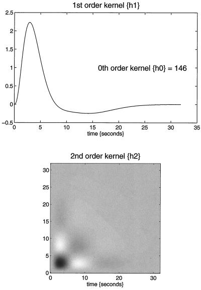
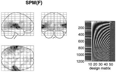
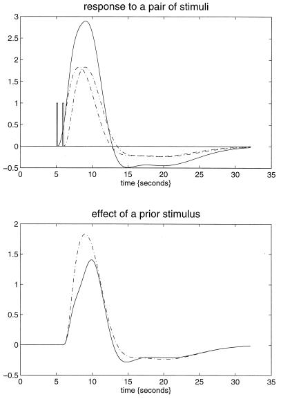
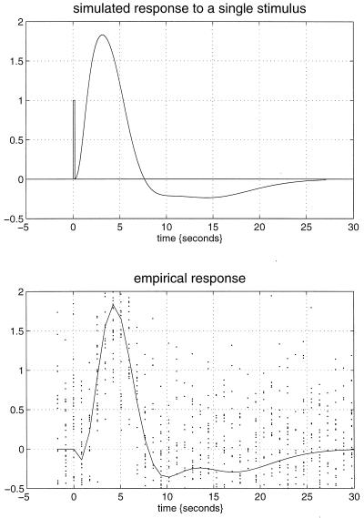
How can we best characterize the relationship between stimulus presentation and the evoked hemodynamic response in fMRI? Hitherto the normal approach has been to use a stimulus waveform that conforms to the presence or absence of a particular stimulus attribute, convolve (i.e., smooth) this with an estimate of the hemodynamic response function, and see if the result can predict what is observed. Our using an estimate of the hemodynamic response function assumes that we know the nature or form of this response and furthermore precludes nonlinear effects. A more comprehensive approach would be to use nonlinear system identification and pretend that the stimulus was the input and that the observed hemodynamic response was the output. This approach posits a very general form for the relationship and uses the observed inputs and outputs to determine the parameters of the model that optimize the match between the observed and predicted hemodynamic responses. The approach that we have adopted uses a Volterra series expansion (8). This expansion can be thought of as a nonlinear convolution and can be shown to emulate the behavior of any nonlinear, time-invariant dynamical system. The results of this analysis are a series of Volterra kernels of increasing order. The zero-order kernel is simply a constant, the first order kernel corresponds to the hemodynamic response function usually arrived at in linear analyses, and the second, and higher-order, kernels embody the nonlinear dependencies of response on stimulus input. By using a series of mathematical devices (second-order approximations and expansion of the coefficients in terms of temporal basis functions) we were able to reformulate the Volterra series in terms of the general linear model and use standard techniques to estimate and make statistical inferences about these kernels. An example of the kernel estimates for a voxel in periauditory cortex is shown in Fig. 1. This estimate was based on a parametric study of evoked responses to words presented at varying frequencies and is fairly typical of a nonlinear hemodynamic response function. The associated SPM(F), shown in a standard anatomical space, testing for the significance of the Volterra kernels is shown in Fig. 2. At this point we could conclude that evoked responses show a highly significant nonlinear response and present the characterization of this response in terms of the kernel coefficients (Fig. 1). However, we can go further and use the parameter estimates to specify a model that can be used to emulate responses to a whole range of auditory inputs. As an example, consider the response to a pair of words that are presented close together in time, as distinct from when they are presented in isolation. Fig. 3 demonstrates the results of this simulation and shows that the presence of a prior stimulus attenuates the response to a second. The key thing to note here is that we are performing “virtual” experiments on the model, presenting it with stimuli that were never actually used. Indeed, we can determine the model’s response to a single word. The results of this analysis are shown in Fig. 4 along with the empirically determined responses from a real experiment where single words were presented in isolation. In conclusion, the distinction between models that are used solely to confirm our predictions about observed brain responses may, in the future, become sufficiently unconstrained and general as to provide the basis for simulated experiments.

Figure 1.

Volterra kernels h⁰, h¹, and h² based on parameter estimates from a voxel in the left superior temporal gyrus at −56, −28, and 12 mm. These kernels can be thought of as a characterization of the second-order hemodynamic response function. The first-order kernel (Upper) represents the (first-order) component usually presented in linear analyses and reflects the contribution of the input as a function of time. The second-order kernel (Lower) is presented in image format and reflects the contribution of the product of the input at two distinct times in the recent past. The color scale is arbitrary; white is positive and black is negative.

Figure 2.

(Left) SPM(F) testing for the significance of the first- and second-order kernel coefficients (h¹ and h²) in a word-presentation rate, single-subject fMRI experiment. This is a maximum-intensity projection of a statistical process of the F statistic, after a multiple-regression analysis at each voxel. The format is standard and provides three orthogonal projections in the standard space conforming to that described in Talairach and Tournoux (14). The grey scale is arbitrary, and the SPM(F) has been thresholded (F = 32). (Right) The design matrix used in the analysis. The design matrix comprises the explanatory variables in the general linear model. It has one row for each of the 1,200 scans and one column for each explanatory variable or effect modeled. The left-hand columns contain the explanatory variables of interest, x_i(t) and x_i(t),x_j(t), where x_i(t) is word presentation rate convolved with the ith basis function used in the expansion of the kernels. The remaining columns contain covariates or effects of no interest designated as confounds. These include (left to right) a constant term (h⁰), periodic (discrete cosine set) functions of time to remove low-frequency artifacts and drifts, global or whole brain activity G(t), and interactions between global effects and those of interest, G(t).x_i(t) and G(t).x_i(t),x_j(t). The latter confounds remove effects that have no regional specificity.

Figure 3.

(Upper) The simulated responses to a pair of words (bars) (1 sec apart) presented together (solid line) and in isolation (broken lines) based on the second-order hemodynamic response function in Fig. 1. (Lower) The response to the second word when preceded by the first (broken line), obtained by subtracting the response to the first word from the response to both, and when presented alone (broken). The difference reflects the impact of the first word on the response to the second.

Figure 4.

(Upper) Hemodynamic response to a single word (bar at 0 sec) modeled by using the Volterra kernel estimates of Fig. 1. (Lower) The empirical event-related response in the same region based on an independent, event-related, single-subject fMRI experiment. The solid line is the fitted response using only first-order kernel estimates, and the dots represent the adjusted responses.

Functional Integration in the Brain

One overriding aspect of the brain is its connectedness, suggesting that the interactions and relationships between activity in different parts of the brain may be as important as regionally specific dynamics. Perhaps what we search for is a “functional architecture” as opposed to a “functional anatomy,” where the architecture embodies the interactions and integration that bridge between the dynamics of specialized areas. In what follows, we consider a number of developments in neuroimaging that relate to functional integration and effective connectivity among specialized areas.

Effective Connectivity.

Functional integration is usually inferred on the basis of correlations among measurements of neuronal activity. However, correlations can arise in a variety of ways. For example, in multiunit electrode recordings they can result from stimulus-locked transients evoked by a common input or reflect stimulus-induced oscillations mediated by synaptic connections. Integration within a distributed system is usually better understood in terms of “effective connectivity” as distinct from the correlations themselves. Effective connectivity refers explicitly to the influence that one neural system exerts over another (9), either at a synaptic (i.e., synaptic efficacy) or population level (10, 11). There are two important aspects of effective connectivity: (i) effective connectivity is dynamic, i.e., activity- and time-dependent, and (ii) it depends on a model of the interactions. To date, the models employed in functional neuroimaging have been inherently linear (12). There is a fundamental problem with linear models. They assume that the multiple inputs to a region are linearly separable and do not interact. This precludes dynamic or activity-dependent connections that are expressed in one sensorimotor or cognitive context and not in another. The resolution of this problem lies in adopting nonlinear models that include terms that model the interactions among inputs. These interactions can be construed as a context- or activity-dependent modulation of the influence that one region exerts over another. This is an important point, suggesting that second-order models represent the minimum order necessary for a proper characterization of context-sensitive interactions.

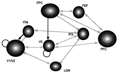
One approach to this characterization involves an extension of the above nonlinear model of hemodynamic responses that employed the Volterra series. In this instance, instead of considering the nonlinear response to a stimulus input, we replace the stimulus with activities measured in other parts of the brain. The Volterra kernels, which mediate the influences of distant regions, provide a comprehensive model of effective connectivity. These estimates are, as above, expressed in terms of kernel coefficients, and inferences can be made about their significance using standard statistical techniques. Although we will not go into details here, these sorts of analyses provide measurements of the direct and modulatory influences of one region on another and a P value associated with these effects. A typical example of the connectivity that is obtained from this sort analysis is shown in Fig. 5. This analysis was based on an fMRI study of visual motion. Subjects were presented with radially moving stimuli under different attentional conditions (see Fig. 5 legend). These results demonstrate the role of the posterior parietal cortex in modulating the effective connections to the motion-sensitive area, V5, that may mediate the attentional modulation of responses to its inputs. This attentional modulation represents a context-sensitive change in effective connections to V5.

Figure 5.

Effective connections associated with visual attention to motion. Direct effects (of one region on another) are shown in gray, and modulatory effects are shown in black. Direct effects pertain to terms that include only the activity of the source region. Modulatory effects were assessed by using the contribution of second-order terms that involve the source and another (modulated) input. Note that direct effects are almost always reciprocal and conform to predictions based on anatomical connectivity. Modulatory effects are limited to interactions between posterior parietal cortex (PPC) and V5 and between V3a and V1/V2. V1/V2 and V5 also intrinsically modulate their responses to afferent input. All the connections shown are significant at P < 0.05 (corrected for the number of connections tested). These effects were tested using the F statistic after a multiple regression for serially corrected data based on a Volterra series model of interregional influences. The modulatory interaction between PPC and V5 was extremely significant (F = 3.49, df = 25,691, P < 0.001, corrected).

Psychophysiological Interactions.

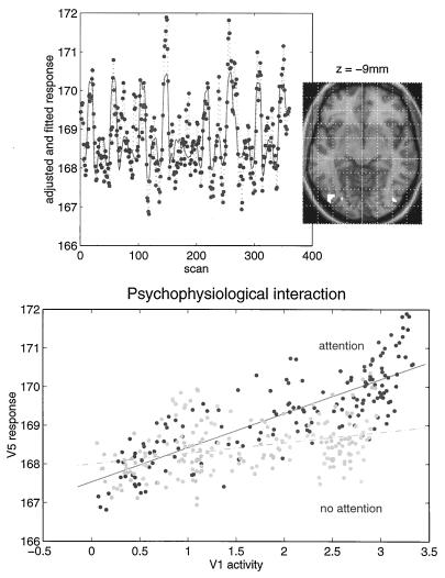
Modulation and context-sensitive changes in effective connectivity are important aspects of functional integration. Psychophysiological interactions refer to the interaction between some psychological or experimental context and physiological activity measured somewhere else in the brain. The idea here is to try and explain the responses observed, at one point in the brain, in terms of an interaction between the afferent input from another region and some designed, stimulus-specific, or cognitive variable. Generally, interactions are expressed in terms of the effect of one factor on the effect of another. Psychophysiological interactions therefore can be looked at from two points of view. First, a psychological or sensory factor can affect or modulate the physiological influence of one brain area on another. Second, the same interaction can be construed as a modulation of a target area’s responses to the sensory, or cognitive changes, by modulatory influences from the source area. The empirical example that we have chosen to illustrate this involves the fMRI study mentioned above of attention to visual motion. In this study, subjects were asked to view radially moving dots that gave the impression of “optic flow.” In between these stimuli the subject simply viewed a fixation point. On alternate presentations of the moving stimuli the subject was asked to attend to changes in the speed in the stimuli (these changes in speed did not actually occur). We were interested in whether attention could be shown to modulate the influence of V1/V2 complex on V5. We addressed this by regressing the activity at every voxel, on that in V1/V2, under the two attentional states separately. We tested the significance of the difference in the resulting regression slopes (i.e., the psychophysiological interaction between V1/V2 complex activity and attentional set) to give an SPM(t). Significant (P < 0.05, corrected) voxels are shown in white on a structural T₁-weighted MRI in Fig. 6 Upper and correspond to a region in the vicinity of V5. The Lower panel shows an example of the regression for the most significant voxel in this region and demonstrates that when subjects were expecting to detect changes in the motion of a visual stimulus, the regression slope was markedly steeper. In other words, the influence of V1/V2 on V5 was positively modulated by attention to this aspect of visual motion.

Figure 6.

(Upper) SPM thresholded at P = 0.001 (height uncorrected) and P = 0.05 (volume corrected) superimposed on a structural T₁-weighted image. This SPM tests for a significant psychophysiological interaction between activity in V1/V2 and attention to visual motion. The most significant effects are seen in the vicinity of V5 (white region, lower right). The time series of the most significant (Z = 4.46) voxel in this region is shown in the Upper panel (line, fitted data; dots, adjusted data). (Lower) Regression of V5 activity (at 42, −78, and −9 mm) on V1/V2 activity when the subject was asked to attend to changes in the speed of radially moving dots and when the subject was not asked to. The lines correspond to the regression. The dots correspond to the observed data adjusted for confounds other than the main effects of V1/V2 activity (dark grey dots, attention; light grey dots, no attention). Attention can be seen to augment the influence of V1/V2 on V5.

Let us look again at the two regression slopes in Fig. 6. Recall above that there are two interpretations of psychophysiological reactions: (i) a context-specific change in the influence or connectivity between two regions or (ii) a modulation of responsiveness by this influence. The first interpretation is more natural in this context, in the sense that attention can be thought of as modulating the influences that V1/V2 exerts over V5. However, the complementary perspective is equally valid. In this instance, attention-dependent responses in V5 are realized only in the presence of stimulus-dependent input from V1/V2. This approach obviously can be extended to include nonlinear effects and embrace more complex interactions; however, the principles would be the same.

Event-Related, State-Related, and Context-Sensitive Brain Responses

Event-Related fMRI.

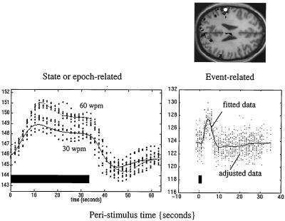
Since the advent of fMRI a new distinction has emerged in neuroimaging; namely, that between event- and state-related measurements. By virtue of the half-life of the radioactive tracers used in positron emission tomography (PET), we have been confined largely to studying differences in brain states engendered by the repeated presentation of stimuli or the enduring performance of some task. With fMRI new techniques currently are being developed that allow the evoked responses to single stimuli or events to be characterized and compared. This is of fundamental importance for experimental design, because the facility to present experimental trials in isolation frees one from the potentially confounding effects of things like attentional set. For example, we now can look directly at the brain’s responses to novel events in “odd ball paradigms” and, more generally, disambiguate the effects of a particular stimulus from the context in which that stimulus was presented (see below). Fig. 7 makes a distinction between state- and event-related brain responses by using a single-subject fMRI study in which the subject was asked to listen to words presented at a fixed rate over an extended period of time or to single words presented in isolation. These analyses represent a simple version of the Volterra series approach described above and rely on the use of temporal-basis functions. Event-related fMRI now presents the opportunity to adopt the same sorts of experimental designs that have proved so useful in evoked-potential work in electrophysiology.

Figure 7.

The data above were acquired from a single subject using echo planar imaging (EPI) fMRI at a rate of one volume image every 1.7 sec. The subject listened to words in epochs of 34 sec at a variety of different frequencies. The fitted periauditory responses (lines) and adjusted data (dots) are shown for two rates (30 and 60 words per minute) on the left. The solid bar denotes the presentation of words. By removing confounds and specifying the appropriate design matrix, one can show that fMRI is exquisitely sensitive to single events. The data shown on the right were acquired from the same subject while simply listening to single words presented every 34 sec. Event-related responses were modeled by using a small set of temporal basis γ functions of the peristimulus time. The SPM(F) shown, reflecting the significance of these event-related responses, has been thresholded at P = 0.001 (uncorrected) and displayed on a T₁-weighted structural MRI.

Context-Sensitive Responses in PET.

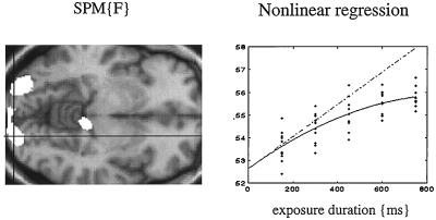
Perhaps it is worth considering event-related PET. It is not necessary to measure individual responses to stimuli to make inferences about them. We will briefly review two examples where PET has been used to examine the transient responses evoked by words, and where these responses have to be considered in light of the context in which they were presented. In the first example, words were presented visually, at a fixed rate, during PET scanning (13). The only variable was the exposure duration of the stimuli, which varied between 150 and 750 msec. Responses in the extrastriate cortex showed a monotonic increase with exposure duration. By using this parametric design in conjunction with a nonlinear regression analysis, we were able to show that the evoked responses deviated from a linear relationship with relatively attenuated responses at longer durations (see Fig. 8). These observations have two potential explanations. First, extrastriate responses to visually presented stimuli are preferentially enhanced by attentional mechanisms when the stimuli are very brief. This interpretation was supported by the observation that activity in the anterior cingulate was maximal at the shortest exposure durations. The second explanation is that there is intrinsic adaptation during sustained visual presentation, resulting in a progressive fall in the average response with increasing exposure duration. These alternative explanations provide a good example of where event-related fMRI could be used to adjudicate between them. By repeating the experiment with event-related fMRI one can remove the attentional influences and determine whether adaptation does indeed occur.

Figure 8.

(Left) SPM(F) testing for the significance of a second-order polynomial regression of activity on the duration of visually presented words as measured in five normal subjects by using PET. Bilateral extrastriate regions are shown as white regions surviving a threshold of P = 0.05 (uncorrected) on a structural T₁-weighted MRI. (Right) An example of this regression for the voxel under the cross-hairs on the left. It can be seen that the observed response function deviates from the linear relationship that would be expected if the amount of neural activity evoked was proportional to the duration over which it was elicited.

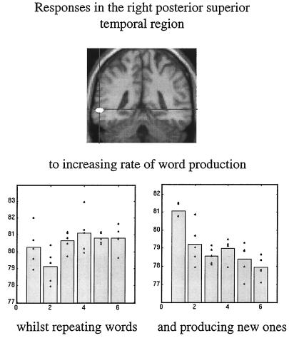
In the second example we asked subjects to produce words at a variety of rates. This was a factorial design, in that the words were either generated intrinsically, beginning with a heard letter, or extrinsically by simply repeating the letter. By looking for an interaction between the nature of word production and word production rate, we identified a region in the posterior temporal cortex that increased with extrinsically generated word rate and decreased with intrinsically generated word rate. The latter observation is remarkable and suggests that activity is reduced when more of these word production events occur. The only explanation for this is a true deactivation, or a reduction in brain activity, associated with the intrinsic production of each word (Fig. 9).

Figure 9.

Adjusted activity from a voxel in the posterior superior temporal region is shown as a function of word-production rate under the two conditions of extrinsic and intrinsic word generation. The change in the slope of these response functions under the two contexts is obvious. The voxel from which these data are derived is shown on the SPM(t) (Upper). These data come from a PET study of six normal subjects.

Context-Sensitive Activations and Interactions?

Many of the more compelling neuroimaging experiments have employed factorial designs, wherein the interaction among the factors used has been as interesting, if not more so, than the effects of the factors themselves. In terms of future trends, it might be anticipated that factorial designs will become more important. To the extent that brain responses are always more context-sensitive, then many effects that hitherto have been ascribed to simple activations by cognitive or sensory processes may in fact reflect interactions between these processes and the context in which they were elicited. Consider the following example. Imagine that we have discovered extrastriate activations when subjects viewed words as opposed to false-font letter strings. We might ascribe this activation to the difference between the stimuli and label the region as a “word-form area.” However, this regionally specific effect could be an interaction between implicit phonological retrieval and the visual processing of letter strings. To demonstrate this, one would need a factorial design in which the presence of letter strings was crossed with implicit phonological retrieval. On the basis of this experiment we might find that the region responded to the presence of letter strings relative to single characters and that this activation was enhanced by implicit phonological retrieval (when implicitly naming the word or letter). In other words, we could also construe this regionally specific effect as a modulation of letter string-specific responses by implicit phonological retrieval. In the absence of phonological retrieval, there may be no differences in the response of this area to words or nonword letter strings. This distinction between word-specific responses in an extrastriate region and word recognition-dependent modulation of extrastriate responses to any letter string is not a specious one. The two interpretations are that there are (i) “receptive fields” for words in extrastriate regions or (ii) a selective modulation of “receptive fields” for any letter string by higher cortical areas with “receptive fields” for the phonology of the stimulus. If we were able to inhibit the activity of these higher-order areas (using, for example, magnetostimulation), the extrastriate responses might no longer differentiate between word-like and non-word-like letter strings. If this were the case, should the extrastriate area be designated a word-form area? Clearly not in a simple way; however, it would constitute a necessary component of a distributed system involved in the perception of visually presented words. From a psychological perspective, one could posit a psychological component that was responsible for the integration of phonological retrieval and visual analysis. The interaction (e.g., that between phonological retrieval and the visual analysis of letter strings) would then represent an activation on comparing brain activity in states that did and did not have this integration. Factorial designs represent one way of identifying these integrative or context-sensitive activations. In summary, this example highlights the importance of regionally specific interactions and factorial designs. One interpretation of interactions is that they represent the integration of different processes (e.g., visual processing of letter stings and phonological retrieval) in a dynamic and context-sensitive fashion.

In conclusion, we have reviewed the importance of context-sensitive effects in neuroimaging both from the perspective of functional integration and effective connectivity and from the perspective of functional specialization and the integration of componential cognitive and sensorimotor processing. Advances in the design and analysis of brain imaging experiments are revealing the nature and role of these effects.

ABBREVIATIONS

fMRI

functional magnetic resonance imaging

PET

positron emission tomography

SPM

statistical parametric map

References

- 1.Friston K J, Price C J, Fletcher P, Moore C, Frackowiak R S J, Dolan R J. NeuroImage. 1996;4:97–104. doi: 10.1006/nimg.1996.0033. [DOI] [PubMed] [Google Scholar]
- 2.van Essen D C, Maunsell J H R. Trends Neurosci. 1983;6:370–375. [Google Scholar]
- 3.Kauffman S A. Origins of Order: Self Organization and Selection in Evolution. Oxford: Oxford Univ. Press; 1994. [Google Scholar]
- 4.Friston K J, Tononi G, Sporns O, Edelman G M. Hum Brain Mapp. 1995;3:302–314. [Google Scholar]
- 5.Lumer E D, Edelman G M, Tononi G. Cereb Cortex. 1997;7:228–236. doi: 10.1093/cercor/7.3.228. [DOI] [PubMed] [Google Scholar]
- 6.Friston K J, Frith C D, Turner R, Frackowiak R S J. NeuroImage. 1995;2:157–165. doi: 10.1006/nimg.1995.1018. [DOI] [PubMed] [Google Scholar]
- 7.Buechel C, Wise R S J, Mummery C, Friston K J. NeuroImage. 1996;4:60–66. doi: 10.1006/nimg.1996.0029. [DOI] [PubMed] [Google Scholar]
- 8.Friston, K. J., Josephs, O., Rees, G. & Turner, R. (1998) Magn. Reson. Med., in press. [DOI] [PubMed]
- 9.Friston K J, Ungerleider L G, Jezzard P, Turner R. Hum Brain Mapp. 1995;2:211–224. [Google Scholar]
- 10.Gerstein G L, Perkel D H. Science. 1969;164:828–830. doi: 10.1126/science.164.3881.828. [DOI] [PubMed] [Google Scholar]
- 11.Aertsen, A. & Preissl, H. (1991) in Non Linear Dynamics and Neuronal Networks, ed. (UCH, Schuster, H. G., New York), pp. 281–302.
- 12.McIntosh A R, Gonzalez-Lima F. Hum Brain Mapp. 1994;2:2–22. [Google Scholar]
- 13.Price C J, Friston K J. NeuroImage. 1997;5(4):S59. doi: 10.1006/nimg.1997.0269. (abstr.). [DOI] [PubMed] [Google Scholar]
- 14.Talairach J, Tournoux P. A Co-Planar Stereotaxic Atlas of a Human Brain. Stuttgart: Thieme; 1988. [Google Scholar]