Classification of Rotylenchulus reniformis Numbers in Cotton Using Remotely Sensed Hyperspectral Data on Self-Organizing Maps

Abstract

Rotylenchulus reniformis is one of the major nematode pests capable of reducing cotton yields by more than 60%, causing estimated losses that may exceed millions of dollars U.S. Therefore, early detection of nematode numbers is necessary to reduce these losses. This study investigates the feasibility of using remotely sensed hyperspectral data (reflectances) of cotton plants affected with different nematode population numbers with self-organizing maps (SOM) in correlating and classifying nematode population numbers extant in a plant's rhizosphere. The hyperspectral reflectances were classified into three classes based on R. renifomis population numbers present in plant's rhizosphere. Hyperspectral data (350-2500 nm) were also sub-divided into Visible, Red Edge + Near Infrared (NIR) and Mid-IR region to determine the sub-region most effective in spectrally classifying the nematode population numbers. Various combinations of different feature extraction and dimensionality reduction methods were applied in different regions to extract reduced sets of features. These features were then classified using a supervised-SOM classification method. Our results suggest that the overall classification accuracies, in general, for most methods in most regions (except visible region) varied from 60% to 80%, thereby, indicating a positive correlation between the nematode numbers present in plant's rhizosphere and the corresponding plant's hyperspectral signatures. Results showed that classification accuracies in the Mid-IR region were comparable to the accuracies obtained in other sub-regions. Finally, based on our findings, the use of remotely-sensed hyperspectral data with SOM could prove to be extremely time efficient in detecting nematode numbers present in the soil.

Rotylenchulus reniformis (Linford and Oliveira, 1940) is a plant-parasitic nematode widely found in sub-tropical and tropical regions around the world. It is a sub-tropical semiendoparasitic species in which vermiform females of R. reniformis penetrate into the roots of the host plant, altering the flow of nutrients and moisture uptake capacity of the host plants and severely affecting their growth (Blasingame et al., 2002; Lawrence et al., 2006, 2007). The above-ground effects on the host plant vary depending upon the type of host and the number of nematodes affecting it. One of the hosts severely affected by R. reniformis is cotton (Gossypium hirsutum). Rotylenchulus reniformis can reduce cotton yields by more than 60%, with annual losses running in millions of dollars (Kelley, 2003; Lawrence et al., 2004, 2006). In 2006, the estimated revenue loss in the US caused by R. reniformis nematode was greater than $252 million (Blasingame, 2007). Hence it is necessary to not only identify the presence of the nematode in the soil but also to determine its numbers. Early and proper identification of nematode numbers is necessary to initiate nematode management programs (Kelley, 2003; Lawrence et al., 2004). The current method for the identification of R. reniformis is to count nematode numbers after extraction from soil. This requires that cotton producers collect soil samples and send them to a laboratory for analysis. This is a time-consuming and an inefficient process. In this study, the authors make use of the above-ground effects on the cotton plant caused by different R. reniformis numbers to investigate correlations between nematode numbers and effects on cotton. These above-ground effects were recorded using remote sensing technology.

Remote sensing is a method of observing and acquiring information about the target's properties without physically coming in contact with the target (King, 2004). Many advanced remote sensing instruments (e.g., Analytical Spectral Devices (ASD) Fieldspec Pro handheld spectroradiometer) collect large amounts of spectral data distributed over a wide range of bands (wavelengths) of the electromagnetic (EM) spectrum. The hyperspectral data are collected over a range from 350-2500 nm and represent hundreds of discrete measurements of a target's reflected energy as a function of wavelength. (Lillesand et al., 2000; Kelley, 2003). Reflectance is a derived, dimensionless quantity and is defined as the ratio of the radiance reflected from the target under study to the radiance reflected by an ideal Lambertian surface in the same direction under the same illumination conditions. A plant's reflectance varies in different regions of the EM spectrum due to physical and chemical interactions of the energy with the plant. Reflectance in each region provides particular information about the plant. For instance, the radiance reflected by a plant in the visible region (350-700nm) is governed by plant pigments (e.g., chlorophylls or carotenoids), in the NIR region (700-1300 nm) the cellular structure of the plants governs the reflected radiance, and the Mid-IR region (1300-2500 nm) provides information about the moisture content present in the leaves of the plant (Lillesand et al., 2000). Information gathered from energy reflected across the spectrum can be used to assess the health of the plants and contributing stress factors. . Furthermore, there are certain specific bands that contain unique information about plants. Therefore, a wide range of hyperspectral observations might be useful in providing vital information in analyzing the effect of different nematode numbers on plants in different regions of the EM spectrum (Null, 2002; Kelley, 2003; King, 2004). It is also possible that different nematode numbers have varying effects on plants at different wavelengths. These effects may range from being extremely significant to subtle.

With the magnitude of a dataset of hyperspectral data, but not many training samples, the pattern recognition problem of associating a particular set of features (for our study, wavelengths of the hyperspectral data is considered as features) with a specific range of nematode numbers is challenging. In our study, the entire data set was divided into training and testing samples. Training and testing data samples are nothing but hyperspectral observations obtained from nematode infested cotton plants, where each wavelength of these hyperspectral observations forms the features. To seek a solution for the above discussed pattern recognition problem, an unsupervised Artificial Neural Network (ANN) architecture was considered.

An artificial neural network (ANN) is a simple layer of interconnected neurons. It iteratively adapts (trains) itself by changing its structure (neuron positions) according to the information provided to the network (Anderson and McNeil, 1992). This adaptation is accomplished by adjusting the strength of the network connections (weights) among neurons. The ANN can be trained either by supervised learning or by unsupervised learning. In supervised learning, the network is provided with both input (training data) and desired output. The network is trained in such a way that when the network is provided with the new data (test data), it gives an output very close to the desired output. If the desired output is not obtained, then the parameters used for training are varied accordingly until the desired output is achieved (Anderson and McNeil, 1992; Null, 2002; King et al., 2005). In unsupervised learning, only the input data is provided, and the network will solely classify the input data and present the classified data in a self-organized, meaningful way (Xin, 1999; Bin, 2004). The self-organized classification performed by ANN based on similarity in the input feature vector is called Self-Organized Maps (Anderson and McNeil, 1992; Xin, 1999; Duda et al., 2000; King et al., 2005).

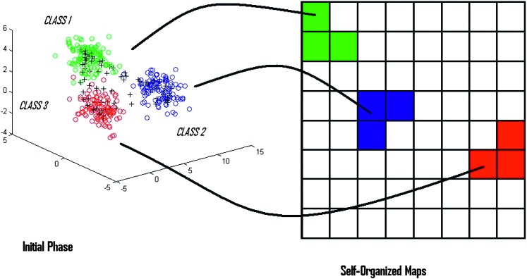
Principle and Working of Self-Organized Maps: Kohonen (1990) first introduced an unsupervised, self-ordering and competitive artificial neural map widely known as Self-Organized Feature Maps (SOFM), a.k.a., Self-Organized Maps (SOM). SOM is widely used in data clustering, pattern recognition and classification purposes. Self-organized maps are usually implemented on a 2-dimensional hexagonal or a rectangular grid (King et al., 2000). Map grid is the standard method used to visualize the SOM in output space. It is the projection of high-dimensional data onto a low-dimensional space. Map grids are either rectangular or hexagonal in shape (SOM Toolbox Documentation, 2003). SOM has a property of placing data exhibiting similar features in the same or a neighboring map unit, thereby performing pattern classification (Fig. 1) (Null, 2002; Bin, 2004; King et al., 2005). The main principle of SOM is its ability to not only compress the high-dimensional data into a low-dimensional grid (2-D grid), but also to maintain the relative distances among the data units present in the multi-dimensional data space (Null, 2002). Samples located far apart in high dimension will also be located far apart on the map (King et al., 2000). SOM basically involves two processes: Vector quantization and Vector projection (Vesanto et al., 1999; Bin, 2004). Each map neuron i is associated with d-dimensional codebook vectorsm_i = [m_i1 m_i2 m_i3.…m_id], where d is the dimension of an input vector. Each neuron is connected with the neighboring neuron by a neighborhood relation, which determines the structure of the map (Goncalves et al., 2005). During each training step, a sample vector x is randomly chosen, and the Euclidean distance between the input sample x and all the codebook vectors are calculated. The minimum distance between the input vector x and the codebook vector is a winning neuron for the given input sample and is widely called Best Matching Unit (BMU) (Vesanto et al., 1999; SOM Toolbox Documentation, 2003; Wu and Yen, 2003; Bin, 2004). Winning neuron can be computed using the following formula (Null, 2002):

(1)

where ‖.‖ is the distance measure. The input vector is then mapped on the location of the winning neuron (BMU), and the neighboring nodes are updated and moved closer towards or further away from the input vector (SOM Toolbox Documentation, 2003; Goncalves et al., 2005;). This adaptation is done according to the following formula (SOM Toolbox Documentation, 2003):

(2)

where h_bmui is a neighborhood function. A standard neighborhood function used is a Gaussian function (SOM Toolbox Documentation, 2003) given by:

(3)

where α(t) is a learning rate ranging between [0,1] that decreases with time, σ(t) is a Gaussian kernel, and ‖r_bmu-r_i‖² is the distance measure. The mapping of d-dimensional output vector (BMU) from input vector is called Vector quantization, while the process of representing output vectors (BMU) onto a low-dimensional (typically a 2-dimensions) hexagonal or rectangular grid is known as Vector projection (Vesanto et al., 1999; Wu and Yen, 2003; Bin, 2004). For this study, the entire analysis was performed using an expanded version of Null's (2002) SOMASDGUI (Doshi, 2007), created on MATLAB (The MathWorks Version 7.04) based on SOM toolbox 2.0 (available at www.cis.hut.fi).

Fig. 1.

Principle/Working of SOM. SOM identifies the similarities in input samples in high-dimension and places the input data exhibiting similar features onto the same or neighboring map units of low-dimensional map grid. Thus performing both the functions of pattern recognition and data compression.

The primary objective of this study was to investigate whether a correlation exists between the infected cotton plant's reflectance and the nematode numbers present in the plant's rhizosphere. This study examined the possibility of classifying hyperspectral data based solely on the nematode numbers estimated from the soil samples. In addition to the primary objective, the authors investigated the region in the EM spectrum where maximum classification accuracies can be obtained. To enhance the classification accuracies, the authors applied advanced feature extraction and dimensionality reduction methods (e.g., DWT, PCA and SOM-based method) to the hyperspectral reflectances. Furthermore, this work briefly explored the idea of combining standard feature extraction method with Self-Organized Maps to further reduce the extracted feature in order to improve classification accuracies.

Feature Extraction Methods: Hyperspectral data are usually high-dimensional. In our study, the dimension of hyperspectral data was 2050. (451-2500 nm) (2151 dimension). It is necessary to reduce the dimension of the data set when only few training samples are available in order to avoid the problem of “curse of dimensionality.” “The curse of dimensionality states that number of training samples of each class must be around ten times the number of features” (Nakariyakul and Casasent, 2004). It is also seen that reducing the dimension of the data tends to increase the classification accuracy significantly (Nakariyakul and Casasent, 2004). Therefore, the feature extraction methods are necessary in reducing the data dimensionality as well in maintaining important information from the signals (data). The various feature extraction and dimensionality reduction methods used for our study are discussed as follows:

• (i) Reflectance as Features: The hyperspectral signatures (reflectances) themselves are provided to SOM as features and are then also classified using SOM. No feature extraction and dimensionality reduction methods are applied to the hyperspectral ASD data.

• (ii) SOM-based Feature extraction (BMU-feature extraction): In 2002, Null made use of self-organized maps in extracting important bands from hyperspectral signatures in order to perform classification. In this method, once the map size is determined or user-defined, the Best-Matching Unit (BMU) is calculated for each d-dimensional input data sample. A Euclidean distance matrix between the input data vector and its best matching unit is calculated for all the input samples and is given by the formula as follows:

  (4)

  The size of the distance matrix is given by (the size of the map) X (dimension of input samples). For each map unit where the sample is placed, a range is calculated by the formula given as follows (Null, 2002):

  (5)

  The map unit with no samples placed has a zero value. An artificial threshold is generated for each range with a non-zero value. This artificial threshold depends on the percentage specified by the user where, the higher the percentage, the more the number of bands that are selected. Null (2002) used a range from 5 to 20%. For each percentage, classification accuracy was calculated. Features were selected that provided the best classification accuracies at a given percentage. The artificial threshold is given by the formula as follows (Null, 2002):

  (6)

  The main advantage of this method was that size of the map determines the number of features (bands). Therefore, based on the similarity in the data vector, SOM will place the samples onto the same or a neighboring map unit. The more the samples placed in the same map unit, the fewer the features will be selected for classification.

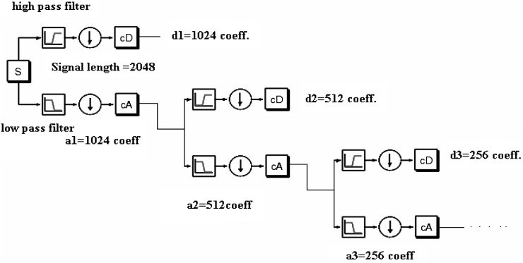
• (iii) Discrete Wavelet Transform (DWT): Discrete Wavelet Transform is a mathematical transform which dissects the signal into fine-scale and rough-scale information widely known as detail coefficients and approximate coefficients, respectively (Burrus et al., 1998; Bruce et al., 2002, 2003). Most wavelet systems that satisfy a multi-resolution approach (MRA) can project the signal into the shifted and scaled version of a basis function also known as mother wavelet (Burrus et al., 1998; Bruce et al., 2003). In this study since the hyperspectral signals are in wavelength, wavelength domain is considered instead of time domain (Bruce et al., 2003). The basis function for discrete wavelet transform (DWT) can be mathematically represented as:

  (7)

  Where ψ is the mother wavelet and λ is the wavelength. The factors a and b are used for dilation and shifting in the mother wavelet. The DWT is usually performed using an iterative dyadic tree (Fig. 2). According to the Mallat algorithm (Burrus et al., 1998), dyadic DWT could be implemented using successive series of high-pass and low-pass filters, whose filter design is determined by the type of the mother wavelet. To implement the dyadic DWT, it is assumed that the length of the hyperspectral signals (in terms of wavelength) is of power 2; if not, the signals are padded with zeroes to make the signals a power of 2. For instance, if the signal is of length N = 2048, one can have log₂ (N) or 11 decomposition levels. At each decomposition level, the signal is broken up into detailed coefficients (d) and approximate coefficients (a) with equal lengths. At the first decomposition level, length of approximation and detailed coefficient is N/2 = 1024. At the second decomposition level, a₁ is broken up into a₂ and d₂ having length N/4 = 512. Hence, at each decomposition level, the approximation coefficient is broken up into detailed and approximate coefficients. Bruce et al. (2002) used these coefficients as features for dimensionality reduction and classification purposes. According to them, simple mother wavelets perform better compared to higher order wavelets. Hence, for this study, detailed coefficients obtained using a Haar wavelet (Burrus et al., 1998), which is the simplest of all wavelets, were considered as features for classification purposes. Since large numbers of coefficient combinations could be used as features, this study limited its analysis to the following three combinations of detail coefficients for all the regions: Feature vector created from detail coefficients obtained from first three decomposition levels (F3C); Feature vector created from detail coefficients obtained from all decomposition levels (ADC); and Best Wavelet (detail) Coefficient (BWC) using automated process (coefficients from each decomposition level are given to the SOM, and the one with best accuracy was selected).

• (iv) DWT-BMU-based Feature Extraction: The use of detail coefficients (from all decomposition levels) as features contains most of the vital information about the signal, but the length of the feature vector is nearly same as the length of the hyperspectral signals, causing the problem of “curse of dimensionality” (Nakariyakul and Casasent, 2004). If the best wavelet coefficient(s) is (are) used, the sequence is considerably reduced, but it is possible to lose important information present in the other detail coefficients. In addition to that, if the best wavelet coefficient was from the first few decomposition levels, the coefficient sequence used is still large enough to cause the problem of “curse of dimensionality” (Nakariyakul and Casasent, 2004). If the manually selected detail coefficients from the first three decomposition levels are used as features for classification, the same problem of “curse of dimensionality” persists. In order to reduce the sequence dimensions as well as preserve important information from the sequence, the combination of DWT and SOM/BMU-based feature selection method is used (Moon and Merenyi, 1995; Campos and Carpenter, 1998; Logan, 1998; Cheong and Aggrawal, 2002; Doshi, 2007; Doshi et al., 2007a). In this approach, DWT was first applied to the ASD hyperspectral signals using a Haar mother wavelet. The signals were then decomposed into a series of detail and approximate coefficients to the maximum or user-defined decomposition level. At each decomposition level, only the detail coefficients were stored and concatenated with the previous detail coefficients to form a final output sequence consisting of series of detail coefficients. The approximate coefficients were discarded at all decomposition levels. The length of the sequence would be same as the length of the hyperspectral signal if the maximum decomposition level using a Haar wavelet is achieved. This sequence of detailed coefficients was then given to Null (2002) et al.'s SOM/BMU-based feature extraction and dimensionality reduction method to extract important coefficients, thereby reducing the dimension of the feature vector. The reduced feature vector was then used as feature classification purposes. In this study, SOM/BMU-based feature extraction method was applied to two variations of DWT: feature vector created from detail coefficients obtained from first three decomposition levels (F3CB); and feature vector created from detail coefficients obtained from all decomposition levels (ADCB).

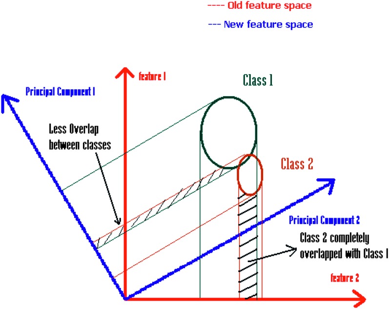
• (v) Principal Component Analysis (PCA): Principal component analysis is a standard statistical method widely used in agricultural and remote sensing applications to reduce the dimensionality of the data. It linearly transforms the data into a new feature space having its new axes orthogonal to one another (Duda et al., 2000; Bell and Baranoski, 2004). This transformation decorrelates the highly correlated remote sensing data, but maintains the maximum variability among them (Fig. 3). In PCA, a symmetric covariance matrix is computed, with each component indicating the correlation between the two variables of the data vector (Bell and Baranoski, 2004). From the covariance matrix, orthogonal bases are calculated using eigenvectors and eigenvalues based on matrix theory (Hollmen, 1996; Duda et al., 2000; SOM Toolbox Documentation, 2003). The eigenvectors are arranged in descending order of eigenvalues to transform the data into an orthogonal co-ordinate system, with the first few principal components having the highest amount of variability and retaining a significant amount of information from the data (Hollmen, 1996; Duda et al., 2000; SOM Toolbox Documentation, 2003). The remaining components could be discarded. In this way, PCA are widely used for feature extraction and dimensionality reduction.

  In the case of hyperspectral signal, the number of principal components is equal to the number of bands. For this study, the first four PCA components were considered and used as features for classification purposes.

• (vi) PCA-BMU-based Feature Extraction: In the standard PCA, as discussed above, only the first few components contain the majority of the variability. Therefore, only the first few components are selected, while the rest of the components are discarded. There are two disadvantages in using the above-discussed traditional procedure: selecting the best number of components as features for classification; and possibilities of eliminating higher-order components (with lower variance) that might be important/better for classification, especially in change detection applications. In order to prevent discarding important higher-order components and to avoid the problem of component selection, a combination of standard PCA with SOM/BMU-based feature extraction method was used for our data analysis. The procedure is to apply standard PCA to the reflectance of various classes. These PCA components are used as inputs for the Null's (2002) SOM/BMU-based feature extraction method. The output of this method would be the combination of both higher order as well as lower order PCA components that are useful in classification of different nematode classes. The extracted PCA components were then used as features in classification purposes (Rosado-Munoz et al., 2002; Mao, 2005; Doshi, 2007).

Fig. 2.

Dyadic DWT decomposition (originally acquired from Math works Inc, 2006 and modified in paint).

Fig. 3.

Principal Component Transform. The figure shows that shifting the axes maximizes class separability.

Materials and Methods

Data Collection: Cotton plants were grown in field microplots, located on the North Plant Sciences Research Farm at Mississippi State University. Microplots consisted of 76-cm diam. fiber-glass cylinders placed 45-cm deep in the soil. The soil was classified as a Freestone sandy loam (61.2%, 31.2%, 7.5%, Sand-Silt-Clay, pH 6.4). The entire test area was covered with a 6-ml thick plastic tarp and fumigated with methyl bromide [397 kg/ha (57:33; methyl bromide:chloropicrin)] 45 d prior to planting. The tarp was removed after 7 d, and the plots were allowed to air for 38 d prior to planting for each year. Each microplot was artificially infested with one of five initial (Pi) levels of a greenhouse-maintained culture of R. reniformis. Reniform nematode was collected from a field located in Thalahatchie Co., MS and propagated on cotton (PM 1218BR) in the greenhouse. After 60 d, plants were removed, and the nematodes were extracted from the soil by combined gravity screening and sucrose centrifugal floatation (specific gravity = 1.13) (Jenkins, 1964).

The initial population levels of Pi = 0, Pi = 500, Pi = 1,000, Pi = 1,500 and Pi = 2,000 R. reniformis juveniles and vermiform adult life stages per 100 cm³of soil were added to the appropriate microplot and incorporated into the soil. Cotton seeds were planted on raised linear rows at a rate of 5 seeds/0.31 meters linear row. The test was arranged in a randomized complete block design with five replications. Plants growing in each microplot were maintained through the season with standard production practices as recommended by the Mississippi Extension Service. Plants were monitored once every two weeks throughout the cotton growing season, and the parameters of plant height, soil temperature, canopy temperature and average relative humidity were recorded (Kelley, 2003). The ASD hyperspectral data were collected for each microplot using a Fieldspec Pro Spectroradiaometer with a 1.4 m fiber optic cable and 25° field of view (FOV). The ASD hyperspectral data consists of 2,151 bands ranging from 350-2500 nm. For the year 2001, the first hyperspectral readings were taken on 6 June 2001, 25 d after planting (DAP) (Doshi, 2007). The hyperspectral readings were taken from three cotton plants, one leaf/plant single cotton leaves, each located at three nodes basal from the apical portion of the plants in all microplots (Kelley, 2003). Hyperspectral reflectances were collected using a clamp-on tungsten filament (i.e., an artificial light source) used to minimize any variability caused by natural light and to eliminate unwanted atmospheric effects. The leaf target was totally enclosed and not subject to any other source of illumination. For each ASD reading, corresponding soil samples were collected 15.2 cm from the main stem of the same plant in each microplot. Samples consisted of six 2.5-cm-diam., 20-cm-deep soil cores. Samples in each microplot were bulked and a 100 cm³ sub-sample was extracted, and R. reniformis numbers were enumerated. The hyperspectral readings along with their respective soil samples were collected once every two weeks from all microplots. These dates included 19 June (33 DAP), 25 June (39 DAP), 10 July (54 DAP), 6 August (81 DAP) and 20 August (95 DAP) in 2001. Hence two files were generated, one file with the R. reniformis count, and another with the ASD hyperspectral data for the plants growing in a specific microplot at a given date. For the year 2006, the same methods and procedures used to infest the microplots in 2001 were repeated to conduct the tests. The same procedure was used to collect the corresponding hyperspectral readings. The hyperspectral readings along with their respective soil samples were collected on: 14 June (44 DAP), 21 June (51 DAP), 28 June (58 DAP), 5 July (65 DAP), 12 July (72 DAP), 26 July (86 DAP) and 2 August (93 DAP).

Data Analysis:

The hyperspectral (reflectance) data were divided randomly into three classes based solely on R. reniformis numbers. For the year 2001, there were 1,107 ASD hyperspectral data samples collected from the microplots, and for the year 2006 there were 551 samples. In our data set, the nematode numbers varied from 0 to around 6500 reniformis/100 cm³ soil. Different combination of classes (based on nematode numbers) were tried and their corresponding hyperspectral reflectances were given to unsupervised SOM. Before providing input to the SOM, wavelength bands 350-450 nm were removed due to the fact there is very little radiance from the sun in this region of the spectrum and it is highly affected by the atmosphere. The reflectance data collected in this part of the spectrum was very noisy, and so an a priori decision was made to exclude this data from the analysis. For our given data set, the three best distinguishable classes provided by unsupervised SOM were 0-1,500, 2,000-4,000 and 4,501 and above R. reniformis/100 cm³ soil (Table 1). There were two reasons in selecting the following classes: 1. An unsupervised map created from classes having these ranges gave the best separation compared to the other combination of classes. 2. All three classes had sufficient number of samples (hyperspectral signatures).

Table 1.

Division of classes based on Rotylenchulus reniformis numbers and labels assigned for each classes.

It should be noted that the nematode classes were separated by 500 nematodes/100 cm³ soil in order to avoid any overlapping that SOM may find between the classes. As explained earlier, the classes were initially divided randomly, as the authors wanted to observe whether separating the classes by 500 nematodes/100 cm³ soil increases the distinction between the three classes. In other words, the authors wanted to observe the correlation between the nematode numbers and its affect on hyperspectral reflectances (signals). By separating the classes by 500 nematodes/100 cm³ soil, we observed that the classes were more precisely distinguishable. Since there is no exact one-to-one correlation between nematode numbers and its effect on hyperspectral reflectance, it is difficult to precisely define classes. Hence by separating the classes by 500 nematodes, the authors are trying to delineate (or capture) the effect of increase in nematode numbers of the corresponding hyperspectral reflectances obtained from the leaves of the cotton plants. Hence, the two ranges that were removed from our analysis were 1001-1500 and 3501-4000 nematodes/100 cm³ soil. Therefore, the total number of ASD samples used in our data analysis were 1040 samples in year 2001 and 503 samples in year 2006.

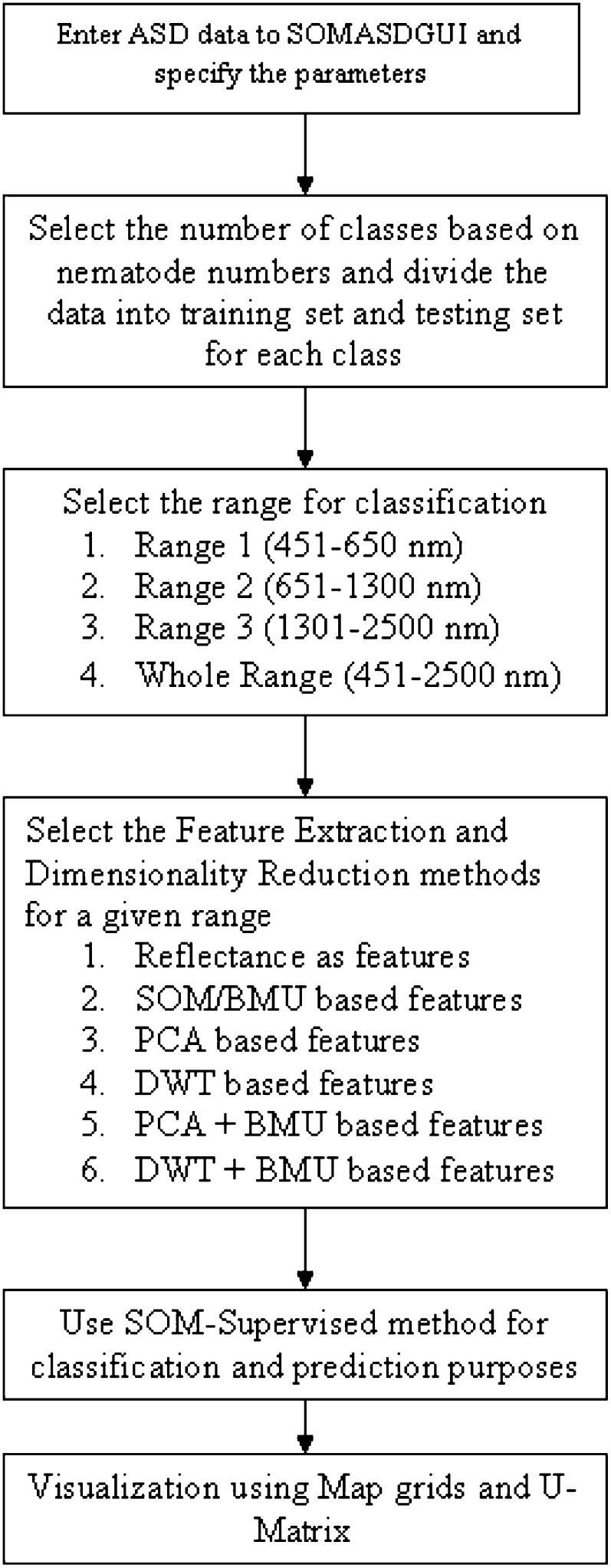
To investigate the EM region in which R. reniformis numbers most affected the cotton plants, the hyperspectral reflectances for all three classes were divided into three sub-regions (Table 2). Different above-mentioned feature extraction and dimensionality reduction techniques were applied to all the regions for all three classes. The features obtained from advanced feature extraction and dimensionality extraction methods were then provided to an expanded version of Null's (2002) SOMASDGUI, a MATLAB-based graphical user interface created in conjunction with SOM Toolbox (www.cis.hut.fi) for classification and visualization purposes (Fig. 4) (Null, 2002; Doshi, 2007). The idea is to initially select the number of classes based on the nematode numbers. Once the classes are selected, the hyperspectral signatures belonging to the particular classes are manually labeled. These labels assigned to the hyperspectral signatures are used for two purposes: (i) division of the data set between training and testing samples and (ii) representation of the output on the map. Once the data set is provided into the SOM, SOMASDGUI allows the user to enter the region and the type of feature extraction method to be applied on the given region. Classification accuracies are then computed based on supervised SOM classification method. The output is projected onto the map grid along with its U-matrix (Fig. 4) (Doshi, 2007). For our study, the classes were assigned different labels (Raaa-class 1, Raac-class 2 and Raca-class 3) (Table 1). The labels assigned for the different classes are solely for visualizing the location of the classes on the map-grid and have no meaning as such. For this study, the authors have manually color-coded each class (red-class 1, green-class 2 and blue-class 3) for better visualization.

Table 2.

Division of hyperspectral data into 3 sub-regions along with the entire region of study

Fig. 4.

Block diagram for working of the SOM Toolbox (figure partially acquired from SOM Toolbox Documentation and modified in MS-Paint).

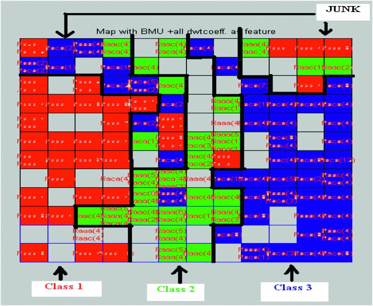
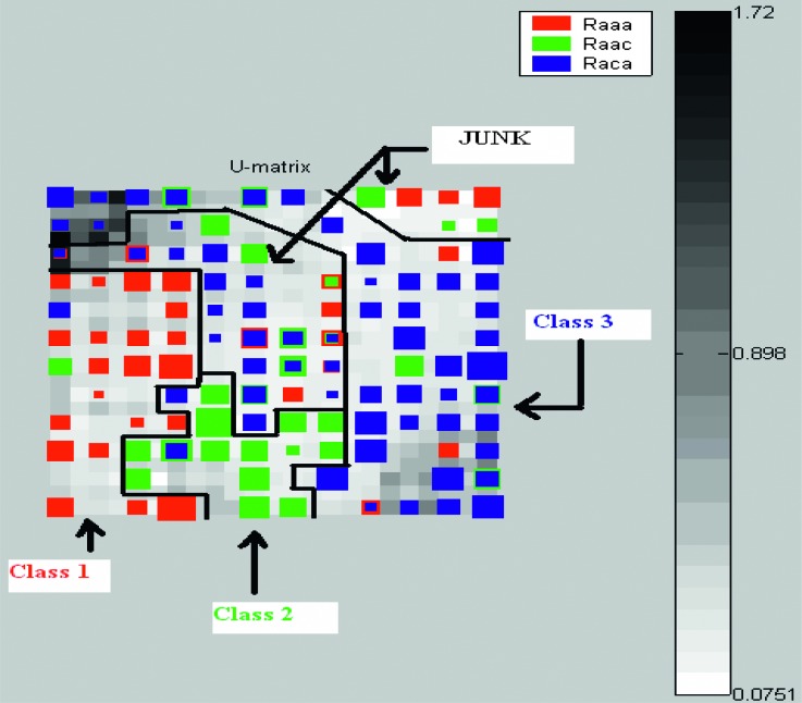
Visualization: Two types of visualization methods were considered: (i) Map grid: For this study, a rectangular-sheet type map grid was considered. The user specifies the grid size and shape, and then corresponding samples will be placed on the map depending upon their location in high-dimensional input space. Figure 5 shows the map grid created using features obtained from SOM/BMU method for the year 2001 in region 4. (ii) U-Matrix: Ultsch and Seimon (1990) first developed Unified Distance Matrix, also known as U-matrix, to visualize the distances between the neighboring neurons. It computes the distance between a given codebook vector and its adjacent neighbors and color-codes these distances onto the map (SOM toolbox Documentation, 2003). Darker colors in general indicate larger distances, thereby indicating the dissimilarities between neurons, while lighter colors indicate small distances. Darker areas in the U-matrix indicate cluster borders between the classes. The size of the U-matrix is (2X-1) x (2Y-1), where X and Y are the rows and columns of the map grid (Ultsch and Seimon, 1990). The U-matrix in Figure 6 is from an unsupervised learning of SOM using features obtained from SOM/BMU feature extraction method.

Fig. 5.

Map grid created using features obtained from SOM/BMU method for the year 2001. Classes are color coded as Red for class 1 green for class 2 and 3 blue for class 3. Color is assigned with the Map grid with maximum number of samples in the map unit. Junk part indicates the combination of all three samples or the samples whose signatures are distinctively different from the rest of the samples. Figure is modified in MS-Paint for better representation and visualization. Black borders are manually drawn to indicate distinction between classes.

Fig. 6.

U-matrix created using features obtained from SOM/BMU method. It is based on the map grid shown in Fig. 5. Figure is modified in MS-Paint for better representation and visualization. Black borders are manually drawn to indicate distinction between classes.

SOM Parameters: The features obtained from the various methods were classified and visualized after setting the SOM parameters. For this research work, the important SOM parameters were: Algorithm: Batch training algorithm; Initialization: Linear Initialization; Neighborhood function: Gaussian; Lattice: Sheet; Grid type: Rectangular grid; Training Data set: 75% of the total data set; Testing Data set: 25% of the total data set; Grid size: The grid size was determined by using the empirical formula given in SOM Toolbox. Some modification was made to the formula to obtain a square grid with nearly same number of map units as obtained from the empirical formulae of the SOM toolbox. The modified formula is given as follows (SOM Toolbox Documentation, 2003; Doshi, 2007):

(8)

Other Parameters: The other parameters such as learning rate, neighborhood function, length of training (learning), etc., were the same as default setting of SOM Toolbox.

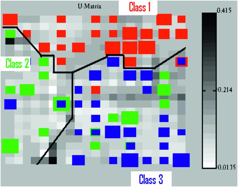
Classification: The hyperspectral reflectance of all three classes was divided into training and testing sets. Supervised SOM classification method was used in classifying the data. Supervised SOM algorithm is a slight modification of the original SOM in which an additional vector containing class information is added along with the dimension of the input vector (training data). The size of the additional class vector depends on the number of classes used for classification. For a given input sample, only one of the member components of the class vector has value ‘1’ while others have value ‘0’, thereby indicating the class of the input sample (SOM Toolbox Documentation, 2003). The class vector is not used to determine the Best Matching Units (BMU), only the input vector is used. However, to represent these BMU on to the map, only the information from the class vector is used (Hannula et al., 2003; SOM Toolbox Documentation, 2003; Xiao et al., 2005, Xiao et al., 2006; Doshi, 2007; Doshi et al., 2007b;). This causes a class-clustered map (Null, 2002). According to SOM Toolbox Documentation (2003), “the class of each map unit is determined by taking maximum over these added components, and a label is give[n] accordingly.” One of the advantages of using SOM for classification is that it will assign the map based on the number of the training samples in each class. The greater the number of the training samples in a particular class, the more the map units assigned to that class. Hence, once the class-clustered supervised map is created from the features obtained by applying various techniques to the hyperspectral reflectances and is projected onto the map, the same feature extraction techniques are applied to the testing data and are provided to the supervised map for class estimation. The testing samples are placed on the (trained) map based solely on the similarity of the features between testing and training samples. But since the classes of the testing samples are known in advance, the labels of testing samples are compared with the labels of trained SOM (supervised maps) and, based on their labeling, classification accuracies are calculated. In other words, accuracies are judged solely on the correct placement of testing sample placed on one of the three classes located on the map-grid. The total accuracies for each feature extraction method for each region were calculated as the weighted average of individual class accuracies. The U-matrix obtained using supervised-SOM algorithm using ADCB (DWT + SOM) feature extraction method in region 4 for the year 2006 is shown in Figure 7. From Figure 7, three distinct clusters are formed for the three classes with some overlap of class 2 with both the remaining classes. Darker areas in the figure indicate the cluster border for the given class.

Fig. 7.

U-matrix of the supervised SOM created using ADCB (DWT + SOM) as a feature extraction and dimensionality reduction method applied in region 4 for the year 2006. Figure is modified in MS-Paint for better understanding. Black borders are manually drawn to indicate distinction between classes.

Results and Discussion

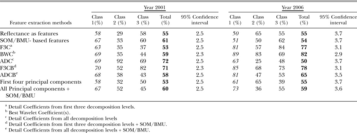
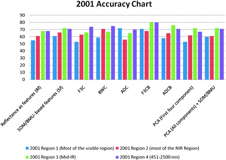
For the year 2001, for reflectances used directly as features and then provided to SOM-based architecture, classification accuracies were 55% and 61% in the visible and red edge + NIR regions, respectively, and 68% in the mid-IR region and for the Region 4 (all regions) (Tables 3-6), (Fig.8). Large feature set for small training data could be one of the reasons for lower accuracies when reflectances are directly used as features. Classification accuracies were slightly improved when Null's SOM-based method was applied to the hyperspectral reflectances (in various sub-regions). These were 61% and 66% in Visible and red edge + NIR regions, respectively, and 72% and 71% in Mid-IR region and Region 4, respectively (Tables 3-6), (Fig.8). This slight improvement in classification accuracies may have been due to the reduced set of features obtained from SOM-based feature extraction method, however, based the confidence intervals it was not possible to state whether the improvement was statistically significant or not. Application of Discrete Wavelet Transform gave mixed results. Classification Accuracies obtained using F3C combination of DWT as features were 53% and 63% in Visible and red edge + NIR regions and 66% and 74% in Mid-IR region and Region 4, respectively (Tables 3-6). Classification Accuracies using BWC combination of DWT as features were 59% and 71% in Visible and red edge + NIR regions and 67% and 75% in Mid-IR region and Region 4, respectively (Tables 3-6), (Fig.8). Classification Accuracies using ADC combination of DWT as features were 72% and 56% in Visible and red edge + NIR regions and 65% and 70% in Mid-IR region and Region 4, respectively (Tables 3-6). However, the use of various combinations (ADC, F3C and BWC) wavelet domain improves the accuracies in some regions but does not solve the problem of high-dimension. Hence, two combinations of DWT (ADC and F3C) were further subjected to Null's (2002) SOM-based method for dimensionality reduction. Classification accuracies for the features obtained from the combination of F3C and SOM-based method were 71% and 68% in Visible and red edge + NIR regions and 80% and 80% in Mid-IR region and Region 4, respectively (Tables 3-6), (Fig.8). Classification accuracies for the features obtained from the combination of ADC and SOM-based method were 58% and 65% in Visible and red edge + NIR regions and 76% and 71% in Mid-IR region and Region 4, respectively (Tables 3-6), (Fig.8). In many cases, the accuracies obtained using the combination of the detail coefficients from the first three decomposition levels (F3C) with SOM (i.e., F3CB) were higher compared to the accuracies obtained using combination of the detail coefficient from all decomposition levels (ADC) with SOM (i.e., ADCB) because according to Null's (2002) SOM-based feature extraction method, the maximum number of coefficients that can be selected depends on the size of map grid, therefore, only a limited number of coefficients are selected as best features for classification depending on the artificially generated threshold, and, for most of the cases, the best wavelet coefficient was from the first three detail coefficients.

Table 3.

Classification accuracies in visible region (451 nm – 650 nm) obtained for years 2001 and 2006 using various feature extraction methods.

Table 6.

Classification accuracies in entire region (451 nm -2500 nm) of study obtained for years 2001 and 2006 using various feature extraction methods.

Fig. 8.

Accuracy chart for the year 2001 for different feature extraction methods in different regions of EM spectrum.

The use of the first four lower-order PCA components as features via application of PCA in various regions of EM spectrum gave classification accuracies of 53% and 62% in visible and red edge + NIR regions and 72% and 71% in mid-IR region and region 4, respectively (Tables 3-6), (Fig.8). The use of PCA to reduce the dimensionality of data has two problems: selecting the number of components for analysis, and losing vital information present in higher-order PCA components. Combination of PCA with Null's (2002) SOM-based method solves both the problems. The use of PCA with SOM-based feature extraction method gave classification accuracies of 60% and 61% in visible and red edge + NIR regions and 72% and 71% in both mid-IR region and region 4 (Tables 3-6), (Fig.8).

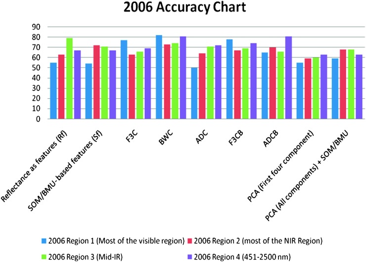
For the year 2006, the use of reflectances as features gave classification accuracies of 55% and 63% in Visible and red edge + NIR regions and 70% and 67% in mid-IR region and region 4, respectively (Tables 3-6), (Fig.9). When Null's (2002) SOM-based method was applied to reflectances, the classification accuracies were 54% and 72% in visible and red edge + NIR regions and 71% and 67% in Mid-IR region and Region 4, respectively (Tables 3-6), (Fig.9). The use of F3C as features produced classification accuracies of 77% in visible region, 63% in red edge + NIR region, 66% in mid-IR region, and 69% in region 4, respectively (Tables 3-6), (Fig.9). The use of BWC as features produced the classification accuracies of 82% in visible region, 73% in red edge + NIR region, 74% in mid-IR region and 81% in Region 4, respectively (Tables 3-6). The use of ADC as features produced the classification accuracies of 50% in visible region, 64% in red edge + NIR region and 71% and 72% in both mid-IR region and in region 4, respectively (Tables 3-6) (Fig.9). Classification accuracies for the features obtained from the combination of F3C and SOM-based method varied from 78% and 67% in visible and red edge + NIR regions to 69% and 74% in mid-IR region and region 4, respectively (Tables 3-6), (Fig.9). For the year 2006, combination of ADC with SOM-based feature extraction method produced classification accuracies of 65% in visible region, 70% in red edge + NIR region, 66% in mid-IR region and 81% in region 4, respectively (Tables 3-6), (Fig.9). The use of first four components as features produced the classification accuracies of 55% in visible region, 59% in red edge + NIR region, 60% in mid-IR region and 63% in region 4, respectively (Tables 3-6), (Fig.9). Finally, the combination of PCA with SOM-based method produced the classification accuracies of 59% in visible region, 68% in red edge + NIR region, 68% in mid-IR region and 63% in region 4, respectively (Tables 3-6), (Fig.9).

Fig. 9.

Accuracy chart for the year 2006 for different feature extraction methods in different regions of EM spectrum.

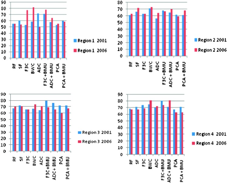
From the results (Tables 3-6), classification accuracies for the years 2001 and 2006 were nearly consistent (in terms of accuracy percentages) for all feature extraction methods in different regions of EM spectrum (except region 1) discussed in Table 2 (Fig. 10). This was also evident by observing the confidence intervals for the classification accuracies (Tables 3-6). The confidence intervals for each class's accuracies place each class's accuracies in the same range (West, 2006). Confidence intervals help one interpret whether accuracies in any particular region or group outperform any other particular region or group based on overlapping of the accuracy range between two groups or regions (West, 2006).

Fig. 10.

Accuracy comparison chart for the year 2001 and 2006 using different feature extraction methods in different regions of EM spectrum.

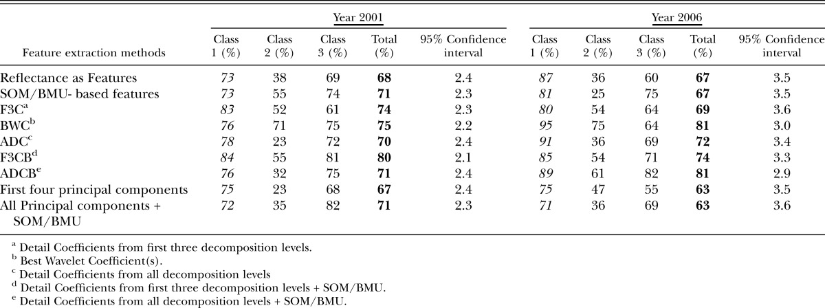
The overall classification accuracies for the three classes obtained using supervised SOM classification method in different regions of EM-spectrum for both years (2001 and 2006) using various feature extraction methods varied from upper 50% to lower 80% (Tables 3-6). This demonstrates that there is a positive correlation between the nematode numbers present in the plant's rhizosphere and the hyperspectral signatures (reflectances) collected from the corresponding plants. A plant's reflectance varies according to the nematode numbers present in the plant's rhizosphere. Classification accuracies of 60% to 70% could be considered fairly good given the fact that the classes were divided randomly, factors such as growth stage and days after planting were not taken into account, and the effect of nematodes on the reflectance was unknown. It is also evident that classification accuracies in the Mid-IR region were comparable to the accuracies obtained in the Visible and the red edge + NIR regions for most of the feature extraction methods for both years (Tables 3-6). This data indicates that R. reniformis numbers may not only affect the cellular structure of the leaves, but also the moisture-uptake capability of the plants (Lillesand et al., 2000; King, 2004; Doshi, 2007). Our study also shows that in most regions (except region 1), the classification accuracies obtained from the combination of SOM with standard feature extraction methods were nearly equal or exceeded the classification accuracies obtained from the traditional methods themselves. (Table 4-6). The only exception was for the year 2006 mid-IR region (region 3) where classification accuracy obtained using ADC (71%) outperformed the classification accuracy obtained using ADC + BMU (66%) (Table 5). It was also seen that even though the overall classification accuracies in spectral regions 2, 3, and 4 were about 60 and higher 70 percentile for most of the (except in region 2 for ADC feature extraction method for the year 2001 and PCA's first four components for year 2006) feature extraction methods, the individual classification accuracies for Class 1 in these three spectral regions (with nematode numbers less than or equal to 1,500 nematodes per cm³ soil) varied from 60% to lower 90% for both years in most cases. This result seems to be encouraging, given the fact that the threshold at which it is vital to start a nematicide management program for R. reniformis is in this range (Blasingame et al., 2002). Nematologists have established a population density of 200-250 nematodes/100 cm³ soil in spring and 1,000 nematodes/100 cm³ soil in fall as an economic threshold for R. reniformis (Blasingame et al., 2002). Once this density level is attained a management practice is warranted. This threshold is important because the cost of a nematicide management program above this threshold is less than the cost caused due to yield loss (Nova, 2001; Boyd et al., 2006). The results (Tables 3-6) also show that class 2 had the lowest accuracies in general, for both the years in different regions of the EM spectrum. This could be because class 2 had the least number of samples compared to the other two classes for both years.

Table 4.

Classification accuracies in red edge + NIR region (651nm-1300nm) obtained for the year 2001 and year 2006 using various feature extraction methods.

Table 5.

Classification accuracies in mid-IR region (1301 nm – 2500 nm) obtained for years 2001 and 2006 using various feature extraction methods.

Although class 3 accuracies varied from lower 30% to lower 80% for different regions using various feature extraction methods, most of the class 3 accuracies were in the range 55% or above for most of the feature extraction methods in all regions for both years. From Table 6, it is clear that the classification accuracies of class 3 was more than 60% in Region 4 for both years for all feature extraction methods except in year 2006,when PCA components were used as features for calculating classification accuracies (55%). We hypothesize that the accuracies for class 3 were lower compared to class 1 because, as the number of nematodes in the soil increases, there might be an ‘intra-specific competition’ between the nematodes (Koenning et al., 1996). We believe that since cotton roots are confined to restricted growth in the field microplot, it might reduce the effect of the nematodes on the cotton plant for a given period of time, thereby promoting the plant's growth, which in turn causes more class 3 samples to overlap with other two classes (Koenning et al., 1996). In other words, we believe that there is a positive correlation between the nematode numbers present in plant's rhizosphere with plant's hyperspectral reflectances. This means that due to ‘intra-specific competition’ between the nematodes, even though the number of nematodes in plant's rhizosphere is high, its effect on plant's reflectance might be low. This might cause SOM to misplace the class 3 samples into other two classes.

Finally, our research also suggests that the use of remote sensed hyperspectral data with the self-organized maps altogether provides a different and unique perspective in estimating different R. reniformis numbers. We theorized that this technique could prove extremely time-efficient in the sense that compared to the conventional means of calculating nematode numbers from soil, the above approach provides result in fairly shorter time (in hours). It should be noted that classes were exclusively grouped together in terms of nematode numbers present in the plant's rhizosphere at the time of data collection, while the growth and biomass of the plants at a given time were not taken into account. Hence it would be beneficial to classify the nematode numbers for a given date and time having uniform biomass. This might allow one to estimate the nematode number more accurately for a given biomass at a particular growth stage. Furthermore, it should be noted that although the results seem to be encouraging in classification of nematode numbers, it is necessary to validate the result with a larger set of data before putting it for practical and commercial use. However, the practical implementation of this approach is not without its challenges. The utilization of specific parts of the spectrum is the key to any practical instrument for field use. Any eventual measuring system is envisioned as a machine mounted unit that could be moved around a field at the appropriate growth stages for making strategic and economic nematicide applications. By mounting the measuring system on a tractor, the necessity of atmospheric corrections can be circumvented. As stated previously, reflectance is a derived quantity that has been normalized for a varying illumination conditions. The normalization process for ensuring reliable measurements for the tractor mounted system is envisioned to be similar to the methodology used with the handheld spectroradiometers used in this research. Finally, although much of this research focused on leaf measurements, the research team has also been conducting farm measurements of canopies. The results are encouraging and therefore, it is deemed highly probable that an instrument for measuring nematode populations is feasible.

Literature Cited

- Anderson D, McNeil G. Artificial Neural Networks Technology. Data & Analysis Center for Software. 1992 Online: http://www.dacs.dtic.mil/techs/neural/neural_ToC.html. [Google Scholar]
- Blasingame D, Gazaway W, Goodell P, Kemerait R, Kirkpatrick T, Konning S, Lawrence GW, McClure M, Mueller J, Newman M, Overstreet C, Phipps P, Rich J, Thomas S, Wheeler T, Wrather A. Cotton nematodes: Your hidden enemies. National Cotton Council; Memphis, TN. 2002. [Google Scholar]
- Blasingame D. Cotton disease loss estimate. Proceedings of the National Beltwide Cotton Conference. 2007 National Cotton Council, Memphis TN 1. Online: www.cotton.org/beltwide/proceedings. [Google Scholar]
- Bell IE, Baranoski GVG. Reducing the dimensionality of plant spectral databases. Proceedings of Institute of Electrical and Electronics Engineers on GeoScience and Remote Sensing. 2004;42:570–576. [Google Scholar]
- Bin Jiang. Extraction of Spatial Objects from Laser-Scanning data using a clustering technique. 2004 Online: http://www.isprs.org/istanbul2004/comm3/papers/270.pdf. [Google Scholar]
- Boyd ML, Phipps BJ, Wrather JA. University of Missouri-Columbia. Cotton Pests Scouting and Management. 2006 Online: http://muextension.missouri.edu/explore/agguides/pests/ipm1025insect.htm. [Google Scholar]
- Bruce LM, Koger CH, Jiang L. Dimensionality reduction of hyperspectral data using discrete wavelet transform feature extraction. Proceedings of Institute of Electrical and Electronics Engineers on GeoScience and Remote Sensing. 2002;40:2331–2338. [Google Scholar]
- Bruce LM, Cheriyadat A, Burns M. Wavelets: Getting perspective. Proceedings of Institute of Electrical and Electronics Engineers. 2003;22:24–27. [Google Scholar]
- Burrus CS, Gopinath RA, Guo H. Introduction to Wavelets and Wavelets Transforms. New Jersey: Prentice Hall; 1998. [Google Scholar]
- Campos MM, Carpenter GA. WSOM: Building adaptive wavelets with self-organizing maps. Institute of Electrical and Electronics Engineers World Congress on Computational Intelligence. Institute of Electrical and Electronics Engineers Proceedings on Neural Networks. 1998;1:763–767. [Google Scholar]
- Cheong WJ, Aggrawal RK. Accurate fault location in high voltage transmission systems comprising an improved thyristor controlled series capacitor model using wavelet transforms and neural network. Institute of Electrical and Electronics Engineers Proceedings on Transmission and Distribution Conference and Exhibition 2002 Asia Pacific. 2002;2:840–845. [Google Scholar]
- Costa JAF, De Andrade Netto ML. Cluster analysis using self-organizing maps. Proceedings of Institute of Electrical and Electronics Engineers SMC'99 Conference. 1998;5:367–372. [Google Scholar]
- Doshi RA. M.S. Thesis. Mississippi State University: Mississippi State; 2007. Self-Organizing Maps for classification and prediction of nemtatode populations in cotton. [Google Scholar]
- Doshi RA, King RL, Lawrence GW. Proceedings of Institute of Electrical and Electronics Engineers on Geoscience and Remote Sensing Symposium (IGARSS) Barcelona: Spain; 2007a. Wavelet-SOM in Feature extraction of hyperspectral data for classification of nematode species. July 2007. (in press) [Google Scholar]
- Doshi RA, King RL, Lawrence GW. Proceedings of Institute of Electrical and Electronics Engineers on Geoscience and Remote Sensing Symposium (IGARSS) Barcelona: Spain; 2007b. Self-organized maps-based spectral prediction of Rotylenchulus reniformis population numbers. July 2007. (in press) [Google Scholar]
- Duda RO, Hart PE, Stork DG. Pattern Classification. (2nd ed) Wiley: New York, NY; 2000. [Google Scholar]
- Goncalves ML, Netto ML, Costa J, Zullo J., Jr Automatic remotely sensed data clustering by tree-structured self-organizing maps. Proceedings of Institute of Electrical and Electronics Engineers on International Geoscience and Remote Sensing Symposium. 2005;1:502–505. [Google Scholar]
- Hannula M, Laitinen J, Alassarela D. Classification accuracy of the Frequency Analysis Method: Comparision between SOM-Supervised and k-NN. Proceedings of the 4th Annual Institute of Electrical and Electronics Engineers Conference on Information Technology Applications in Biomedicine. April 2003;254:257. [Google Scholar]
- Hollmen J. Process Modeling Using the Self-Organized maps data. M.S. Thesis. Helsinki University of Technology. 1996 Online: http://www.cis.hut.fi/jhollmen/dippa/dippa.html. [Google Scholar]
- Jenkins WR. A rapid centrifugal flotation technique for separating nematodes from soil. Plant Disease Reporter. 1964;48:692. [Google Scholar]
- Kelley AT. Mississippi State University: Mississippi State; 2003. Estimation of population thresholds of plant-parasitic nematodes on cotton using hyperspectral remotely sensed data. M.S. Thesis. [Google Scholar]
- King RL. Educational Resources: Intro to Remote Sensing Notes. 2004 Online: www.msstate.edu/∼rking/downloads. [Google Scholar]
- King RL, Rosenberger AL, Kanda LL. Artificial Neural Networks and Three-Dimensional Digital Morphology: A Pilot Study. International Journal of Primatology. 2005;76:303–324. doi: 10.1159/000089530. [DOI] [PubMed] [Google Scholar]
- King RL, Ruffin C, LaMastus L, FEShaw D. Classification of weed species using self-organizing maps. Proceedings of the 2nd International Conference on Geospatial Information in Agriculture and Forestry, Lake Buena Vista, FL. Erim International. 2000;2:151–158. [Google Scholar]
- Koenning SR, Walters SA, Barker KR. Impact of soil texture on the reproductive and damage potentials of Rotylenchulus reniformis and Meloidogyne incognita on cotton. Journal of Nematology. 1996;28:527–536. [PMC free article] [PubMed] [Google Scholar]
- Kohonen T. The Self-Organizing Map. Proceedings of Institute of Electrical and Electronics Engineers. 1990;78:1464–1479. [Google Scholar]
- Lawrence GW, Doshi RA, King RL, Lawrence KS, Caceres J. Nematode Management using Remote Sensing Technology, Self-Organized Maps and Variable Rate Nematicide Applications, World Cotton Research Conference-4. 2007 (in press) [Google Scholar]
- Lawrence GW, Kelley AT, King RL, Ellis GR, Vickery J, Lee HK, McLean KS. Remote sensing and precision nematicide application of Rotylenchulus reniformis management in Mississippi cotton. Nematode Monographs and Perspectives. 2004;2:13–21. [Google Scholar]
- Lawrence GW, King RL, Ellis GR, Doshi R, Lawrence KS, Caceres J, Samson S. Population estimation of the reniform nematode using hyperspectral reflectance data and applications to variable rate nematicide applications, Proceedings of the National Beltwide Cotton Conference, National Cotton Council, Memphis TN 1. 2006 Online: www.cotton.org/beltwide/proceedings. [Google Scholar]
- Lillesand TM, Kiefer RW. Remote Sensing and Image Interpretation. New York: John Wiley & Sons; 2000. [Google Scholar]
- Linford MB, Oliveira JM. Rotylenchulus reniformis, Nov.gen. n. sp., a nematode parasite of roots. Proceedings of Helminthological Society Washington. 1940;7:35–42. [Google Scholar]
- Logan MJ. Montana Tech of The University of Montana; 1998. Application of discrete wavelet transforms and self-organizing feature maps to classifying hyperspectral reflectance data. M.S. Thesis. [Google Scholar]
- Mao KZ. Identifying critical variables of principal components for unsupervised feature selection. Institute of Electrical and Electronics Engineers Transactions on Systems, Man and Cybernetics. Part B. 2005;35(2):339–344. doi: 10.1109/tsmcb.2004.843269. [DOI] [PubMed] [Google Scholar]
- Matlab Software: Math works Version 7.0.4. Online: http://www.mathworks.com/products/matlab/ [Google Scholar]
- Moon TS, Merenyi E. Classification of hyperspectral images using wavelet transforms and neural networks. Proceedings of Society of Photo Optical Instrumentation-Engineers (SPIE) 1995;2569:725–735. [Google Scholar]
- Nakariyakul S, Casasent D. Hyperspectral Ratio Feature Selection: Agricultural Product Inspection Example. Proceedings of Society of Photo Optical Instrumentation-Engineers (SPIE) 5587. 2004;5587:133–143. Online: http://www.ece.cmu.edu/∼casasent/5587-1622.pdf. [Google Scholar]
- Nova-Science in the news. Australian Academy of Science. August 2001. Integrated pest management – the good, the bad and the genetically modified. Online: http://www.science.org.au/nova/041/041key.htm. [Google Scholar]
- Null TC., II . Mississippi State University: Mississippi State; 2002. Use of self organized maps for feature extraction of hyperspectral data. M.S. Thesis. [Google Scholar]
- Rosado-Munoz A, Camps-Valls G, Guerrero-Martinez J, Frances-Villora JV, Munoz-Mari J, Serrano-Lopez AJ. Enhancing feature extraction for VF detection using data mining techniques. Institute of Electrical and Electronics Engineers Transactions on Computers in Cardiology. 2002;40:209–212. [Google Scholar]
- SOM Toolbox 2.0. 2005. Online: www.cis.hut.fi. [Google Scholar]
- SOM Toolbox Documentation. 2003. Online: http://www.cis.hut.fi/projects/somtoolbox/documentation/. Online: http://www.cis.hut.fi/projects/somtoolbox/package/docs2/somtoolbox.html. [Google Scholar]
- Ultsch A, Siemon HP. Dordrecht, Netherlands: Kluwer; 1990. Kohonen's self organizing feature maps for exploratory data analysis. Proceedings on International Neural Network Conference; pp. 305–308. [Google Scholar]
- Vesanto J, Himberg J, Alhoniemi E, Parhankangas J. Self-organizing maps in matlab: The SOM Toolbox. Proceedings of Matlab DSP Conference, Espoo. Finland. 1999:35–40. [Google Scholar]
- West TR. Mississippi State University: Mississippi State; 2006. Hyperspectral dimensionality reduction via sequential parametric projection pursuits for automated invasive species target recognition. M.S. Thesis. [Google Scholar]
- Wu Z, Yen GG. A SOM projection technique with the growing structure for visualizing high-dimensional data. Proceedings of the International Joint Conference on Neural Networks. 2003;3:1763–1768. doi: 10.1142/S0129065703001662. [DOI] [PubMed] [Google Scholar]
- Xiao Y, Clauset A, Harris R, Bayram E, Santago P, II, Schmitt JD. Supervised self-organizing maps in drug discovery. 1. Robust behavior with overdetermined data sets. Journal of Chemical Information and Modelling. 2005;45:1749–1758. doi: 10.1021/ci0500839. (Article) DOI: 10.1021/ci0500839. Online: http://pubs.acs.org/cgi-bin/article.cgi/jcisd8/2005/45/i06/pdf/ci0500839.pdf. [DOI] [PubMed] [Google Scholar]
- Xiao Y, Clauset A, Harris R, Bayram E, Santago P, II, Schmitt JD. Supervised self-organizing maps in drug discovery. 2. Improvements in descriptor selection and model validation. Journal of Chemical Information and Modelling46. 2006:137–144. doi: 10.1021/ci0500841. Online: http://pubs.acs.org/cgi-bin/article.cgi/jcisd8/2006/46/i01/pdf/ci0500841.pdf. [DOI] [PubMed] [Google Scholar]
- Xin Yao. Evolving artificial neural networks. Proceedings of Institute of Electrical and Electronics Engineers. 1999;87:1423–1447. [Google Scholar]