Sound-evoked network calcium transients in mouse auditory cortex in vivo

Abstract

Non-technical summary

The coherent activity of a large number of neurons forming functional cell assemblies crucially contributes to neuronal information processing in the brain. It is believed that activity of such populations constitutes a key mechanism linking awareness, stimuli from the external world, memory and behaviour. In this study, we recorded population calcium signals in the auditory cortex of mice using an optical fibre. We found that the population activity was dominated by transients lasting ∼1 s. These calcium transients directly reflected the action potential firing of local clusters of neurons and occurred spontaneously as well as in response to sound stimulation. We characterized in detail the spontaneous and sound-evoked calcium signals and the relation between the two. Thus, we were able to identify population calcium transients as an important element of sensory signalling.

Abstract

Population calcium signals generated by the action potential activity of local clusters of neurons have been recorded in the auditory cortex of mice using an optical fibre-based approach. These network calcium transients (NCaTs) occurred spontaneously as well as in response to sound stimulation. Two-photon calcium imaging experiments suggest that neurons and neuropil contribute about equally to the NCaT. Sound-evoked calcium signals had two components: an early, fast increase in calcium concentration, which corresponds to the short-latency spiking responses observed in electrophysiological experiments, and a late, slow calcium transient which lasted for at least 1 s. The slow calcium transients evoked by sound were essentially identical to spontaneous NCaTs. Their sizes were dependent on the spontaneous activity level at sound onset, suggesting that spontaneous and sensory-evoked NCaTs excluded each other. When using pure tones as stimulus, the early evoked calcium transients were more narrowly tuned than the slow NCaTs. The slow NCaTs were correlated with global ‘up states’ recorded with epidural potentials, and sound presented during an epidural ‘down state’ triggered a calcium transient that was associated with an epidural ‘up state’. Essentially indistinguishable calcium transients were evoked by optogenetic activation of local clusters of layer 5 pyramidal neurons in the auditory cortex, indicating that these neurons play an important role in the generation of the calcium signal. Taken together, our results identify sound-evoked slow NCaTs as an integral component of neuronal signalling in the mouse auditory cortex, reflecting the prolonged neuronal activity of local clusters of neurons that can be activated even by brief stimuli.

Introduction

Recording the electrical responses of single neurons is important for a better understanding of how neuronal circuits integrate incoming signals. However, studies of neurons one at a time are insensitive to neuronal population modes, which may reflect the activity of functional cell assemblies and contribute crucially to neuronal information processing (Bullock, 1997; Engel et al. 2001). For example, population modes possibly constitute a key mechanism linking awareness to sensory stimuli, memory and behaviour (Engel & Singer, 2001; Pesaran et al. 2002). To elucidate mechanisms of information processing at the level of the whole brain, it is necessary to characterize the dynamic structure of spontaneous and evoked population modes, and the relationships between the two (Harris et al. 2011).

Recently, due to the development of multi-cell bolus loading, the recordings of calcium signals became a major tool for studying neuronal populations in vivo (Stosiek et al. 2003). This technique allows the simultaneous staining of up to several hundreds of neurons and the surrounding neuropil by extracellular pressure application of a small molecule calcium-sensitive indicator dye. The calcium transients are then detected optically, e.g. using a 2-photon microscope. Using the same staining approach, a different readout method can be used: an optical fibre that is implanted in the stained cortical region delivers the excitation light to the tissue and transmits the fluorescent signal back to the detector unit where an integrated population calcium signal from the illuminated area is generated. This method has been shown to be suitable for monitoring of the average spiking activity of a local network of neurons (Adelsberger et al. 2005). This is due to the fact that the neuronal calcium transients are generally interpreted as the reflection of neuronal action potential firing whereas the neuropil calcium signal represents predominantly the calcium signal in axonal presynaptic structures. (Kerr et al. 2005; Garaschuk et al. 2006a; Rochefort et al. 2009). We call the recorded signals ‘network calcium transients’ (NCaTs). Notably, an optical fibre-based readout has been also successfully combined with genetically encoded calcium indicators (Lütcke et al. 2010).

Here, this approach has been used to study calcium signalling in the mouse auditory cortex. Mice have a complex set of communication calls (Holy & Guo, 2005) and important auditory behaviours, including the well-studied responses of mothers to the calls of their pups (Ehret, 2005). Their auditory system is similar to that of other high-frequency mammals: they don't hear much below 1 kHz but their hearing range extends well into the ultrasonic range. Studies using extracellular recordings have established that the mouse auditory cortex includes a number of fields, with largely tonotopically organized core fields (the primary field (A1) and the anterior auditory field (AAF), and multiple secondary fields) (Stiebler et al. 1997).

In this study, we characterize for the first time sound-evoked NCaTs in the mouse auditory cortex. Besides an early calcium transient that is consistent with the short-latency spiking response evoked by auditory stimulation (Sally & Kelly, 1988; Linden et al. 2003; Sakata & Harris, 2009), we describe here sound-evoked long-latency slow calcium transients. Experiments using two-photon calcium imaging followed by optical fibre recordings suggest that calcium signals recorded from neurons and the neuropil contribute about equally to the slow component of the NCaTs. We find that: (i) the slow sensory-evoked calcium transients share properties with the spontaneous calcium transients recorded in the absence of auditory stimulation and these two activity types mutually exclude each other; (ii) they are more broadly tuned for pure tone frequencies than the early calcium transients; (iii) they are related to global ‘up states’ measured by electrocorticography; and (iv) morphologically identical transients can be initiated by optogenetic activation of layer 5 pyramidal neurons, implying an intracortical mechanism for the initiation of the slow NCaTs.

Methods

Ethical approval

All experiments were carried out according to institutional animal welfare guidelines and were approved by the government of Bavaria, Germany.

Mice

For this study, Balb/c and transgenic mice expressing channelrhodopsin-2 (ChR2) under the control of the Thy1 promoter (Arenkiel et al. 2007) of either sex, aged between postnatal day 25 (P25) and 63 (P63), have been used. These mouse strains do not have hearing impairments at the ages used here, and are therefore a suitable model for auditory experiments (Turner et al. 2005).

Surgical procedure

All experiments were performed under isoflurane anaesthesia. There were no gas flow-induced sounds. Mice were initially anaesthetized by inhalation of isoflurane (Abbott, Wiesbaden, Germany) at a concentration of 1.5% in pure O₂. After inducing anaesthesia in a closed box the mice were transferred to a stereotaxic apparatus, placed on a warming plate (37°C) and gently fixed with ear bars during the surgical procedure. The depth of anaesthesia was verified by the lack of tail pinch and eye lid reflexes and by keeping the respiration rate at 80–120 min⁻¹. During the experiment the applied isoflurane concentration ranged between 0.8 and 1.2%. The eyes were protected by application of Isopto-Max creme (Alcon Pharma, Freiburg, Germany). Ten minutes after injection of 50 μl 2% xylocaine solution (Astra Zeneca, Wedel, Germany) under the scalp, the skin and muscles were removed with fine scissors. After drying the skull with air, the area where the fibre was to be fixed was treated with 37% phosphoric acid (Total Etch, Heraeus Kulzer, Hanau, Germany) for 15 s. After washing off the Total Etch with water and drying the skull with air, a mixture of Dentisive I and II (1:1 vol/vol) (Heraeus Kulzer) was applied. After 30 s Adhesive (Heraeus Kulzer) was added and hardened for 20 s with a UV lamp (Megalux, Mega-Physik Dental, Rastatt, Germany). A craniotomy was made above the core auditory fields of the auditory cortex, 2.5 mm posterior to bregma and 4.5 mm lateral to the midline.

Staining procedure

The staining solution was prepared as previously described (Stosiek et al. 2003; Garaschuk et al. 2006a). Briefly, stock solutions with a final concentration of 10 mm acetoxymethyl (AM) ester of the calcium-sensitive dye Oregon Green BAPTA-1 (OGB-1, Molecular Probes, Eugene, OR, USA) were prepared in DMSO containing 20% Pluronic F-127 acid. Prior to use these stocks were diluted in extracellular buffer containing (in mm) 150 NaCl, 2.5 KCl, 10 Hepes, yielding a final dye concentration of 1 mm. Five microlitres of the dye-containing solution were taken into a patch pipette connected to a pressure injection device (WPI, Berlin, Germany). The pipette was positioned at an angle of 60 deg (relative to the sagittal midline) and lowered from the surface of the cortex to a depth of 500 μm. The position of the pipette tip was measured from the surface of the cortex with a micromanipulator connected to the stereotaxic device. Up to 1 μl of the staining solution was gradually released into the brain by pressure application of about 7 kPa over 1–2 min. This procedure yielded a roughly column-like stained area through all cortical layers with a diameter of 400–800 μm.

Optical fibre recordings and activation of ChR2

The excitation of the dye, activation of ChR2 and detection of the fluorescence was performed by an experimental set-up similar to the one previously described (Fig. 1A) (Adelsberger et al. 2005). An optical fibre was used for delivering the excitation light from a 20 mW solid state laser (Sapphire, 488 nm, Coherent, Dieburg, Germany) to the previously stained brain region and for transmitting the fluorescence to the detector, in our case an avalanche photodiode (APD, S5343, Hamamatsu Photonics, Herrsching, Germany). It was possible to switch between two laser light intensities by means of an acousto-optic modulator (AOM 3080-125, Crystal Technology, Palo Alto, CA, USA): high intensities (about 2 mW at the tip of the optical fibre) for activation of ChR2 and low intensities (typically 0.01–0.1 mW at the tip of the optical fibre) for excitation of the calcium-sensitive dye and recording of the calcium-dependent fluorescence. For optical fibre recordings multi-mode fibres (FT-200-URT, Thorlabs, Grünberg, Germany) with a diameter of 200 μm and a numerical aperture (NA) of 0.48 were used. After removing the shielding from its tip the fibre was glued into a metal tube (0.9 mm o.d., about 10 mm length) with cyanoacryl glue (UHU, Buhl-Baden, Germany). The fibre tip protruded by about 1 mm from the metal tube. Approximately 30 min after dye application the fibre tip was inserted with a micromanipulator into the stained region to the depth providing maximal fluorescence intensity, typically at about 0–100 μm below the cortical surface. The metal tube was fixed to the skull with Charisma dental cement (Heraeus Kulzer), which was hardened for 20 s with UV light. At the end of the surgical procedure the ear bars were removed. During the recording the fibre was held loosely about 30 cm above the head of the animal. The fluorescent signal was then sampled at a rate of 1 or 2 kHz using an NI-PCI 6221 data acquisition card (National Instruments, Austin, TX, USA) and stored in files for offline analysis. Figure 1B shows a brain slice in which cells were loaded with a calcium-sensitive dye using the multi-cell bolus-loading technique. The image was taken with a CCD camera mounted on an upright microscope. The fluorescence is generated by laser light delivered by an optical fibre placed in parallel to the brain slice. The fluorescent region corresponds to the area from which population calcium signals were recorded.

Figure 1. Sound-evoked network calcium transients in the core fields of auditory cortex.

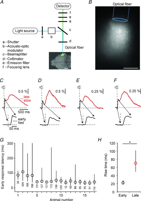
A, schematic of the experimental set-up for the optical fibre-based calcium recordings. The same fibre is used for delivering the excitation light (blue line) and guiding the excited fluorescence to the detector (green line). The overlay image of the excised brain indicates the area stained with calcium indicator dye. Scale bar, 2 mm. B, fluorescence excited by laser light delivered by an optical fibre placed parallel to a brain slice. Cells had been bulk-loaded with Oregon Green BAPTA-1 AM. The image was taken with a CCD camera mounted on top of a microscope and illustrates the area from which population calcium signals were recorded. Scale bar, 200 μm. C–F, average responses (average of 50 responses) to sound stimulation (100 ms broadband noise) in four different animals under isoflurane anaesthesia (shown as ΔF/F). Two components can be identified: an early fast-rising (black) and a late, slow-rising (red) calcium transient. The early part of the response is expanded below. G, the interquartile range of latencies for the early, fast-rising response to sound stimulation is shown for 17 recordings sites physiologically localized to the core fields of auditory cortex (A1 or AAF). Circles: median of the latency distribution. The range marked by the line includes half of all the latency values. The overall number of trials that were used in the analysis is marked below the data for each animal. H, rise time of the fast and the slow sound-evoked calcium transients (medians and interquartile ranges; n = 253 sound-evoked transients from 10 animals; Kolmogorov–Smirnov test, *P< 0.001). Please note that only transients starting from the fluorescence baseline level were included in this analysis.

Serial in vivo two-photon calcium imaging followed by optical fibre recordings

Animals were prepared for in vivo two-photon calcium imaging as described previously (Stosiek et al. 2003). The mice were placed onto a warming plate (37°C) and anaesthetized by inhalation of isoflurane. After injection of 2% xylocaine under the scalp, the skin and muscle were gently removed and a custom-made recording chamber was glued to the skull with cyanoacrylic glue. The mouse was transferred into the set-up and placed onto a warming plate. Continuous monitoring of the respiratory rate, heart rate and rectal temperature was performed. A small craniotomy (∼0.8 mm × 0.6 mm) was made above the auditory cortex using the same coordinates as reported for the optical fibre recordings. The recording chamber was perfused during the whole experiment with warm (37°C) extracellular perfusion saline containing (in mm): 125 NaCl, 4.5 KCl, 26 NaHCO₃, 1.25 NaH₂PO₄, 2 CaCl₂, 1 MgCl₂, 20 glucose, pH 7.4, when bubbled with 95% O₂ and 5% CO₂. The neurons were stained in vivo with the fluorescent calcium indicator dye Oregon Green BAPTA-1 (OGB-1) following the protocol described above. Forty-five to sixty minutes after dye injection two-photon calcium imaging was performed using a custom-built two-photon microscope based on a Ti:sapphire pulsed laser (DeepSee, Spectra-Physics, Newport, Irvine, CA, USA) and a resonant galvo-mirror (8 kHz; GSI) system (Sanderson & Parker, 2003). The scanner was mounted on an upright microscope (BX51WI, Olympus, Tokyo, Japan) equipped with a water-immersion objective (60×, 1.0 NA Nikon, Japan or 40×, 0.8 Nikon, Japan). Emitted photons were detected by photomultiplier tubes (H7422-40; Hamamatsu). Full-frame images at 480 × 400 pixel resolution were acquired at 30 Hz by custom-programmed software based on LabVIEW (version 8.2; National Instruments). At each imaging plane (n = 17 planes), we imaged spontaneous activity as well as sound-evoked activity. For simultaneous visualization of astrocytes labelled with sulforhodamine 101 and neurons labelled with OGB-1 the emitted fluorescence light was split at 570 nm. After the two-photon calcium imaging experiment we placed the optical fibre at the same recording site and recorded spontaneous as well as sound-evoked activity using the procedure described above (n = 7 animals).

Drug application

Bicuculline (100 μm; Sigma, Germany) was added to the extracellular saline solution perfusing a chamber attached to the mouse's skull (‘bath’ application) (Garaschuk et al. 2006b).

Electrocorticogram

For recordings of the epidural electrocorticogram, two silver wires (0.25 mm diameter; insulated except the nodular ends) were implanted epidurally 1 mm anterior to bregma/1 mm lateral to midline and 3 mm posterior to bregma/3 mm lateral to midline in the hemisphere ipsilateral to the optical fibre recording site and fixed with Charisma dental cement. A ground electrode was inserted into the neck muscles. Signals were detected with a differential amplifier EXT 10-2F (npi Electronic, Tamm, Germany), filtered at 0.1 Hz (high pass) and 1 kHz (low pass) and digitized at 2 kHz via a parallel channel of the acquisition card used for sampling the fluorescent signal. This configuration made it possible to record global ‘up states’ of the epidural potentials, although not the local electrical responses near the fibre. We used this arrangement to study the relationships between the calcium signals and the electrical activity (see Result section).

Sound stimulation

For stimulation pure tones or broadband noise were generated with LabView-based custom-written software and applied via a NI-PCI 6731 (National Instruments) sound card and an electrostatic speaker driver (ED1, Tucker Davis Technologies, Gainesville, FL, USA) with an ES1 free field speaker placed approximately 10 cm above the animal's head. Stimulus duration was 100 ms. Stimuli were presented with 10 ms rise and fall times. The interstimulus intervals were varied between 1 and 10 s according to the experimental requirements. Time marks at the start of each stimulus were stored in computer files together with the continuous fluorescence waveform and the epidural signals for offline analysis. The noise spectrum density in the room was measured using a 1/4 in microphone (Microtech, Gefell, Germany) connected to a B&K measuring amplifier type 2636. At high frequencies (>5 kHz) noise level was low; individual spectral lines did not exceed 20 dB sound pressure level (SPL). Pure tones were usually presented at the highest possible level without harmonic distortions. This level corresponded to about 70 dB SPL at most frequencies used here. In some experiments, sounds at lower levels were presented as well. The linearity of the sound stimulation was verified over a range of 40 dB. Broadband noise stimulation had a bandwidth of 0–50 kHz, and had the same overall energy as a tone at the same sound level. Thus, at the level usually used in the experiments, the noise had a spectrum level of about 23 dB/.

Post-recording documentation and data processing

At the end of the experiments, the animals were killed by inhalation of pure CO₂. The brains were removed and images were taken before and after slicing in order to document the exact position of the staining and recording region. Images were obtained using a PCO pixelfly CCD camera (pco.imaging, Kehlheim, Germany) mounted on an upright microscope (Zeiss Axioplan, Carl Zeiss, Oberkochen, Germany) or a dissection microscope. Fluorescent images were acquired using a fluorescein filter set and overlaid with the transmitted light images.

All data analysis of the optical fibre recordings was performed in Matlab (Mathworks) and IGOR Pro software (Wavemetrics, Lake Oswego, Oregon, USA). To correct for slow drifts of the baseline, the fluctuations of the fluorescence traces around their mean were first fitted by a 3rd degree polynomial (Fig. S1A in Supplemental material). The fit was subtracted from the trace, and the baseline was set at the 1st percentile of the subtracted waveform (so that 1% of the values were smaller from the baseline) (Fig. S1B). The fluorescence was transformed into ΔF/F units. Following these steps the fluorescence trace could still have appreciable amount of slow fluctuations at rates below 1 Hz, which presumably were not related to the sensory responses. To correct those, the data were decimated by a factor of 100 (to a rate of 10 or 20 Hz), and a lower envelope of the decimated signal was estimated by calculating, for each sample, the mean of the smallest five values in a symmetrical neighbourhood of 41 samples (corresponding to ±1 or ±2 s). The resulting trace was smoothed by a low-pass filter with a cut-off frequency of 2.5 Hz, up-sampled back by a factor of 100, and subtracted from the fluorescence trace (Fig. S1C). This adjusted fluorescence trace was used for all further analyses (Fig. S1D).

The calcium transients were located by a semi-automatic procedure that had a single adjustable parameter (described below). The adjusted fluorescence trace was low-pass filtered (corner frequency, 10 Hz). Candidate transients were identified by finding a local minimum and the following local maximum. Each candidate was characterized by its baseline fluorescence, its size and its maximum rate of rise. The final set of transients was selected based on two criteria. First, only transients that were larger than 10% of the dynamic range of the trace were considered. Second, the rate of rise of the transients (measured between the 10% and 90% points along their rising phase) had to be rapid enough. The distribution of the rates of rise of the candidate transients was usually bimodal, with a clear separation between slow and fast rise times. Only candidates with fast rise times were further considered. Since the boundary between slow and fast candidates depended on the baseline fluorescence (transients starting at higher levels tended to be smaller and slower), we used a plot of the rise time of each transient as a function of its baseline value to separate between them. On that plot, we set by visual inspection a linearly decreasing boundary between the two populations, for each recording separately. This procedure resulted in good fit with manually identified transients. Further analysis was performed on the adjusted fluorescence trace without the low-pass filtering used to detect the transients.

For identifying the epidural ‘up states’, the electrocorticogram signal was band-pass filtered between 2 and 40 Hz with a zero-phase filter (using the Matlab function filtfilt), squared, and low-pass filtered at 4 Hz with a zero-phase filter. Upward crossings of the median value of the resulting waveform were considered as transitions from a ‘down’ to an ‘up state’.

Analysis of the two-photon calcium imaging data was performed off-line in two steps. First, ImageJ (http://rsb.info.nih.gov/ij/) was used for drawing regions of interest (ROIs). Astrocytes were excluded from the analysis based on their selective staining by sulforhodamine 101 (Nimmerjahn et al. 2004; Garaschuk et al. 2006a), brighter appearance after staining with Oregon Green BAPTA-1 (Kerr et al. 2005) and their specific morphology with clearly visible processes. The presence of glial processes was assessed by inspecting z-stacks (stack of imaging planes located 70 μm below and above the imaged plane, distance between two focal planes, 2 μm) obtained routinely at the end of each experiment. In the next step, custom-made routines of the Igor Pro software (Wavemetrics, Lake Oswego, Oregon, USA) were used for the detection of calcium transients in individual neurons. Calcium signals were expressed as relative fluorescence changes (ΔF/F) corresponding to the mean fluorescence from all pixels within specified ROIs. For each ROI, a transient was accepted as a signal when its amplitude was greater than 3 times the standard deviation of the noise in the baseline. After the automatic analysis, all traces were again carefully inspected.

Localization of optical fibre recording sites

The position of the fibre was determined by stereotaxic coordinates, but the primary auditory cortex of mice is small (about 1 mm in diameter). We therefore used physiological criteria for localizing the recording locations by using response properties that are typical for the core auditory cortical fields (A1 and AAF). As we recorded from a single location in each animal it was not possible to assign the recording site to A1 or AAF. The properties we used to identify the core fields were response latency, frequency tuning and robustness of the noise responses presented at rates <1 s⁻¹. Recording sites in the core fields were expected to be narrowly tuned in frequency and to show short-latency non-habituating responses to noise bursts. In contrast, non-core sites were expected to be broadly tuned in frequency, have long response latencies, and to show habituating responses to broadband noise stimulation even at slow repetition rates. Using these properties, we identified 17 recording locations in the core fields and 5 recording locations in non-core auditory cortex. Six recording locations could not be categorized by these criteria because not enough stimulus conditions have been used. When both criteria could be tested, they were always congruent. Thus, we conclude that the majority of our recordings were in the core fields of the auditory cortex. Only data recorded from core fields according to these criteria were used for this study.

Estimation of the detection threshold of optical fibre recordings

To determine the number of active neurons necessary to generate NCaTs in vivo we combined two-photon microscopy and optical fibre recordings (Fig. S2 in Supplemental material). First we determined the number of cortical cells activated by local glutamate applications which were previously stained with the calcium indicator OGB-1. For this purpose we inserted a pipette filled with extracellular perfusion saline containing 100 mm glutamate and Alexa 594 into the centre of the stained region, at approximately 100–150 μm below the cortical surface (Fig. S2A). We verified the pipette position by quickly scanning in the two-photon imaging mode through various cortical depths. Once established, the pipette position was kept constant for the entire experiment. Then, using two-photon microscopy, we recorded at defined depths the calcium transients evoked by iontophoretic glutamate applications (50–100 ms). Figure S2B shows traces from seven neurons and two neuropil regions from the optical section at a depth of 155 μm. Only neurons and the neuropil region (shown are neuron 3–5 and neuropil A, respectively) that were affected by the glutamate application were responsive. In this whole section 21 cells and the neuropil located within the dashed white circle were activated by the glutamate pulses. In three consecutive applications, the same cells and the neuropil area A were responsive, indicating the robustness of the approach. Similar results were obtained in five additional optical sections of in this experiment (step size varied from 10 to 40 μm, depending on the cell density), covering the entire stained region. We checked carefully that each activated cell was assigned to a single optical section and that all cells of the stained region were tested. Each glutamate pulse activated an approximately ellipsoid-shaped cortical region with horizontal and vertical diameters of about 100 μm × 170 μm, respectively (Fig. S2A). In the entire cortical volume a total number of 90 active cell bodies were found in this particular experiment. In the following experimental step, an optical fibre was placed onto the cortical surface above the stained region. As the cortical region activated by the glutamate was much smaller than the diameter of the optical fibre, we can draw the conclusion that the optical fibre was capable of collecting signals from all active cells. In response to three glutamate pulses NCaTs were detected by the optical fibre (Fig. S2C). In Fig. S2D the number of active cells per glutamate application is plotted against the NCaT amplitude (data from 6 animals). The inset shows examples of NCaTs detected with the optical fibre from three different experiments. The amplitudes were linearly dependent on the number of active cells. Taken together, the activity of at least 20 active neurons (together with the surrounding neuropil) is necessary and sufficient to generate signals whose amplitudes were comparable to the ones of physiologically observed NCaTs.

Results

Sound-evoked network calcium transients in the core fields of auditory cortex

Figure 1C–F displays four examples of the network calcium transients (NCaTs) recorded in response to broadband noise stimulation in mice under isoflurane anaesthesia. The illustrated transients represent averages that were generated from at least 50 consecutive sound-evoked calcium transients. The sound-evoked NCaTs consisted of two components. The first component had a short latency and a fast rising phase. The onset latency of this component is quantified in Fig. 1G. It shows the distribution of onset latencies of the early calcium transient recorded from the core fields of the auditory cortices of 17 mice. The distribution of latencies for each animal is represented by its median (circle) and interquartile range (line connecting the 25% and 75% percentiles of the latency distribution). The short latencies of the early calcium transient are consistent with the onset latencies of calcium transients in single neurons as determined by electrophysiological recordings (Hromadka et al. 2008; Sakata & Harris, 2009). Following the fast component, the sound-evoked NCaT had a second component (Fig. 1C–F, red traces). This component had longer onset latencies and a slower rise time (defined as the time required for the signal to rise from 10% to 90% of its full amplitude) than the initial early response (Fig. 1H; n = 253 calcium transients from 10 animals, Kolmogorov–Smirnov test, *P< 0.001).

Spontaneous network calcium transients in the core fields of auditory cortex

NCaTs were also detected in the absence of auditory stimulation (Fig. 2A). These spontaneous NCaTs occurred with a mean frequency of 0.37 ± 0.04 Hz (n = 10 animals) and they resembled the sound-evoked slow long-latency calcium transients, which we recorded after noise stimulation. Figure 2B displays the average of 10 spontaneous (blue) and 10 evoked transients (black, early component; red, slow component) recorded in the same location. In this case, the rise times, widths and decay times of the spontaneous and the slow evoked calcium transient are rather similar. This was a general finding: the rise times, full widths at half-maximum (FWHM), and the decay time constants of both spontaneous and evoked slow transients were strikingly similar (Fig. 2C; n = 253 sound-evoked and 213 spontaneous calcium transients from 10 animals; Mann–Whitney test, rise time P = 0.07, FWHM P = 0.11, decay time constant P = 0.57).

Figure 2. Spontaneous network calcium transients resemble the late, slow-rising sensory-evoked calcium transients.

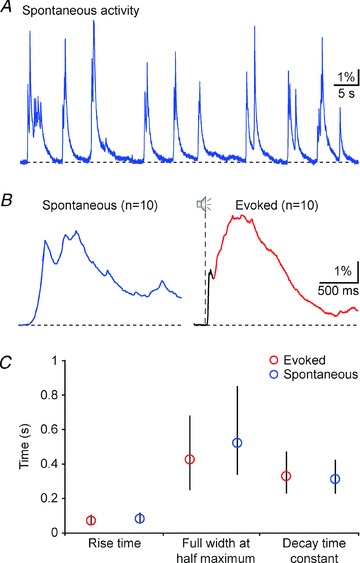
A, recording of spontaneous activity from the auditory cortex. B, average of 10 spontaneous (left panel) and 10 broadband noise-evoked (right panel) calcium transients, recorded from the same location. Note the difference in the temporal structure of the two averages. C, rise times, full widths at half-maximum, and decay time constants of the sound-evoked slow (red) and the spontaneous calcium transients (blue) (medians and interquartile ranges; n = 253 sound-evoked calcium transients from 10 animals; n = 213 spontaneous calcium transients from 10 animals; Mann–Whitney test, rise time P = 0.07, FWHM P = 0.11, decay time constant P = 0.57). Please note that only transients starting from the fluorescence baseline level were included in this analysis.

Comparison of optical fibre recordings and two-photon calcium imaging

In order to assess the cellular contribution to the sensory-evoked network calcium transients we performed two-photon calcium imaging of the auditory cortex neurons followed by optical fibre recordings from the same area (Fig. 3). Figure 3A and B compares two-photon microscopy and the optical fibre recording system. Two-photon microscopy provides optical sectioning capability and single cell resolution, but it is limited to the superficial cortical layers (Fig. 3A). The optical fibre system, however, records an average fluorescence signal from superficial as well as from deep cortical layers without providing single-cell resolution (Fig. 3B). For the combined two-photon and optical fibre experiments we used the same staining protocol used for the regular optical fibre recordings. Using two-photon calcium imaging we found – in line with previous studies (Stosiek et al. 2003; Kerr et al. 2005; Rochefort et al. 2009) – that this approach labels cells (neurons as well as astrocytes) and the surrounding neuropil. In analogy to the optical fibre system, which generates an average calcium signal (Adelsberger et al. 2005), we then analysed the average calcium signal recorded from one entire field of view containing both cells and the neuropil (full frame image of 120 μm × 120 μm). These full frame calcium signals were reliably present in response to sound stimulation (broadband noise, 100 ms long, every 5 s) as shown by an example of three consecutive trials (Fig. 3C, top) and the average of 10 trials (Fig. 3C, bottom). NCaTs recorded with the optical fibre from the same location had, as expected, two distinct components (Fig. 3D). Comparing these two signal types we found that the full frame calcium signals recorded with two-photon microscopy lacked the fast component of the sensory-evoked NCaTs while their time course was remarkably similar to that of the slow NCaTs (Fig. 3C and D, similar results from n = 7 experiments). This similarity between full frame calcium signals and slow NCaTs is most probably due to their similar origin as they are both a composite of cellular and neuropil calcium signal. This allowed us to use the full frame calcium signal as a surrogate to assess the relative contribution of the cells and the neuropil to the NCaTs. For this, we analysed the calcium signals recorded from three different regions of interest (Fig. 3E): (i) the full frame (blue continuous line), (ii) a region of interest containing all cells in the entire field of view (blue dashed circles) and (iii) the neuropil which consists of the remaining area. Figure 3F shows the calcium signals from these three regions of interest after sensory stimulation. We then calculated what proportion of the total fluorescence (represented as the fluorescence of the full frame image) the cells and the neuropil are contributing, respectively. In the example shown in Fig. 3F, 51% of the total fluorescence was generated by the cells whereas 49% of the total fluorescence was generated by the neuropil (Fig. 3G, left panel). In total, we analysed 17 imaging planes and found that the cells contribute on average about 43% of the total fluorescence (Fig. 3G, right panel). Because of the similar origin of full frame calcium signal and NCaTs we thus conclude that cells and the neuropil are also represented about equally in the NCaTs. Of course, this estimate is based on imaging planes located in cortical layer 2/3. Interestingly, we were not able to identify a correlate for the fast component of the NCaTs. This is probably due to the fact that the fast component is originating in the thalamo-recipient layer 4, which is not accessible for two-photon microscopy. The two-photon experiments suggest, however, that the slow component of the NCaTs may reflect the activity of a population of cells and the neuropil located in the remainder of the cortical column, for example also as shown in layer 2/3.

Figure 3. Comparison of optical fibre recordings and two-photon calcium imaging.

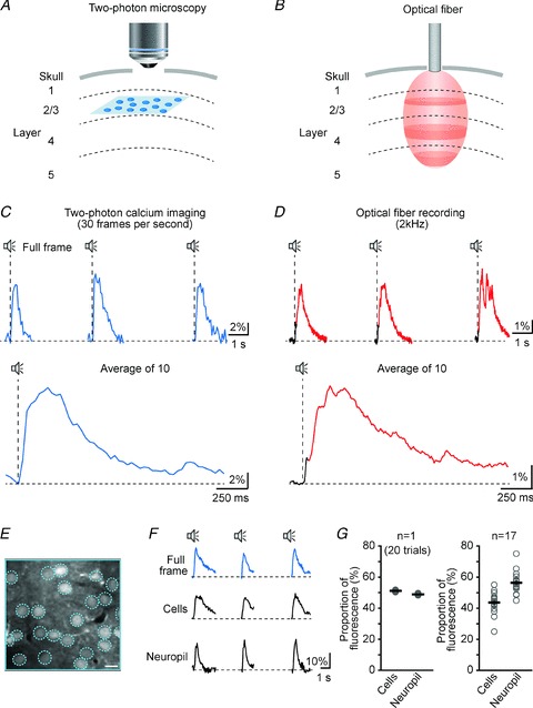
A and B, schematic representations of two-photon microscopy (A) and optical fibre recordings (B). Two-photon microscopy provides single-cell resolution, but is restricted to layer 2/3 (the blue area represents a typical imaging plane) whereas the optical fibre-based system is collecting an average fluorescence signal from superficial as well as from deeper layers (the red area represents the volume from which fluorescence is efficiently collected, see Fig. 1B). The dashed lines represent the cortical layer boundaries. C, sensory-evoked calcium transients recorded from one whole field of view (full frame image of 120 μm × 120 μm) using two-photon calcium imaging. Images were acquired at a frequency of 30 full frames per second. Upper panel: 3 consecutive trials. Lower panel: average of 10 consecutive trials. D, sensory-evoked network calcium transients (black: early fast-rising calcium transient, red: late slowly rising calcium transient) recorded with the optical fibre from the same staining site used for the two-photon imaging experiment shown in C. The sampling frequency was 2 kHz. Upper panel: 3 consecutive trials. Lower panel: average of 10 consecutive trials. E, in vivo two-photon image of cortical layer 2/3 of auditory cortex stained with the fluorescent calcium indicator dye Oregon Green BAPTA-1 AM. Scale bar, 10 μm. F, sensory-evoked calcium transients recorded from three different regions of interest. Top: whole field of view/full frame (blue frame in panel E). Middle: all cells present in the field of view (blue circles in panel E). Bottom: neuropil (remaining area). G, graphs showing the proportion of the total fluorescence (= fluorescence recorded from the full frame) generated by the cells and by the neuropil, respectively. Left panel: data from the imaging plane shown in E and F. Right panel: summary of 17 different imaging planes (20 trials each) from 8 experiments.

To address the question whether astrocytic calcium signals contribute to NCaTs we identified astrocytes based on their characteristic morphology or added in some experiments sulforhodamine 101, which selectively labels astrocytes (Nimmerjahn et al. 2004) (Fig. S3A in Supplemental material). We found that under our experimental conditions astrocytes were not spontaneously active at all (n = 11/19 astrocytes) or showed rare slow fluctuations (n = 8/19 astrocytes), which lasted for tens of seconds. This is in strong contrast to the neurons or even more the full frame calcium signal (Fig. S3B). The mean spontaneous frequency of astrocytic calcium transients was around 0.33 ± 0.09 transients min⁻¹ whereas calcium signals with a frequency of 27.1 ± 3.3 transients min⁻¹ were recorded from the full frame image (Fig. S3C, n = 8 experiments, Kolmogorov–Smirnov test, *P< 0.001). Similarly, during periods of auditory stimulation astrocytic calcium transients were rarely observed (mean frequency 0.10 ± 0.04 transients min⁻¹). Moreover, no temporal correlation with constant latencies between stimulus and subsequent transient could be found (Fig. S3D and E). In conclusion, under our experimental conditions astrocytic calcium signals do not contribute to NCaTs.

Relation between sensory-evoked and spontaneous NCaTs

Many electrophysiological recordings have shown that the spontaneous ongoing activity may affect sensory-evoked responses in auditory cortex and other cortical areas (Worgotter et al. 1998; Kisley & Gerstein, 1999; Edeline, 2003; Petersen et al. 2003; Castro-Alamancos, 2004; Sachdev et al. 2004; Curto et al. 2009; Marguet & Harris, 2011). To analyse the relationship between the spontaneous and the sound-evoked NCaTs, we studied sensory-evoked calcium transients evoked by sound stimulation during spontaneous transients. Figure 4A displays examples in which sound stimulation occurred at the peak (left), at the middle (middle) and at the end of the decay phase (right) of the spontaneous transient. The fast initial response (black) depended rather weakly on the fluorescence level at stimulus onset (see below). On the other hand, the increase in fluorescence due to the slow and long-latency component of the sensory-evoked calcium transient (red) depended strongly on the fluorescence level at stimulus onset. Figure 4A illustrates this dependence: the stimulus-dependent rise in fluorescence was small when the stimulus occurred at the peak of the preceding spontaneous calcium transient (left), recovered to its typical size when the stimulus occurred at the end of the spontaneous transient (right), and was intermediate when stimulation occurred at the middle of the decay phase (middle plot in Fig. 4A). Thus, the size of the sensory-evoked slow NCaT was a strongly decreasing function of the fluorescence level at stimulus onset. In fact, the evoked transient seemed to rise up to the typical peak fluorescence level of the spontaneous transient, but not beyond it, accounting for its dependence on the fluorescence level at stimulus onset, hence on the level of the neuronal activity at stimulus onset.

Figure 4. The amplitude of the sensory-evoked slow network calcium transients depends on the level of pre-stimulus spontaneous activity.

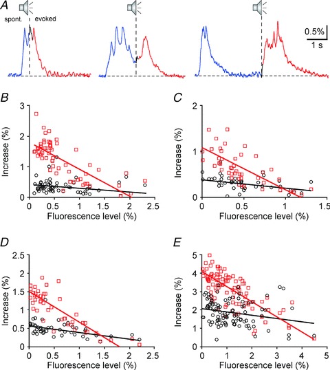
A, sound-evoked network calcium transients, elicited at different levels of fluorescence at stimulus onset. The stimulus was broadband noise of 100 ms duration. The amplitude of the late calcium transient depends strongly on fluorescence at stimulus onset. B–E, the amplitudes of the early (black circles) and the late (red squares) network calcium transients (quantified as increase in ΔF/F) are plotted as a function of fluorescence level at stimulus onset (quantified as ΔF/F). The regression lines are shown in the corresponding colours.

These observations are quantified in detail in Fig. 4B–E by plotting, for each trial, the maximal amplitude of the early transient (defined as the maximal increase in the response above pre-trial levels during the first 100 ms following stimulus onset, black circles) and the maximal amplitude of the late transient (defined as the maximal increase in the response above pre-trial levels starting 100 ms after stimulus onset, red squares) as a function of the average fluorescence level during the 100 ms preceding stimulus onset. While the early transients show only a slight decrease, if any, as a function of baseline, the late responses clearly decrease substantially more as a function of baseline. The regression lines through the maximal amplitude of the late transients (red lines in Fig. 4B–E) have a slope close to –1, showing that the maximum rise of the fluorescence above its level at stimulus onset reached approximately a fixed maximal level.

The generality of these observations was determined by analysing 63 recordings in 21 animals in which the responses to broadband noise have been measured. In all of these animals, at least one recording showed significant responses to noise, defined here as a significant difference (t test with P< 0.05) between the average fluorescence in the 500 ms intervals before and after stimulus onset; different conditions varied in the interstimulus interval and sound level, and in some conditions the responses were not significant. In all the cases that had significant responses (58/63, 92%), the amplitudes of the early and late transients were separately regressed against the fluorescence level at stimulus onset. Both early and late transients decreased as a function of fluorescence level at stimulus onset. However, the dependence of the early transients was rather weak. The average slope for the early transients was –0.09 ± 0.13%/% (mean ± SD; t =–5.3, df = 57, P < < 0.001; the units are % change in the size of the early transient for an increase of 1% in the fluorescence at stimulus onset). It was negative in 41/58 cases (71%) and significantly smaller than 0 in only 18/58 cases (31%). In comparison, the average slope for the dependence of the late transient on fluorescence at stimulus onset was much larger. Its average was –0.77 ± 0.16%/% (mean ± SD; t =–37, df = 57, P< < 0.001). It was negative in all cases (100%) and significantly smaller than 0 in 55/58 cases (95%). In addition, the average slope of the late transient was significantly larger than the average slope of the early transient (t =–25, df = 114, P< < 0.001).

Thus, while the early transient showed a weak (although significant at the population level) dependence on the fluorescence level at stimulus onset, the late transient was essentially always strongly dependent on the fluorescence level at stimulus onset, decreasing in size with increase in baseline calcium level.

To exclude the possibility that very small slow NCaTs evoked at the peak of the spontaneous NCaTs were due to the saturation of our detection system in four experiments we applied bicuculline, a GABA_A receptor antagonist, which has been shown to cause epileptiform neuronal activity including strongly increased action potential firing (e.g. Chervin et al. 1988; Schroeder et al. 1990; Badea et al. 2001). The aim was to generate NCaTs whose amplitudes exceeded those of the physiologically observed ones. Indeed, bath application of bicuculline revealed NCaTs which had on average a 4.7 times larger amplitude (3 ± 0.5%ΔF/F vs. 12.4 ± 2.6%ΔF/F; n = 4 animals, 50 transients per condition, Kolmogorov–Smirnov test, *P< 0.05) than the NCaTs observed under physiological conditions (Fig. S4 in Supplemental material).

Pure-tone-evoked network calcium transients

Broadband noise stimulation elicited significant responses in all recording locations. In order to address the question whether NCaTs also showed specificity to the sound frequency we applied pure tone stimulation. We found that the fast component of the NCaTs had remarkable frequency specificity in many cases. In the first row of Fig. 5A–C, 10 individual transients (grey lines) and their average (red line) which were recorded in three different mice in response to pure tone stimulation are displayed. These three examples were selected to demonstrate the range of observed best frequencies. The second row of Fig. 5A–C shows similar transients evoked in response to a frequency away from the best frequency. All example traces have been selected to be close to baseline fluorescence at stimulus onset. In the third row of Fig. 5A–C, the average traces in response to the two frequencies are compared directly over an expanded time scale. In all three examples, a distinct fast component was apparent at best frequency while the responses to a frequency away from the best frequency had longer latency and lacked the fast component. Thus, in these examples, while the fast component was present only in a relatively narrow frequency range around best frequency, slow NCaTs were evoked in response to many more frequencies. The average responses to all tone frequencies that have been tested in the three mice are displayed as ‘response planes’ in the fourth row (Fernald & Gerstein, 1972). Response planes display the response size (in colour) as a function of time (along the abscissa) and tone frequency (along the ordinate). All cases show tuned responses – rapid, maximal responses were evoked by frequencies within a restricted frequency band only.

Figure 5. Pure tone-evoked network calcium transients.

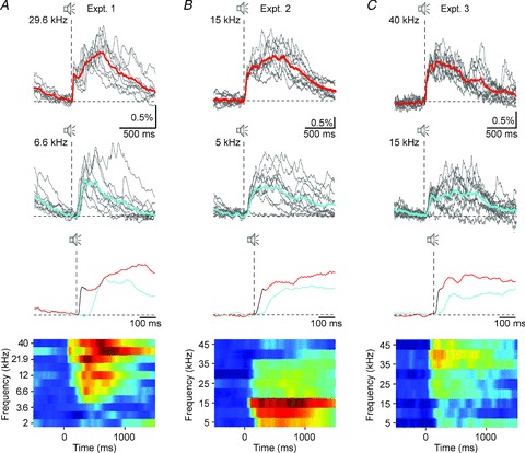
A–C, responses to pure tone stimulation found in 3 different recording sites. The examples were selected to illustrate the range of best frequencies that were observed. First row: 10 single responses and their average (cyan) to pure tone stimulation at best frequencies: A, 29.6 kHz; B, 15 kHz; and C, 40 kHz. Second row: 10 single responses and their average (cyan) to pure tone stimulation at off-best frequencies: A, 6.6 kHz, B, 5 kHz; and C, 15 kHz. Third row: enlarged view of the averages. The fast component is drawn in black. Please note the difference in latency, rise time and morphology between the responses to the best frequency and the off-best frequency. Fourth row: response planes displaying the response size (in colour) as a function of time (along the abscissa) and tone frequency (along the ordinate). The colours correspond to fluorescence levels between –0.1% (blue) to 1.1%ΔF/F (red).

We determined the range of frequencies that evoked any response (fast or slow NCaTs), and the range of frequencies that evoked a fast component in 42 response planes from 11 animals. Response planes within animals varied in the sound level at which they were taken and in the rate of presentation of the tones. In the majority of the response planes (36/42, 86%, present in all 11 animals) at least one frequency evoked fast, short-latency transients. The frequency range that evoked short-latency transients averaged 0.9 octaves, but had a highly skewed distribution: the median was 0.67 octaves, and 27/36 cases had a frequency range smaller than 1 octave. Tuning width of units in the auditory cortex of the mouse is similarly distributed (Linden et al. 2003).

The range of frequencies that evoked slow NCaTs was the same or larger than the range of frequencies that evoked fast transients (since fast transients were invariably followed by slow NCaTs). In the majority of the cases (30/42, 71%, at least one case in each one of the 11 animals), this frequency range was narrower than the full range of frequencies tested. Thus, the slow NCaTs also showed clear tuning in spite of their substantially larger bandwidth (average bandwidth, 2.3 octaves).

Network calcium transients in the auditory cortex and epidural potentials

While the early calcium transient most probably corresponds to the short-latency spiking responses typical of the auditory cortex, the electrical counterpart of the late component of the NCaT is unknown. We hypothesized that it represents a global ‘up state’ of higher activation spreading over large brain areas. In order to test this hypothesis, we recorded a brain-wide epidural electrocorticogram (ECoG) in five mice. Figure 6A shows a typical simultaneous recording of spontaneous activity of the epidural potential (lower panel) and the calcium signal (upper panel). The epidural potential showed the expected transitions between periods of activity and periods of network silence, the so-called slow waves which have a frequency of <1 Hz (Crunelli & Hughes, 2010). These have been shown to be associated with up–down state transitions in the membrane potential of single neurons (Steriade et al. 1993b; Doi et al. 2007). In our recordings, the slow waves corresponded to a substantial degree with the occurrence of the spontaneous calcium transients. Figure 6B shows an individual pair of a spontaneous NCaT (upper panel) and the simultaneously recorded epidural potential (lower panel). While the duration of the two is about the same, the calcium transient was slightly delayed relative to the onset of the epidural ‘up state’. This timing relationship was typical for spontaneous activity. Figure 6C shows the normalized cross-correlation between the calcium signal and the epidural potentials during spontaneous ongoing activity, calculated for the recording shown in Fig. 6A. The cross-correlation function has a clear peak near zero, slightly shifted to positive delays (corresponding to calcium signals following epidural potentials), as expected from the example in Fig. 6B. Indeed, among 74 calcium transients identified during recordings of spontaneous activity, 81% (60/74) occurred during an ‘up state’. This tendency was highly significant (χ²= 28, df = 1, P = 9 × 10⁻⁸). Thus, during ongoing activity, calcium transients followed quite consistently the epidural ‘up state’.

Figure 6. ECoG slow waves and network calcium transients.

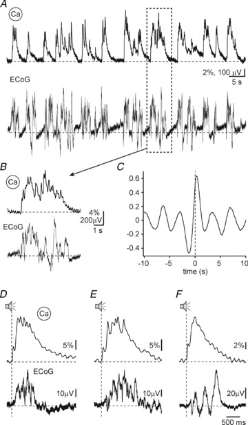
A, simultaneous recording of the calcium signal (upper panels) and the electrocorticogram (lower panels) during periods of spontaneous activity. B, magnified view of a network calcium transient and the simultaneously recorded ECoG. The traces are expanded from the recording section marked by a dashed square in A. C, cross-correlation between the spontaneous calcium signals and the ECoG shown in A. The cross-correlation has a peak with a positive delay, indicating that spontaneous calcium transients tend to follow the electrical signal. D–F, three examples of sound-evoked network calcium transients (upper panels) and the simultaneously recorded ECoG signals (lower panels). In these cases, the ECoG signal follows the population calcium signals.

During sound stimulation, the temporal relationship between the calcium transients and the epidural potentials changed. Instead of following the epidural potentials, the calcium transients now often preceded them (Fig. 6D–F). To study in more detail the sound-evoked NCaTs, the calcium signal at stimulus onset and the latency between stimulus onset and the following calcium transients were used to find 991 stimulus presentations that (1) occurred when the calcium signal was close to baseline, (2) during an epidural ‘down state’, and (3) elicited a calcium transient with a latency of less than 50 ms. In 925 out of these 991 cases (93%), an epidural ‘up state’ was initiated following the onset of the calcium transient, as in Fig. 6D–F. The mean latency to the epidural ‘up state’ was 325 ± 300 ms (mean ± SD), and the mode was 209 ms. These latencies were significantly shorter than the typical interval between epidural ‘up states’ (>1 s). Thus, sound-evoked early calcium transients typically initiated an epidural ‘up state’.

The slow network calcium transients are initiated by activity in layer 5 pyramidal neurons

In order to study the mechanisms underlying the initiation of slow NCaTs we used an optogenetic approach to directly stimulate a defined cortical layer. As layer 5 most probably contributes essentially to the initiation of slow NCaTs (Sanchez-Vives & McCormick, 2000; Sakata & Harris, 2009), we chose to investigate the Thy1-ChR2 transgenic mouse line which expresses the light-gated depolarizing channel channelrhodopsin-2 (ChR2) in layer 5 pyramidal neurons (Fig. 7A) (Arenkiel et al. 2007). Optogenetic stimulation reliably gave rise to calcium transients (Fig. 7B and C, right panels). These transients lacked the initial fast response component that we observed after sound stimulation (Fig. 7B and C, left panels). However, the structure of the ChR2-evoked transients was strikingly similar to that of the spontaneous and sound-evoked slow NCaTs (Fig. 7D; n = 253 sound-evoked, 213 spontaneous and 150 optogenetically evoked calcium transients; Mann–Whitney test; evoked-ChR2: rise time P = 0.11, FWHM P = 0.11, decay time constant P = 0.32; spontaneous-ChR2: rise time P = 0.62, FWHM P = 0.18, decay time constant P = 0.81). Thus, activation of layer 5 pyramidal neurons may play an important role in initiating the slow NCaTs, in contrast to the origin of the early component of the calcium transients, which is presumably due to the thalamo-cortical inputs. Moreover, this experiment demonstrates that the slow component of the calcium transients can be initiated intracortically, without direct thalamic contribution.

Figure 7. Optogenetic initiation of network calcium transients by activation of layer 5 pyramidal neurons.

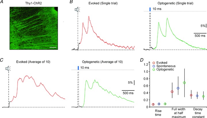
A, expression of channelrhodopsin-2 (ChR2) in layer 5 pyramidal neurons of the ChR2-Thy1 transgenic mouse line. Scale bar, 100 μm. B and C, single response (B) and average of 10 responses (C) to noise (left panels) and light stimulation (right panels). D, rise times, full widths at half-maximum and decay time constants of sound-evoked slow network calcium transients (red, n = 253 events from 10 animals), spontaneous network calcium transients (blue, n = 213 event from 10 animals) and optogenetically initiated network calcium transients (green, n = 159 events from 5 animals). All distributions are represented by the medians (circles) and interquartile ranges. Mann–Whitney test, evoked-ChR2: rise time P = 0.11, FWHM P = 0.11, decay time constant P = 32, spontaneous-ChR2: rise time P = 0.62, FWHM P = 0.18, decay time constant P = 0.81. Please note that only transients starting from the fluorescence baseline level were included in this analysis.

Discussion

This paper presents the first use of population calcium signals to study cortical dynamics and sensory responses in auditory cortex. While auditory-evoked calcium responses can be recorded at single cell (Bandyopadhyay et al. 2010; Rothschild et al. 2010) and subcellular levels (Chen et al. 2011), the study of population responses provides important information for understanding the large-scale dynamics of the brain (Harris et al. 2011). Here, we describe sound-evoked slow network calcium transients (NCaTs) which are essentially identical to spontaneous calcium transients, occur with a latency that is substantially longer than the one usually associated with sensory responses in auditory cortex, tend to be larger than the evoked short-latency responses, are strongly associated with global electrical ‘up states’ and can be elicited by optogenetic activation of layer 5 pyramidal neurons.

Origin of the NCaTs

NCaTs originate from both neurons and the neuropil. The volume from which NCaTs are recorded is illustrated in Fig. 1B: it has a width between 200 and 400 μm and a depth of 400–600 μm. Relating this to anatomical studies (e.g. Stiebler et al. 1997), we are recording from about 20% of the core auditory fields of the mouse auditory cortex. Thus, the recordings clearly cover only a small part of the tonotopic map in the mouse auditory cortex.

The calcium signal from neurons reflects the neuronal action potential firing whereas the signal recorded from the neuropil has been shown to represent calcium signals in axonal presynaptic structures (Stosiek et al. 2003; Kerr et al. 2005; Greenberg et al. 2008; Rochefort et al. 2009). Calcium signals from the dendritic structure, however, contribute little or nothing to the neuropil signal (Kerr et al. 2005). It is important to note that this is in contrast to the labelling of single cells using the whole-cell configuration or single-cell electroporation which makes it possible to record subthreshold dendritic and spine calcium transients (Jia et al. 2010; Chen et al. 2011). Astrocytic calcium transients do not play an essential role for NCaTs as their rate of occurrence and time course is markedly different from the one of the NCaTs. Using two-photon experiments we found that neurons and the neuropil are contributing about equally to NCaTs. In addition, we estimate that the activity of at least 20 active neurons in combination with the surrounding neuropil is required to generate NCaTs.

Comparison with other population signals

The NCaTs recorded by the optical fibre-based recording system are population calcium signals, and as such they should be compared with other indicators of population activity, such as intrinsic optical signals, multiunit responses, local field potentials (LFPs) and the signals obtained by voltage-sensitive dye (VSD) imaging.

The calcium signals are an indirect measure of electrical activity, as they are a consequence of the local network spiking activity (Kerr et al. 2005; Berger et al. 2007; Rochefort et al. 2009). Therefore, they are more specific than the intrinsic optical signals which reflect blood flow and therefore metabolic mechanisms that are farther downstream from the electrical activity (Grinvald et al. 1986). Voltage-sensitive dyes report electrical activity directly, but in contrast to the calcium signals, they are dominated by dendritic subthreshold signals, rather than by the spiking activity (Grinvald & Hildesheim, 2004). Thus, the calcium signals reflect the output of the neuronal population in ways that are impossible to achieve with voltage-sensitive dyes.

Although the calcium signals only indirectly reflect electrical activity, they have some advantages over LFP recordings. LFPs are believed to reflect synaptic responses rather than spiking activity. Furthermore, LFPs reflect activity that may occur far from the recording electrode as the LFP is integrated over a radius of at least 1 mm (Nelken & Ulanovsky, 2007), which is about the size of the whole mouse primary auditory cortex. In contrast, the data presented here suggest that the calcium signals can be recorded from limited extents of the tonotopic map. The width of tuning of the fast evoked components suggests that these calcium signals are due to the activity of populations that are about as large as electrically measured multiunit activity: indeed, the radius of the fibre is equal to the distance over which action potentials can be recorded from a neuron using a metal electrode (about 100 μm) (Abeles, 1982).

The two components of sound-evoked network calcium transients

The recordings of NCaTs in this study revealed two distinct components of sensory-evoked calcium responses in the auditory cortex: an early, fast-rising transient followed by a large, slow, long-latency calcium transient. The initial fast transient is missing in spontaneous and in optogenetically evoked calcium transients and is most probably due to thalamic afferents to lower layer 3, layer 4 and the layer 5/6 border (Romanski & LeDoux, 1993; Kimura et al. 2003; Winer & Lee, 2007). Interestingly, the two components of the sensory-evoked NCaT depended differently on the level of spontaneous activity at stimulus onset, represented by the fluorescence level at stimulus onset. The early transient was only weakly dependent, if at all, on the fluorescence level at stimulus onset. In contrast, the amplitude of the long-latency, slow NCaT depended strongly on the fluorescence level at stimulus onset. Thus, the two activity types, spontaneous and sensory-evoked slow NCaTs, essentially excluded each other. This suggests that the slow transient is probably produced by the same group of neurons that produces the spontaneous transients. Our two-photon calcium imaging experiments suggest that the population of neurons underlying the slow component is located throughout the cortical volume from which the fibre is recording (including layer 2/3). In fact, the slow sensory-evoked NCaT may be due to the non-synchronous small increases in the firing rate of this large population of neurons which is detectable partially in our two-photon experiments. An increase of even a few spikes in the firing of every neuron (due to the transition from a ‘down’ to an ‘up state’ which is linked to an increase in the probability for the firing of action potentials) would probably result in a substantial increase in fluorescence, as we observed in our optical fibre recordings.

Interestingly, optogenetic activation of layer 5 pyramidal neurons gave rise to very similar calcium transients. Thus, we can suggest a possible mechanism for the generation of the slow sensory-driven NCaTs: an incoming volley of activity from the thalamus evokes short-latency, synchronized activity in the thalamo-recipient layers of the cortex (which was not picked up in the two-photon imaging performed in layer 2/3). This activity propagates up to layer 2/3 and down to the infragranular layers, triggering an NCaT.

Several electrophysiological studies reported the presence of late, informative response components in different species in vitro and in vivo (Sally & Kelly, 1988; Metherate & Cruikshank, 1999; Wang et al. 2005; Moshitch et al. 2006; Sakata & Harris, 2009; Campbell et al. 2010). Metherate & Cruikshank (1999) described findings in an auditory thalamocortical slice preparation that are highly consistent with our results obtained in vivo using sensory stimulation. They report the presence of an electrical stimulation-evoked short-latency potential in layer IV, which was followed by a polysynaptic slow potential that propagated intracortically. Moshitch et al. (2006), when recording in the halothane-anaesthetized cat, found late spiking responses, lasting hundreds of milliseconds after stimulus offset, elicited by pure tone presentations. These responses were informative about tone frequency, and may have been related to the late NCaT. However, even in that study, stimulation rate was 1 Hz, limiting the ability to observe the full time course of the late activity. Similarly, Harris and collaborators used simultaneous recordings of multiple single neurons to demonstrate the presence of structured activity that could outlast sensory stimulation by a substantial amount of time (Bartho et al. 2009; Curto et al. 2009; Sakata & Harris, 2009). This sustained activity could be the electrical counterpart of the transients we measured. The electrical activity studied by Harris and collaborators was relatively weak in each specific neuron. Only by studying many neurons together could its properties be revealed. The use of population calcium signals puts this component of the evoked sensory responses in sharp relief.

Sound-evoked slow calcium transient and global ‘up states’

We found that the spontaneous and sensory-evoked slow NCaTs were strongly correlated with electrical slow waves that were present globally over large areas of the brain. These slow waves are tightly linked to slow oscillations of the membrane potential of single neurons from the hyperpolarized ‘down’ to the depolarized ‘up state’ and the ‘up state’ is associated with an increased probability of action potential firing (Steriade et al. 1993a,b). These slow oscillations seem to be initiated in vitro first in layer 5 pyramidal neurons (Sanchez-Vives & McCormick, 2000). Correspondingly, we found that calcium transients that were indistinguishable from spontaneous and sound-evoked slow calcium transients were elicited by activation of layer 5 pyramidal neurons. We therefore suggest that all three forms of activity – spontaneous, sound-evoked and optogenetically initiated slow transients – reflect a specific population mode, initiated in a cortical column by activation of layer 5 pyramidal neurons.

Studies performed in humans and other cortical areas of rodents suggest that electrically recorded slow waves may not be a local event, but in fact represent travelling waves, involving progressively more and more cortical areas (Massimini et al. 2004; Ferezou et al. 2007; Xu et al. 2007). In our study, the delays between the epidural signals and the spontaneous calcium signals recorded in the auditory cortex indicate that the generators of the spontaneous slow waves are not (or not exclusively) located within the auditory cortex. The spontaneous epidural ‘up states’ may be associated with the onset of activity in some other part of the cortex, which propagates to the auditory cortex and is detected there as a spontaneous calcium transient. In the same vein, after sound stimulation, a calcium transient elicited in the auditory cortex seems to initiate an epidural global ‘up state’ that may propagate across the brain as well. It is tempting to interpret in this way the presence of pure tone-evoked transients that lack the fast, early component. These transients may represent a propagating wave that was presumably generated at the cortical location whose best frequency corresponds to the stimulus, and was then propagated to the recording location. Under this assumption, it is possible to roughly estimate the speed of propagation of this wave: it covers a distance of about 1 mm (the rough size of a field in the mouse auditory cortex) in about 100 ms (the typical range of response onsets, as in Fig. 5C), suggesting that the propagation velocity of the wave is roughly 0.01 m s⁻¹. This velocity corresponds nicely with the measurements of Metherate & Cruikshank (1999) obtained in vitro, whose slow wave of activity propagated at a velocity of 0.02 m s⁻¹. The measurement of population calcium activity thus provides an intriguing window into the relationships between global and local forms of population activity in the brain and their role in neuronal processing.

Glossary

Abbreviations

A1

primary field

AAF

anterior auditory field

FWHM

full width at half-maximum

LFP

local field potential

NCaT

network calcium transients

VSD

voltage-sensitive dye

Author's present address

O. Garaschuk: Institute of Physiology II, Universität Tübingen, Keplerstr. 15, 72074 Tübingen, Germany.

Author contributions

C.G., H.A., R.-I.M., O.G., I.N. and A.K. designed the experiments. C.G., H.A., A.S., R.-I.M., O.G., A.S. and I.N. performed experiments. All authors analysed and interpreted the data. C.G., H.A., A.S., I.N. and A.K. wrote the manuscript. All authors approved the final version of the manuscript.

References

- Abeles M. Local Cortical Circuits: an Electrophysiological Study. Vol. 6. Berlin Heidelberg New York: Springer-Verlag; 1982. [Google Scholar]
- Adelsberger H, Garaschuk O, Konnerth A. Cortical calcium waves in resting newborn mice. Nat Neurosci. 2005;8:988–990. doi: 10.1038/nn1502. [DOI] [PubMed] [Google Scholar]
- Arenkiel BR, Peca J, Davison IG, Feliciano C, Deisseroth K, Augustine GJ, Ehlers MD, Feng G. In vivo light-induced activation of neural circuitry in transgenic mice expressing channelrhodopsin-2. Neuron. 2007;54:205–218. doi: 10.1016/j.neuron.2007.03.005. [DOI] [PMC free article] [PubMed] [Google Scholar]
- Badea T, Goldberg J, Mao B, Yuste R. Calcium imaging of epileptiform events with single-cell resolution. J Neurobiol. 2001;48:215–227. doi: 10.1002/neu.1052. [DOI] [PubMed] [Google Scholar]
- Bandyopadhyay S, Shamma SA, Kanold PO. Dichotomy of functional organization in the mouse auditory cortex. Nat Neurosci. 2010;13:361–368. doi: 10.1038/nn.2490. [DOI] [PMC free article] [PubMed] [Google Scholar]
- Bartho P, Curto C, Luczak A, Marguet SL, Harris KD. Population coding of tone stimuli in auditory cortex: dynamic rate vector analysis. Eur J Neurosci. 2009;30:1767–1778. doi: 10.1111/j.1460-9568.2009.06954.x. [DOI] [PMC free article] [PubMed] [Google Scholar]
- Berger T, Borgdorff A, Crochet S, Neubauer FB, Lefort S, Fauvet B, Ferezou I, Carleton A, Luscher H-R, Petersen CCH. Combined voltage and calcium epifluorescence imaging in vitro and in vivo reveals subthreshold and suprathreshold dynamics of mouse barrel cortex. J Neurophysiol. 2007;97:3751–3762. doi: 10.1152/jn.01178.2006. [DOI] [PubMed] [Google Scholar]
- Bullock TH. Signals and signs in the nervous system: The dynamic anatomy of electrical activity is probably information-rich. Proc Natl Acad Sci U S A. 1997;94:1–6. doi: 10.1073/pnas.94.1.1. [DOI] [PMC free article] [PubMed] [Google Scholar]
- Campbell RA, Schulz AL, King AJ, Schnupp JW. Brief sounds evoke prolonged responses in anesthetized ferret auditory cortex. J Neurophysiol. 2010;103:2783–2793. doi: 10.1152/jn.00730.2009. [DOI] [PMC free article] [PubMed] [Google Scholar]
- Castro-Alamancos MA. Dynamics of sensory thalamocortical synaptic networks during information processing states. Prog Neurobiol. 2004;74:213–247. doi: 10.1016/j.pneurobio.2004.09.002. [DOI] [PubMed] [Google Scholar]
- Chen X, Leischner U, Rochefort NL, Nelken I, Konnerth A. Functional mapping of single spines in cortical neurons in vivo. Nature. 2011;475:501–505. doi: 10.1038/nature10193. [DOI] [PubMed] [Google Scholar]
- Chervin RD, Pierce PA, Connors BW. Periodicity and directionality in the propagation of epileptiform discharges across neocortex. J Neurophysiol. 1988;60:1695–1713. doi: 10.1152/jn.1988.60.5.1695. [DOI] [PubMed] [Google Scholar]
- Crunelli V, Hughes SW. The slow (<1 Hz) rhythm of non-REM sleep: a dialogue between three cardinal oscillators. Nat Neurosci. 2010;13:9–17. doi: 10.1038/nn.2445. [DOI] [PMC free article] [PubMed] [Google Scholar]
- Curto C, Sakata S, Marguet S, Itskov V, Harris KD. A simple model of cortical dynamics explains variability and state dependence of sensory responses in urethane-anesthetized auditory cortex. J Neurosci. 2009;29:10600–10612. doi: 10.1523/JNEUROSCI.2053-09.2009. [DOI] [PMC free article] [PubMed] [Google Scholar]
- Doi A, Mizuno M, Katafuchi T, Furue H, Koga K, Yoshimura M. Slow oscillation of membrane currents mediated by glutamatergic inputs of rat somatosensory cortical neurons: in vivo patch-clamp analysis. Eur J Neurosci. 2007;26:2565–2575. doi: 10.1111/j.1460-9568.2007.05885.x. [DOI] [PubMed] [Google Scholar]
- Edeline J-M. The thalamo-cortical auditory receptive fields: regulation by the states of vigilance, learning and the neuromodulatory systems. Exp Brain Res. 2003;153:554–572. doi: 10.1007/s00221-003-1608-0. [DOI] [PubMed] [Google Scholar]
- Ehret G. Infant rodent ultrasounds – a gate to the understanding of sound communication. Behav Genet. 2005;35:19–29. doi: 10.1007/s10519-004-0853-8. [DOI] [PubMed] [Google Scholar]
- Engel AK, Fries P, Singer W. Dynamic predictions: Oscillations and synchrony in top-down processing. Nat Rev Neurosci. 2001;2:704–716. doi: 10.1038/35094565. [DOI] [PubMed] [Google Scholar]
- Engel AK, Singer W. Temporal binding and the neural correlates of sensory awareness. Trends in Cogn Sci. 2001;5:16–25. doi: 10.1016/s1364-6613(00)01568-0. [DOI] [PubMed] [Google Scholar]
- Ferezou I, Haiss F, Gentet LJ, Aronoff R, Weber B, Petersen CCH. Spatiotemporal dynamics of cortical sensorimotor integration in behaving mice. Neuron. 2007;56:907–923. doi: 10.1016/j.neuron.2007.10.007. [DOI] [PubMed] [Google Scholar]
- Fernald RD, Gerstein GL. Response of cat cochlear nucleus neurons to frequency and amplitude modulated tones. Brain Res. 1972;45:417–435. doi: 10.1016/0006-8993(72)90472-6. [DOI] [PubMed] [Google Scholar]
- Garaschuk O, Milos RI, Grienberger C, Marandi N, Adelsberger H, Konnerth A. Optical monitoring of brain function in vivo: from neurons to networks. Pflugers Arch. 2006a;453:385–396. doi: 10.1007/s00424-006-0150-x. [DOI] [PubMed] [Google Scholar]
- Garaschuk O, Milos RI, Konnerth A. Targeted bulk-loading of fluorescent indicators for two-photon brain imaging in vivo. Nat Protoc. 2006b;1:380–386. doi: 10.1038/nprot.2006.58. [DOI] [PubMed] [Google Scholar]
- Greenberg DS, Houweling AR, Kerr JND. Population imaging of ongoing neuronal activity in the visual cortex of awake rats. Nat Neurosci. 2008;11:749–751. doi: 10.1038/nn.2140. [DOI] [PubMed] [Google Scholar]
- Grinvald A, Hildesheim R. VSDI: a new era in functional imaging of cortical dynamics. Nat Rev Neurosci. 2004;5:874–885. doi: 10.1038/nrn1536. [DOI] [PubMed] [Google Scholar]
- Grinvald A, Lieke E, Frostig RD, Gilbert CD, Wiesel TN. Functional architecture of cortex revealed by optical imaging of intrinsic signals. Nature. 1986;324:361–364. doi: 10.1038/324361a0. [DOI] [PubMed] [Google Scholar]
- Harris KD, Bartho P, Chadderton P, Curto C, de la Rocha J, Hollender L, Itskov V, Luczak A, Marguet SL, Renart A, Sakata S. How do neurons work together? Lessons from auditory cortex. Hear Res. 2011;271:37–53. doi: 10.1016/j.heares.2010.06.006. [DOI] [PMC free article] [PubMed] [Google Scholar]
- Holy TE, Guo Z. Ultrasonic songs of male mice. PLoS Biol. 2005;3:e386. doi: 10.1371/journal.pbio.0030386. [DOI] [PMC free article] [PubMed] [Google Scholar]
- Hromadka T, Deweese MR, Zador AM. Sparse representation of sounds in the unanesthetized auditory cortex. PLoS Biol. 2008;6:e16. doi: 10.1371/journal.pbio.0060016. [DOI] [PMC free article] [PubMed] [Google Scholar]
- Jia H, Rochefort NL, Chen X, Konnerth A. Dendritic organization of sensory input to cortical neurons in vivo. Nature. 2010;464:1307–1312. doi: 10.1038/nature08947. [DOI] [PubMed] [Google Scholar]
- Kerr JN, Greenberg D, Helmchen F. Imaging input and output of neocortical networks in vivo. Proc Natl Acad Sci U S A. 2005;102:14063–14068. doi: 10.1073/pnas.0506029102. [DOI] [PMC free article] [PubMed] [Google Scholar]
- Kimura A, Donishi T, Sakoda T, Hazama M, Tamai Y. Auditory thalamic nuclei projections to the temporal cortex in the rat. Neuroscience. 2003;117:1003–1016. doi: 10.1016/s0306-4522(02)00949-1. [DOI] [PubMed] [Google Scholar]
- Kisley MA, Gerstein GL. Trial-to-trial variability and state-dependent modulation of auditory-evoked responses in cortex. J Neurosci. 1999;19:10451–10460. doi: 10.1523/JNEUROSCI.19-23-10451.1999. [DOI] [PMC free article] [PubMed] [Google Scholar]
- Linden JF, Liu RC, Sahani M, Schreiner CE, Merzenich MM. Spectrotemporal structure of receptive fields in areas AI and AAF of mouse auditory cortex. J Neurophysiol. 2003;90:2660–2675. doi: 10.1152/jn.00751.2002. [DOI] [PubMed] [Google Scholar]
- Lütcke H, Murayama M, Hahn T, Margolis DJ, Astori S, Zum Alten Borgloh SM, Gobel W, Yang Y, Tang W, Kugler S, Sprengel R, Nagai T, Miyawaki A, Larkum ME, Helmchen F, Hasan MT. Optical recording of neuronal activity with a genetically-encoded calcium indicator in anesthetized and freely moving mice. Front Neural Circuits. 2010;4:9. doi: 10.3389/fncir.2010.00009. [DOI] [PMC free article] [PubMed] [Google Scholar]
- Marguet SL, Harris KD. State-dependent representation of amplitude-modulated noise stimuli in rat auditory cortex. J Neurosci. 2011;31:6414–6420. doi: 10.1523/JNEUROSCI.5773-10.2011. [DOI] [PMC free article] [PubMed] [Google Scholar]
- Massimini M, Huber R, Ferrarelli F, Hill S, Tononi G. The sleep slow oscillation as a traveling wave. J Neurosci. 2004;24:6862–6870. doi: 10.1523/JNEUROSCI.1318-04.2004. [DOI] [PMC free article] [PubMed] [Google Scholar]
- Metherate R, Cruikshank SJ. Thalamocortical inputs trigger a propagating envelope of gamma-band activity in auditory cortex in vitro. Exp Brain Res. 1999;126:160–174. doi: 10.1007/s002210050726. [DOI] [PubMed] [Google Scholar]
- Moshitch D, Las L, Ulanovsky N, Bar-Yosef O, Nelken I. Responses of neurons in primary auditory cortex (A1) to pure tones in the halothane-anesthetized cat. J Neurophysiol. 2006;95:3756–3769. doi: 10.1152/jn.00822.2005. [DOI] [PubMed] [Google Scholar]
- Nelken I, Ulanovsky N. Change detection, mismatch negativity and stimulus-specific adaptation in animal models. J Psychophysiol. 2007;21:214–223. [Google Scholar]
- Nimmerjahn A, Kirchhoff F, Kerr JN, Helmchen F. Sulforhodamine 101 as a specific marker of astroglia in the neocortex in vivo. Nat Methods. 2004;1:31–37. doi: 10.1038/nmeth706. [DOI] [PubMed] [Google Scholar]
- Pesaran B, Pezaris JS, Sahani M, Mitra PP, Andersen RA. Temporal structure in neuronal activity during working memory in macaque parietal cortex. Nat Neurosci. 2002;5:805–811. doi: 10.1038/nn890. [DOI] [PubMed] [Google Scholar]
- Petersen CC, Hahn TT, Mehta M, Grinvald A, Sakmann B. Interaction of sensory responses with spontaneous depolarization in layer 2/3 barrel cortex. Proc Natl Acad Sci U S A. 2003;100:13638–13643. doi: 10.1073/pnas.2235811100. [DOI] [PMC free article] [PubMed] [Google Scholar]
- Rochefort NL, Garaschuk O, Milos RI, Narushima M, Marandi N, Pichler B, Kovalchuk Y, Konnerth A. Sparsification of neuronal activity in the visual cortex at eye-opening. Proc Natl Acad Sci U S A. 2009;106:15049–15054. doi: 10.1073/pnas.0907660106. [DOI] [PMC free article] [PubMed] [Google Scholar]
- Romanski LM, LeDoux JE. Organization of rodent auditory cortex: anterograde transport of PHA-L from MGv to temporal neocortex. Cereb Cortex. 1993;3:499–514. doi: 10.1093/cercor/3.6.499. [DOI] [PubMed] [Google Scholar]
- Rothschild G, Nelken I, Mizrahi A. Functional organization and population dynamics in the mouse primary auditory cortex. Nat Neurosci. 2010;13:353–360. doi: 10.1038/nn.2484. [DOI] [PubMed] [Google Scholar]
- Sachdev RN, Ebner FF, Wilson CJ. Effect of subthreshold up and down states on the whisker-evoked response in somatosensory cortex. J Neurophysiol. 2004;92:3511–3521. doi: 10.1152/jn.00347.2004. [DOI] [PubMed] [Google Scholar]
- Sakata S, Harris KD. Laminar structure of spontaneous and sensory-evoked population activity in auditory cortex. Neuron. 2009;64:404–418. doi: 10.1016/j.neuron.2009.09.020. [DOI] [PMC free article] [PubMed] [Google Scholar]
- Sally SL, Kelly JB. Organization of auditory cortex in the albino rat: sound frequency. J Neurophysiol. 1988;59:1627–1638. doi: 10.1152/jn.1988.59.5.1627. [DOI] [PubMed] [Google Scholar]
- Sanchez-Vives MV, McCormick DA. Cellular and network mechanisms of rhythmic recurrent activity in neocortex. Nat Neurosci. 2000;3:1027–1034. doi: 10.1038/79848. [DOI] [PubMed] [Google Scholar]
- Sanderson MJ, Parker I. Video-rate confocal microscopy. Methods Enzymol. 2003;360:447–481. doi: 10.1016/s0076-6879(03)60123-0. [DOI] [PubMed] [Google Scholar]
- Schroeder CE, Tenke CE, Givre SJ, Arezzo JC, Vaughan HG., Jr Laminar analysis of bicuculline-induced epileptiform activity in area 17 of the awake macaque. Brain Res. 1990;515:326–330. doi: 10.1016/0006-8993(90)90617-k. [DOI] [PubMed] [Google Scholar]
- Steriade M, Nunez A, Amzica F. A novel slow (<1 Hz) oscillation of neocortical neurons in vivo: depolarizing and hyperpolarizing components. J Neurosci. 1993a;13:3252–3265. doi: 10.1523/JNEUROSCI.13-08-03252.1993. [DOI] [PMC free article] [PubMed] [Google Scholar]
- Steriade M, Nunez A, Amzica F. Intracellular analysis of relations between the slow (<1 Hz) neocortical oscillation and other sleep rhythms of the electroencephalogram. J Neurosci. 1993b;13:3266–3283. doi: 10.1523/JNEUROSCI.13-08-03266.1993. [DOI] [PMC free article] [PubMed] [Google Scholar]
- Stiebler I, Neulist R, Fichtel I, Ehret G. The auditory cortex of the house mouse: left-right differences, tonotopic organization and quantitative analysis of frequency representation. J Comp Physiol A. 1997;181:559–571. doi: 10.1007/s003590050140. [DOI] [PubMed] [Google Scholar]
- Stosiek C, Garaschuk O, Holthoff K, Konnerth A. In vivo two-photon calcium imaging of neuronal networks. Proc Natl Acad Sci U S A. 2003;100:7319–7324. doi: 10.1073/pnas.1232232100. [DOI] [PMC free article] [PubMed] [Google Scholar]
- Turner JG, Parrish JL, Hughes LF, Toth LA, Caspary DM. Hearing in laboratory animals: strain differences and nonauditory effects of noise. Comp Med. 2005;55:12–23. [PMC free article] [PubMed] [Google Scholar]
- Wang X, Lu T, Snider RK, Liang L. Sustained firing in auditory cortex evoked by preferred stimuli. Nature. 2005;435:341–346. doi: 10.1038/nature03565. [DOI] [PubMed] [Google Scholar]
- Winer JA, Lee CC. The distributed auditory cortex. Hear Res. 2007;229:3–13. doi: 10.1016/j.heares.2007.01.017. [DOI] [PMC free article] [PubMed] [Google Scholar]
- Worgotter F, Suder K, Zhao Y, Kerscher N, Eysel UT, Funke K. State-dependent receptive-field restructuring in the visual cortex. Nature. 1998;396:165–168. doi: 10.1038/24157. [DOI] [PubMed] [Google Scholar]
- Xu W, Huang X, Takagaki K, Wu J-Y. Compression and reflection of visually evoked cortical waves. Neuron. 2007;55:119–129. doi: 10.1016/j.neuron.2007.06.016. [DOI] [PMC free article] [PubMed] [Google Scholar]