Hydrophobic forces and the length limit of foldable protein domains

Abstract

To find the native conformation (fold), proteins sample a subspace that is typically hundreds of orders of magnitude smaller than their full conformational space. Whether such fast folding is intrinsic or the result of natural selection, and what is the longest foldable protein, are open questions. Here, we derive the average conformational degeneracy of a lattice polypeptide chain in water and quantitatively show that the constraints associated with hydrophobic forces are themselves sufficient to reduce the effective conformational space to a size compatible with the folding of proteins up to approximately 200 amino acids long within a biologically reasonable amount of time. This size range is in general agreement with the experimental protein domain length distribution obtained from approximately 1,200 proteins. Molecular dynamics simulations of the Trp-cage protein confirm this picture on the free energy landscape. Our analytical and computational results are consistent with a model in which the length and time scales of protein folding, as well as the modular nature of large proteins, are dictated primarily by inherent physical forces, whereas natural selection determines the native state.

Ever since the discovery that proteins can spontaneously self-assemble into unique three-dimensional shapes (folds) (1), the mechanism of this folding process has been a focus of biology. It has been shown that random sequences can fold into a unique ground state which is separated from other folds by an energy gap (2). However, assuming the existence of a unique native fold, there is no assurance that the protein can efficiently parse the fold space to find it. In particular, how nature is able to search the exponentially increasing number of folds accessible to proteins of nontrivial length has not been explicitly elucidated; Levinthal famously estimated that for a protein consisting of 150 amino acids, in which each degree of freedom is discretized into only ten possible values, it would take much longer than the age of the universe to sample all the folds even at the limit of molecular motion (3).

The qualitative resolution of the Levinthal paradox has been the concept of the folding funnel, whereby a global bias in the multidimensional energy landscape channels the protein toward the subspace containing the native fold (4). For example, by introducing an artificial search bias in favor of native contacts (5) or designing sequences favoring specific secondary structures (6), fast folding was computationally observed. This suggests that the funnel arises from evolutionary tuning of the intramolecular interactions via sequence mutation and that feasible protein folding times are the result of natural selection.

In contrast to this picture, we show below that a general effect, namely the hydrophobic force, is sufficient to account for the kinetics of fast folding without sequence evolution. This force, which is the global tendency for the chain to collapse to a compact shape and for the residues to segregate in the interior of proteins, has long been recognized as a dominant factor in protein folding (7, 8). Indeed, proteins have been experimentally (9, 10) and computationally (11) shown to undergo hydrophobic collapse in the earliest stage of folding. By considering the degeneracy of all folds, we demonstrate that hydrophobic collapse together with hydrophobic/hydrophilic residue segregation lead to realistic folding time scales for globular proteins and protein domains, which are independently folding subunits that constitute larger proteins (12), thus quantitatively resolving the paradox. We also find an upper limit, of approximately 200 amino acids, on the length of protein domains for which such hydrophobic packing constraints would allow the native state to be identified within a biologically reasonable timescale through a hypothetical exhaustive search. By comparing to the experimental distribution of protein domain lengths, we find that most protein fall below this “hydrophobic length limit,” although it can be exceeded due to the influence of other processes, besides the hydrophobic force, that affect protein folding.

Many attempts have been made to estimate the reduction of the effective search space due to the hydrophobic force. For a self-avoiding chain (SAC) composed of L residues on a three-dimensional cubic lattice, the number of unique conformational folds (degeneracy) was found to be N_SAC ∼ 4.68^L (13); if we further restrict the chain to adopt maximally compact folds, as defined in the mean field treatment (14), the degeneracy N_Compact = (6/e)^L, where e is the base of the natural logarithm. Although compaction significantly reduces the search space, and is a driving factor for secondary structure formation (15), the degeneracy is still astronomically large even for the smallest proteins.

The final step is the further reduction of the fold space by choosing only those compact folds with hydrophobic residues (H) maximally segregated, in the sense of maximizing the number of H-H contacts, into the interior of the protein, and polar residues (P) on the outside. This minimalist HP representation of proteins has been a mainstay of analytic investigations of protein folding (16). We define N_HP(s) to be the degeneracy of self-avoiding compact folds with maximum H/P segregation, which is a function of s, the sequence of H and P residues along the chain. Because hydrophobic residues are empirically randomly distributed along the protein sequence (17), the average conformational degeneracy of a collapsed H/P-segregated protein, , is equal to N_HP(s) averaged over all possible s of length L, where “” denotes averaging over the sequence space. Therefore, represents the size of the effective fold space, on average, when a protein folds in a polar solvent like water.

The chief difficulty in obtaining is the constraint that all monomers must be connected in a chain; this constraint had made N_HP(s) impossible to analytically compute for any given sequence s, much less averaged over all s. Estimates that neglect to enforce the linear sequence of the chain, for example by assigning independent probabilities for each hydrophobic residue to be in the interior of the protein, overlook the crucial role of this constraint in reducing the degeneracy. Consequently, was found to grow almost as quickly as N_Compact as a function of L (16), and is nine orders of magnitude too large for L = 100 (see Results).

Alternatively, computational efforts have been made in order to explicitly account for chain connectivity. In two dimensions, Camacho et al computed by enumerating all such folds for all sequence permutations for L < 28, assuming that half the residues are H and half P (18). On a 2D lattice, was found to grow at a (sub)logarithmic rate and plateau at L ∼ 10. However, due to the exponentially growing number of both folds and sequences with increasing L, this process becomes computationally intractable for longer sequences. Crucially, the computational limit is even more severe in three dimensions, so that the description of 3D folding was extrapolated from 2D simulations (19). Indeed, it was found via explicit calculation for a random sampling of HP sequences of length 48 that N_HP(s) on a cubic lattice ranged from “thousands to millions” (20) which is incompatible with a logarithmic growth rate. Below, we analytically calculate in three dimensions, taking into account, unlike previous work, the fact that the residues on the lattice must be interconnected to form a chain. In this work, the chain length L is the only parameter of the solution obtained.

Results and Discussion

Lattice Model.

All calculations ignore prefactors of order unity. We define a map to be a spatial arrangement of H and P residues. In the HP model, each H–H contact in the map decreases the energy by a fixed amount, whereas all other contacts do not contribute energetically. For a particular sequence s of length L, N_HP(s) technically describes the number of folds of sequence s that achieve the optimal (i.e., lowest energy) map for that sequence. This may not be the same as the optimal map over all sequences of length L, which we call the global optimal map. We define 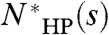as the number of folds that achieve the global optimal map. If s can achieve the global optimal map, then 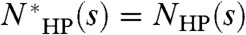, otherwise . Hence, is a lower bound on . If 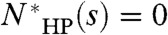, then N_HP(s) is bounded by the probability that none of the optimal folds of s can be locally perturbed to achieve lower energy maps. Consequently, in three dimensions, the sequences that cannot achieve the global optimal map do not contribute significantly to , hence (see Methods).

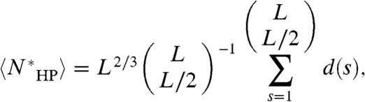
To calculate , consider the sequence-versus-fold space for an L-residue protein (Fig. 1). Each column corresponds to a unique sequence, and each row corresponds to a unique compact fold. Since the ratio of polar to hydrophobic residues in proteins is 1∶1 (21), there are columns and (6/e)^L rows (i.e., N_Compact). Fig. 1 schematically illustrates this table for L = 36 on a two-dimensional lattice for clarity, although the concept is identical in three dimensions. Thus,

[1]

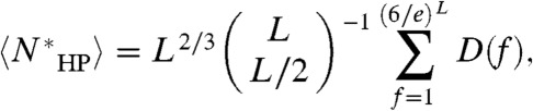
where d(s) is number of folds for which sequence s achieves a global optimal map, and the prefactor L^2/3 accounts for the number of distinct global optimal maps due to the possible locations along the H-surface to place leftover H residues (unless the number of H residues is a perfect cube). All relevant constraints, including chain connectivity, are captured by d(s). Summing the row (fold) degeneracy of the global optimal map over all columns (sequences) is equivalent to summing the column (sequence) degeneracy over all rows (folds). Therefore,

[2]

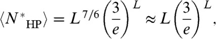
where D(f) is the sequence degeneracy of fold f. For any map, a given sequence can achieve the map via multiple (or no) folds; on the contrary, any fold can achieve any map with exactly one sequence: D(f) = 1 for all f. Thus, . Applying Stirling’s approximation, we obtain the following main results. The degeneracy is given by:

[3]

and the folding time for exhaustive search is simply:

[4]

where τ_sampling is the time it takes the chain to change from one conformation to another. We note that these results are for a 3D lattice. In two dimensions, (3/e)^L becomes (2/e)^L, which is an exponentially decreasing function; although the prefactor L^7/6 and τ_sampling depend on the number of dimensions, they are not the determining factors as L increases. In this 2D case, longer chains will have a diminishing probability of folding into the global optimal map; as L increases, the chain continuously “runs out” of ways to fold to the optimal map, and maps of increasing energy will become optimal. This turnover of the optimal map causes , the optimal map degeneracy, to plateau as a function of L, in agreement with the explicit 2D calculations of Ref. (18).

Fig. 1.

Folds versus sequences on a lattice. White and black circles denote hydrophobic (H) and polar (P) residues, respectively. Each pattern of H and P circles constitutes a map. For any given map, a fixed sequence (e.g., column 1) can have multiple (or no) conformations which produce the same map (e.g., rows 1 and 2). On the other hand, each conformation (row) has one and only one sequence that can produces any map. For clarity, two-dimensional lattices are depicted; nevertheless, the results mainly pertain to three-dimensional lattices which are descriptive of protein folds.

Eq. 3 also correctly predicts lattice simulations in three dimensions. Consistent with the “thousands to millions” of degenerate optimal conformations estimated from explicit enumeration, 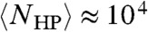for L = 48. At a higher level of chemical accuracy, for a L = 80 lattice chain consisting of the 20 types of amino acids and with a unique native fold, it was found that at most 10⁶ Monte Carlo steps were required to reach the native fold (22). This is in agreement with Eq. 3: 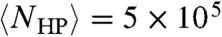for L = 80.

Multiplying by the experimentally determined 10-ns conformational rearrangement time (τ_sampling) (23), Eq. 4 converts the degeneracy into the folding time τ_folding. Fig. 2 (Top) plots the folding (or sampling) time of the self-avoiding chain N_SAC, compact self-avoiding chain N_Compact, and the average collapsed H/P-segregated chain as a function of L in three dimensions. In accordance with Levinthal, the number of conformations, even if restricted to the compact subset, becomes astronomically large for very short chains (N_SAC and N_Compact). Nevertheless, if confined to by hydrophobic segregation, exhaustive search of this subspace can be accomplished in biological time (nanoseconds to minutes) for L < 200. Because grows exponentially with L, beyond this length proteins cannot complete an exhaustive search of the hydrophobic subspace; this is the exhaustive hydrophobic search length limit for protein domains.

Fig. 2.

Hydrophobic length and folding time limits of folding. Degeneracy of conformations on a cubic lattice is plotted as a function of chain length (Top). Conformational degeneracies of self-avoiding chain (SAC), self-avoiding compact chain, and the sequence-averaged lowest energy HP chain are shown with dotted, dashed, and solid lines, respectively. The degeneracies are multiplied by the 10-ns residue reorganization time to obtain the exhaustive folding times. The predicted limit (above which folding cannot occur at biologically relevant timescales) is L ∼ 200 amino acids. Experimentally measured folding times taken from refs. 24 and 25 are also shown, indicating that faster-than-exhaustive-search folding occurs for L > 100. The experimental domain length distribution of a representative set of 1236 proteins (data from ref. (26)) shows that for L > 100, the population fraction begins to decay (Bottom). The protein populations are divided into the HP-dominated regime for L below the exhaustive search length limit (red arrow), and the natural selection (NS)-dominated regime for L above the length limit (green arrow). See text for further description of the regimes.

Also shown in Fig. 2 (Top) are the experimentally measured folding times for 65 single domain proteins (24, 25). For L < 100, the folding time agrees with the exhaustive sequence-averaged folding time τ_folding, with the variance arising from the particular protein sequence. For L > 100, the average folding time falls below τ_folding, indicating the onset of other factors such as sequence selection in order to evolve faster kinetics, despite the overall folding timescale for L < 200 being dominated by the H/P collapse.

Although proteins often consist of more than 1,000 amino acids, protein domains are on average 100 amino acids long, typically ranging from 50 to 200 (26, 27), with 90% being less than 200 (28), which we have established as the length regime for which hydrophobic-polar interactions are sufficient for fast folding (HP-dominated). Besides being composed of sequences with smaller degeneracy than that of the average sequence, or whose energy landscapes allow fast folding due to other forces besides hydrophobic force, longer domains often consist of periodic local structures as a result of repeat insertion mutations (29), and molecular chaperones can also assist in folding (30). These types of evolutionary selection allow for the existence of domains that exceed the hydrophobic length limit; the fast folding of proteins in this second regime is therefore consistent with the effect of natural selection (NS-dominated). Fig. 2 (Bottom) shows the domain length distribution of a representative sample of 1236 proteins (21) and its partitioning into the two regimes. Consistent with the folding data of Fig. 2 (Top), the population fraction of proteins with length L begins to decay near L = 100, consistent with the onset of evolutionary pressure at this length scale to select for sequences that fold faster than exhaustive search. However, since the folding degeneracy increases exponentially with L, the fraction of protein domains exceeding the L = 200 hydrophobic length limit is small. This may have forced most proteins with L > 200 to evolve as modular combinations of smaller domains.

Computational.

To complement the general, yet coarse-grained, results above, we also performed ensemble-convergent molecular dynamics (MD) simulations using the CHARMM suite of programs and force field (31) on a single polypeptide to gain insight at the atomistic level. We chose the 20-residue Trp-cage (32), which despite its small size contains both secondary and tertiary structure, in particular the burial of the large hydrophobic tryptophan side-chain in the interior. Vacuum phase simulations were performed for 76 independent trajectories, each lasting 2 µm. Solution phase simulations were performed explicitly represented solvent for 38 independent trajectories, each lasting 60 ns. All simulations were coupled to a Nose thermostat set at 28 °C to ensure a canonical room temperature ensemble, and the simulation time was long enough such that doubling of the simulation time did not significantly affect the results.

Fig. 3 shows the free energy landscape in both environments as a function of rmsd, the root-mean-squared deviation from the original experimentally determined structure and the solvent accessible surface area of the hydrophobic residues (exposed H area). In water, the peptide is confined to a free energy basin with burial of hydrophobic residues, including tryptophan (low exposed H area) and structure similar to that found experimentally (low rmsd). In the absence of water, the hydrophobic residues are more solvent-exposed; there are multiple conformational basins distributed throughout the free energy landscape, with some minima corresponding to predicted “inside-out” conformational ensembles (33), in which the hydrophobic residues are on the outside and the polar residues are buried. The polypeptide does not spend the majority of its time in the lowest free energy basin. Significantly, in accordance with the lattice model, the fold space is greatly diminished in water because the peptide is restricted to folds with buried hydrophobic residues.

Fig. 3.

Free energy landscapes of Trp-cage in the presence and absence of water from molecular dynamics simulations. White and black denote hydrophobic (H), and polar (P) residues, respectively. The two order parameters are rmsd from the experimentally determined starting structure and the solvent accessible surface area of the hydrophobic side chains (exposed H area). When solvated (Top), the landscape is restricted to the basin containing the native state; in vacuum (Bottom), there are a multitude of minima, all with similar free energies, that are no longer constrained to minimize the exposed H area. Some representative structures are also shown, including an “inside-out” conformation sampled during the vacuum simulations.

Because Trp-cage is unique, with its hydrophobic “core” primarily consisting of a single residue, care must be made when extrapolating specific dynamical behaviors to proteins in general. However, as a minimal-size peptide with tertiary structure for which comprehensive and statistically significant information can be obtained with atomic resolution, Trp-cage further confirms that the lattice results extend to the physical world.

Concluding Remarks

In this contribution, we addressed the apparent paradox of overwhelming fold degeneracy in protein folding, a problem that is analogous to the question of how proteins and genes evolve by natural selection within the immense space of possible sequences (34). Smith argued that the latter paradox vanishes if incremental evolutionary steps confine the protein sequence within the exponentially smaller sequence subspace that corresponds to good fitness (35). Just like evolutionary fitness is a global order parameter that keeps the sequence search within the fruitful subspace of all sequences, hydrophobic–hydrophobic contact area is a global order parameter that keeps the fold search within the fruitful subspace of folds. Here, we quantitatively demonstrate that the size of the subspace is indeed small enough to be realistically sampled over the course of protein folding.

The coarse-grained lattice has been used to derive the hydrophobic length limit of protein domains at approximately 200. In the regime below this length, proteins could in principle randomly sample the entire folding subspace consistent with hydrophobic collapse and hydrophobic/hydrophilic segregation. Above this length, the hydrophobically constrained fold space increases exponentially beyond what is accessible by random search. Consequently, the evolution of larger proteins is consistent with the model of modular growth, involving the aggregation, swapping, and duplication of stable domains (36). In this latter regime, natural selection may be necessary to enhance the folding rate using sequence-specificity and/or chaperones. The all-atom simulations explicitly demonstrate the role of the hydrophobic force in drastically reducing the search space on the free energy landscape.

In addition to providing a mechanistic insight into the role of physical forces in shaping the length-scale and evolution of proteins, the results presented here may be useful in protein characterization and engineering. For example, a useful metric that quantifies the effect of protein sequence on folding speed is the ratio of a protein’s folding time to τ_folding, the exhaustive search time of an average HP chain. In the case of protein design, we predict that for L < 200 it is not necessary to engineer a kinetic pathway which leads to the desired native state; as long as the native state is thermodynamically stable and the roughness of the folding energy landscape is sufficiently low, the protein will fold in a reasonable time.

Methods

Lattice Model.

We denote a sequence “optimal” if it can achieve the global optimal map, and “suboptimal” otherwise. We define p to be the fraction of sequences that can only fold into suboptimal maps, to be the average ground state degeneracy over all such suboptimal sequences, and the average ground state degeneracy over all optimal sequences. To show that , we note that ; it is therefore sufficient to show that . To this end, note that if a sequence is suboptimal, there exist lower energy states that it cannot achieve by locally perturbing any of its ground state folds. Being a globally suboptimal sequence, each ground state fold f of the sequence s contains a minimal-sized subvolume n(f,s) of the lattice in which the number of H–H contacts can be increased (and thus the energy decreased) by changing the positions of H and P residues to form a new map with lower energy in the subvolume. For each ground state fold f, assuming that there exists at least one other fold besides the starting fold which preserves the chain connectivity to the outside of the subvolume, define P_f to be the probability that at least one such fold can achieve a lower energy. Then, the probability that each residue of n(f,s) matches that of the lower-energy map is (1/2)^n(f,s). Therefore, P_f > (1/2)^n(f,s), where the greater-than sign is due to the possibility of multiple conformations, multiple lower energy maps, and unequal numbers of H and P residues within the subvolume which can all increase this probability. Then, the probability that none of the ground state folds can be locally perturbed to achieve a lower energy is:

[5]

where is the average size of the minimal volume over all sequences and over all ground state folds of each sequence. The approximation in Eq. 5 is justified because P_fN_S < 1/2 at the locally optimal fold. Since probabilities must be non-negative, we obtain from Eq. 5 that .

We can estimate by noting that there are three generic types of H-P swapping to achieve lower energy. First, there is the most likely case in which at least one extra H–H contact can be made by rearranging one surface of an H-region. The volume n(f,s) is therefore a path on an H-surface such that the H residue(s) at one end of the path swaps with the P residue(s) at the other end; the volume is thus at most twice the length of the cubic lattice: n(f,s) < 2L^1/3 (see Fig. 4, Top) for any fold f and sequence s.

Fig. 4.

Minimal subvolume required for H/P swapping leading to lower energy. The schematic illustrates the three types of swapping for a cubic lattice of length 6. The hydrophobic residues (H) are shown in gray and the hydrophilic residues (P) are transparent for clarity purposes. The individual gray cubes denote the hydrophobic portion of the minimal subvolume n. The three types are (Top) swapping on one face, (Center) swapping involving multiple faces, and (Bottom) merging distinct hydrophobic regions. Note that the schematic illustrates the extreme cases in each of the three swapping categories; most configurations require smaller distortions.

In the second case, rearrangement may require multiple H residues on one face of an H-region to swap with P residues on a different face. In this case (see Fig. 4, Center) the maximum n is limited to the area of a face : n(f,s) < L^2/3 for any fold f and sequence s.

Finally, there is the case which requires two separate H-regions to connect. In this case, all H-regions must be cubes, otherwise case 1 or case 2 would apply. The maximum n(f,s) corresponds to the case in which the lattice is divided into a three-dimensional checkerboard, with each H-region being a cube of sides at most L^1/3/2. Thus, the maximum n(f,s) is equal to this cube plus one face of the adjacent cube, so that the cube may be shifted by one and thereby make contact with another cube: n(f,s) < (L^1/3/2)² ∗ (L^1/3/2 + 1) = L/8 + L^2/3/4 (see Fig. 4, Bottom) for any fold f and sequence s.

In all three cases, for any fold f and sequence s. Since this is true for any f and s, it is true when n(f,s) is averaged over all f and s: . For example, for L = 200, , whereas 2ⁿ < 10⁵, 10¹⁰, and 10¹⁰ for (the worst-case scenarios of) the three cases, respectively. Therefore, , and thus .

MD Simulations.

The solution phase simulations were performed on the peptide, 3914 TIP3P (37) water molecules, and one chlorine atom for neutrality. The system was restricted to a cubic box with initial sides of 50 Å and equilibrated at constant temperature (298 K) and pressure (1 atm) with periodic boundary conditions. The trajectories were seeded from the 38 NMR structural variants. In the case of vacuum simulations, 1-ns solution phase simulations were performed on each of the 38 initial structures, and the final conformations from these simulations were used to double the number of trajectories. We also performed the vacuum-phase simulations without coupling to a thermal bath (microcanonical ensemble) and confirmed that the free energy landscape is not significantly affected.

References

- 1.Anfinsen CB. Principles that govern the folding of protein chains. Science. 1973;181:223–230. doi: 10.1126/science.181.4096.223. [DOI] [PubMed] [Google Scholar]
- 2.Shakhnovich EI, Gutin AM. Implications of thermodynamics of protein folding for evolution of primary sequences. Nature. 1990;346:773–775. doi: 10.1038/346773a0. [DOI] [PubMed] [Google Scholar]
- 3.Levinthal C. In: Mossbauer Spectroscopy in Biological Systems. Debrunner P, Tsibris JCM, Munck E, editors. Urbana: University of Illinois Press; 1969. pp. 22–24. [Google Scholar]
- 4.Frauenfelder H, Sligar SG, Wolynes PG. The energy landscapes and motions of proteins. Science. 1991;254:1598–1603. doi: 10.1126/science.1749933. [DOI] [PubMed] [Google Scholar]
- 5.Zwanzig R, Szabo A, Bagchi B. Levinthal’s paradox. Proc Natl Acad Sci USA. 1992;89:20–22. doi: 10.1073/pnas.89.1.20. [DOI] [PMC free article] [PubMed] [Google Scholar]
- 6.Dinner AR, Sali A, Karplus M. The folding mechanism of larger model proteins: Role of native structure. Proc Natl Acad Sci USA. 1996;93:8356–8361. doi: 10.1073/pnas.93.16.8356. [DOI] [PMC free article] [PubMed] [Google Scholar]
- 7.Kauzmann W. Some factors in the interpretation of protein denaturation. Adv Protein Chem. 1959;14:1–63. doi: 10.1016/s0065-3233(08)60608-7. [DOI] [PubMed] [Google Scholar]
- 8.Tanford C. Protein denaturation. Adv Protein Chem. 1968;23:121–282. doi: 10.1016/s0065-3233(08)60401-5. [DOI] [PubMed] [Google Scholar]
- 9.Agashe VR, Shastry MC, Udgaonkar JB. Initial hydrophobic collapse in the folding of barstar. Nature. 1995;377:754–757. doi: 10.1038/377754a0. [DOI] [PubMed] [Google Scholar]
- 10.Dasgupta A, Udgaonkar JB. Evidence for initial non-specific polypeptide chain collapse during the refolding of the SH3 domain of PI3 kinase. J Mol Biol. 2010;403:430–445. doi: 10.1016/j.jmb.2010.08.046. [DOI] [PubMed] [Google Scholar]
- 11.Duan Y, Kollman PA. Pathways to a protein folding intermediate observed in a 1-microsecond simulation in aqueous solution. Science. 1998;282:740–744. doi: 10.1126/science.282.5389.740. [DOI] [PubMed] [Google Scholar]
- 12.Richardson JS. The anatomy and taxonomy of protein structure. Adv Protein Chem. 1981;34:167–339. doi: 10.1016/s0065-3233(08)60520-3. [DOI] [PubMed] [Google Scholar]
- 13.Fisher ME, Hiley BJ. Configuration and free energy of a polymer molecule with solvent interaction. J Chem Phys. 1961;34:1253–1267. [Google Scholar]
- 14.Orland HI, de Dominicis C. An evaluation of the number of hamiltonian paths. J Physique Lett. 1985;46:353–357. [Google Scholar]
- 15.Chan HS, Dill KA. Compact polymers. Macromolecules. 1989;22:4559–4573. [Google Scholar]
- 16.Dill KA. Theory for the folding and stability of globular proteins. Biochemistry. 1985;24:1501–1509. doi: 10.1021/bi00327a032. [DOI] [PubMed] [Google Scholar]
- 17.White SH, Jacobs RE. Statistical distribution of hydrophobic residues along the length of protein chains. Implications for protein folding and evolution. Biophys J. 1990;57:911–921. doi: 10.1016/S0006-3495(90)82611-4. [DOI] [PMC free article] [PubMed] [Google Scholar]
- 18.Camacho CJ, Thirumalai D. Minimum energy compact structures of random sequences of heteropolymers. Phys Rev Lett. 1993;71:2505–2508. doi: 10.1103/PhysRevLett.71.2505. [DOI] [PubMed] [Google Scholar]
- 19.Thirumalai D, O’Brien EP, Morrison G, Hyeon C. Theoretical perspectives on protein folding. Annu Rev Biophys. 2010;39:159–183. doi: 10.1146/annurev-biophys-051309-103835. [DOI] [PubMed] [Google Scholar]
- 20.Yue K, Dill KA. Forces of tertiary structural organization in globular proteins. Proc Natl Acad Sci USA. 1995;92:146–150. doi: 10.1073/pnas.92.1.146. [DOI] [PMC free article] [PubMed] [Google Scholar]
- 21.White SH, Jacobs RE. The evolution of proteins from random amino acid sequences 1. Evidence from the lengthwise distribution of amino acids in modern protein sequences. J Mol Evol. 1993;36:79–95. doi: 10.1007/BF02407307. [DOI] [PubMed] [Google Scholar]
- 22.Shakhnovich EI. Proteins with selected sequences fold into unique native conformation. Phys Rev Lett. 1994;72:3907–3910. doi: 10.1103/PhysRevLett.72.3907. [DOI] [PubMed] [Google Scholar]
- 23.Zana R. on the rate-determining step for helix propagation in the helix-coil transition of polypeptides in solution. Biopolymers. 1975;14:2425–2428. [Google Scholar]
- 24.Plaxco KW, Simons KT, Baker D. Contact order, transition state placement and the refolding rates of single domain proteins. J Mol Biol. 1998;277:985–994. doi: 10.1006/jmbi.1998.1645. [DOI] [PubMed] [Google Scholar]
- 25.Ivankov DN, et al. Contact order revisited: Influence of protein size on the folding rate. Protein Sci. 2003;12:2057–2062. doi: 10.1110/ps.0302503. [DOI] [PMC free article] [PubMed] [Google Scholar]
- 26.Wheelan SJ, Marchler-Bauer A, Bryant SH. Domain size distributions can predict domain boundaries. Bioinformatics. 2000;16:613–618. doi: 10.1093/bioinformatics/16.7.613. [DOI] [PubMed] [Google Scholar]
- 27.Doolittle RF. The multiplicity of domains in proteins. Annu Rev Biochem. 1995;64:287–314. doi: 10.1146/annurev.bi.64.070195.001443. [DOI] [PubMed] [Google Scholar]
- 28.Islam SA, Luo J, Sternberg MJ. Identification and analysis of domains in proteins. Protein Eng. 1995;8:513–525. doi: 10.1093/protein/8.6.513. [DOI] [PubMed] [Google Scholar]
- 29.Sandhya S, et al. Length variations amongst protein domain superfamilies and consequences on structure and function. PLoS One. 2009;4(3):e4981. doi: 10.1371/journal.pone.0004981. [DOI] [PMC free article] [PubMed] [Google Scholar]
- 30.Ellis RJ, van der Vies SM. Molecular chaperones. Annu Rev Biochem. 1991;60:321–347. doi: 10.1146/annurev.bi.60.070191.001541. [DOI] [PubMed] [Google Scholar]
- 31.Brooks BR, et al. Charmm—A program for macromolecular energy, minimization, and dynamics calculations. J Comput Chem. 1983;4:187–217. [Google Scholar]
- 32.Qiu LL, Pabit SA, Roitberg AE, Hagen SJ. Smaller and faster: The 20-residue Trp-cage protein folds in 4 μs. J Am Chem Soc. 2002;124:12952–12953. doi: 10.1021/ja0279141. [DOI] [PubMed] [Google Scholar]
- 33.Wolynes PG. Biomolecular folding in vacuo!!!(?) Proc Natl Acad Sci USA. 1995;92:2426–2427. doi: 10.1073/pnas.92.7.2426. [DOI] [PMC free article] [PubMed] [Google Scholar]
- 34.Salisbury FB. Natural selection and the complexity of the gene. Nature. 1969;224:342–343. doi: 10.1038/224342a0. [DOI] [PubMed] [Google Scholar]
- 35.Smith JM. Natural selection and the concept of a protein space. Nature. 1970;225:563–564. doi: 10.1038/225563a0. [DOI] [PubMed] [Google Scholar]
- 36.Heringa J, Taylor WR. Three-dimensional domain duplication, swapping and stealing. Curr Opin Struct Biol. 1997;7:416–421. doi: 10.1016/s0959-440x(97)80060-7. [DOI] [PubMed] [Google Scholar]
- 37.Jorgensen WL, Chandrasekhar J, Madura JD, Impey RW, Klein ML. Comparison of simple potential functions for simulating liquid water. J Chem Phys. 1983;79:926–935. [Google Scholar]