A nonlinear programming approach for estimation of transmission parameters in childhood infectious disease using a continuous time model

Abstract

Mathematical models can enhance our understanding of childhood infectious disease dynamics, but these models depend on appropriate parameter values that are often unknown and must be estimated from disease case data. In this paper, we develop a framework for efficient estimation of childhood infectious disease models with seasonal transmission parameters using continuous differential equations containing model and measurement noise. The problem is formulated using the simultaneous approach where all state variables are discretized, and the discretized differential equations are included as constraints, giving a large-scale algebraic nonlinear programming problem that is solved using a nonlinear primal–dual interior-point solver. The technique is demonstrated using measles case data from three different locations having different school holiday schedules, and our estimates of the seasonality of the transmission parameter show strong correlation to school term holidays. Our approach gives dramatic efficiency gains, showing a 40–400-fold reduction in solution time over other published methods. While our approach has an increased susceptibility to bias over techniques that integrate over the entire unknown state-space, a detailed simulation study shows no evidence of bias. Furthermore, the computational efficiency of our approach allows for investigation of a large model space compared with more computationally intensive approaches.

1. Introduction

The development of reliable, mechanistic models for the spread of infectious diseases remains the subject of extensive research. Such models are desirable for scientists to enhance the identification and understanding of factors that affect infectious disease dynamics, and for public health officials who would find a long-term, quantitative, dynamic model valuable for predicting disease outbreak risk and performing response planning. In addition, reliable models can be used to quantify the effectiveness of previous response tactics and predict the benefit of future planned responses. To ensure the reliability of these models, they must be able to describe past system behaviour.

Owing to the availability of case data, measles has been widely studied using mathematical modelling. The reporting interval for measles case data differs by origin, and is commonly weekly, monthly or quarterly. The number of cases that are reported can be significantly lower than the actual number of cases, and the level of under-reporting can differ widely over long time horizons, even in the same location [1]. The challenges inherent in the data have led to a number of proposed modelling and parameter estimation approaches. While the spread of measles is a continuous process, discrete time generation-based models have been formulated in addition to continuous time models, and, while spread of measles is inherently stochastic, this characteristic is included in some models and ignored in others. An examination of the data shows strong seasonality in the reported cases, leading many models to include a seasonally varying transmission parameter. Identifying correlations between potential system inputs and transmission dynamics is important for understanding factors that affect disease dynamics. This is especially apparent in long-term models where we expect social structure and environmental factors to have changed significantly over the time horizon studied. A better understanding of these factors is important for improving public health policy and aiding public health officials to establish appropriate control strategies.

In this paper, we develop a framework for efficient estimation of seasonal transmission profiles using a continuous differential equation model of the disease dynamics. While existing discrete time approaches require that the reporting interval be an integer fraction of the serial interval of the disease, continuous time models allow for the use of case counts in their native form. Our estimation formulation is a nonlinear optimization problem subject to differential equation constraints arising from the infectious disease model. There are several strategies for solving optimization problems subject to differential constraints. Here, we use a simultaneous approach where the state variables in the infectious disease model are discretized, and the discretized differential equations are included as constraints in the optimization problem. We discretize the differential equations using high-order Gauss–Lobatto collocation on finite elements, resulting in a large-scale algebraic nonlinear programming problem. This estimation formulation is then solved using a nonlinear primal–dual interior-point method. The use of general nonlinear programming tools allows for an approach that is flexible to proposed model changes. We show that this technique is very efficient for the estimation of seasonal transmission parameters in continuous time infectious disease models using case count data over long time horizons. The technique is demonstrated using measles case data from three different locations—London, New York City and Bangkok. These locations form an excellent test bed for the estimation given the availability of data, and our results strengthen the evidence that the dynamics of measles are strongly dependent on school term holidays, but differ from recent findings that show the dynamics being captured with large estimates for transmission parameters [2,3].

A brief review of infectious disease modelling and estimation is given in §2. Section 3 introduces the formulation of our example susceptibleinfectedrecovered (SIR) model and the estimation approach. Section 4 gives estimation results for both simulated data and data from three cities, and in §5 we discuss the significance of these results and offer conclusions.

2. Background

Infectious disease spread is typically described by one of two fundamental classes of mechanistic models. Agent-based or individual modelling approaches, which have been used to propose control strategies [4], can suffer from a model parameter space that is too large for the available data to successfully specify parameters. Alternatively, compartment-based modelling approaches describe the behaviour with a small number of differential equations and parameters. These models categorize the population with respect to various stages of disease infection. For example, individuals can be considered susceptible to the disease (S), infected with the disease (I) or recovered from the disease and therefore immune (R). Many additional compartments can be added to represent other stages, such as an (E) compartment to represent those individuals who have contracted the disease but are not yet infectious, or an (M) compartment to represent individuals with maternal immunity. The classification of the model is determined by the progression of the population from one compartment to the next [5]. Compartment-based modelling is the approach used in this work.

It is clear from measles case data that measles incidence follows strong seasonal patterns. As early as 1929, Soper [6] estimated transmission rates from monthly measles case data and proposed that the seasonality was correlated with school terms. In 1982, Fine & Clarkson [7] used measles data from the years 1950 to 1965 in England and Wales to estimate a time-varying transmission profile. Over this time horizon, the data show a biennial pattern of alternating large and small measles outbreaks, yet the estimated transmission profile remained very similar from year to year. In addition, the estimated transmission profile appeared to be correlated with school holidays.

Reliable estimation from the available data can be challenging. Typically, the only disease data available are the case counts (or incidence) of the disease. However, the number of susceptible individuals in the population also has a significant effect on the dynamics of disease spread, and little quantitative data are typically available describing this population. In addition, owing to passive collection, the number of reported cases is often significantly lower than the actual number of cases. This can lead to significant under-reporting in the data with some datasets reporting fewer than 5 per cent of the actual number of cases. This has led researchers to consider two-stage approaches where the susceptible dynamics and reporting factor are estimated first [1] and are then treated as known inputs for estimating transmission parameters [8]. In this work, we estimate the degree of under-reporting in case counts using a procedure similar to susceptible reconstruction, but the susceptible dynamics themselves are estimated simultaneously with the transmission parameters.

Finkenstädt & Grenfell [8] developed a time-series SIR (TSIR) model as a discrete time model with 26 discretizations per year, which is consistent with the serial interval of measles. This model uses a time-varying transmission parameter β with yearly periodicity to give 26 unique values for β to describe the time profile. Although the transmission parameter is assumed to have yearly periodicity, no strong assumption is made regarding the functional form of the parameter. Instead, the parameter profile is treated as an unknown input to be estimated using case count data by finding a one-step-ahead solution to the estimation problem. The estimates from this model using data from England and Wales strengthened the claim that transmission of measles is correlated to school holidays.

While discrete time models like these have proven useful, they suffer from significant drawbacks. These models are discretized over the serial interval of the disease, and the estimation approach requires that the reporting interval of the disease data be an integer fraction of the serial interval. The England and Wales measles data are reported weekly and the serial interval is two weeks, making the approach suitable for this dataset, but most existing datasets have reporting intervals longer than the serial interval of the disease. Furthermore, the TSIR model includes a parameter α as an exponent on the incidence (I_i+1 = β_i I_i^α S_i). This parameter is difficult to interpret physically, and it has been conjectured that it simply serves to correct for the fact that the model is discrete and not continuous [9,10].

Continuous models not only are a more natural framework for modelling the continuous nature of disease dynamics, but also they overcome some of the challenges inherent in many discrete time models. Continuous time models allow for varying discretization strategies and also for the discretization to differ from the reporting interval of data and the serial interval of the disease. This allows the data to be used in its native form rather than requiring that the data fit a specific reporting interval, as is required in the TSIR approach of Finkenstädt & Grenfell [8]. In addition, for this work, no exponent α is included on the incidence term, reducing the number of parameters to be estimated by 1. Despite this reduction in parameters, these models have been shown to capture the observed disease dynamics comparably [11,12].

Several continuous time disease models have been developed. Greenhalgh & Moneim [13] examined the stability properties of different transmission forms and used simulations to show that different periodic solutions are possible with different types of seasonally varying transmission rates. Schenzle [14] developed an age- and time-dependent differential equation model and used simulations to demonstrate that an age-dependent transmission rate more accurately reproduced actual measles data. Cauchemez & Ferguson [11] developed a stochastic continuous time SIR model and used it to estimate transmission profiles from London measles data. Cintrón-Arias et al. [15] studied parameter subset selection using a continuous time SEIRS model with a sinusoidally periodic transmission parameter. This work explored parameter identifiability using synthetic data.

Another challenge of disease modelling is that the transmission of infectious disease is an inherently stochastic process. The use of deterministic models has proven reasonable for use in large cities above a critical community size, but in smaller cities fade-out is seen and deterministic models perform poorly. For measles, the critical community size has been estimated to be around 300 000 people [16,17]. When fade-out is observed, reappearance of the disease is caused by an influx of an infected individual into the susceptible population. Finkenstädt et al. [18] modified their TSIR model to allow for stochasticity and used Monte Carlo simulations to study the effect of the latent stochastic variability of influx.

Other models have been developed to allow for stochasticity using various Monte Carlo techniques. While useful, Monte Carlo techniques suffer from high cost of computation, making them unreasonable for large-scale models. For example, Cauchemez & Ferguson [11] presented a stochastic continuous time model using a statistical approach to analyse time-series epidemic data. This approach used a data augmentation method to overcome difficulties in inference and presented a diffusion process that mimics the epidemic process. These systems contain stochasticity in the model along with unmeasured states. Therefore, Cauchemez & Ferguson constructed the likelihood of the parameters conditional on the data including an integration over the unknown state space. This approach provides a guarantee against bias in the estimated parameters; however, the Metropolis–Hastings Markov chain Monte Carlo (MCMC) sampling is very computationally expensive, requiring 20 h per run [11]. Hooker et al. [3] presented an SEIR model to perform parameter estimation with measles data from Ontario using generalized profiling [19]. This approach estimates state variable trajectories and model parameters using a sequential numerical optimization approach that is much more efficient than MCMC techniques, but this approach can still require about 2 h per estimation [3], although part of this time was owing to the iterative process of setting the smoothing parameter in the problem formulation.

He et al. [2] demonstrated their plug-and-play method as a framework for modelling and inference by performing estimates using weekly measles case count data from the 10 largest cities and 10 small cities in England and Wales. This work used an SEIR model with a seasonally varying transmission parameter. The seasonality of the transmission parameters was fixed to correspond with school term holidays, but the amplitude of the seasonality was estimated. Additionally, the durations of the latent and infectious periods were estimated. This approach required approximately 5 h per estimation, but reductions in the time requirements could be made by tailoring the procedure specifically for a given problem.

3. Problem formulation and estimation approach

In this paper, we use an SIR compartment modelling framework to develop a continuous time model that includes both model and measurement noise. This is then used to estimate model parameters and seasonal transmission profiles from measles case count data. It is assumed the individuals enter the susceptible compartment S when born, move to the infected compartment I upon acquiring the infection and progress to the recovered compartment R upon recovery from the infection. After recovery from measles, individuals are assumed to attain lifelong immunity from the disease so that there is no movement of individuals from the recovered compartment to the susceptible compartment [20]. The infection transmission assumes frequency dependence [5], and the transmission parameter is assumed to be seasonal with a periodicity of 1 year. The assumption of frequency-dependent transmission is not reasonable for all diseases. While it may make intuitive sense that in larger populations one would have more contacts in a day, for childhood diseases like measles this is often not the case. Given that most children are in school systems with similar school structures, we assume they have a consistent number of contacts per day regardless of city size. This assumption is consistent with recent findings for measles in the UK [21].

3.1. Problem formulation

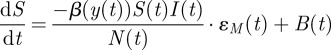
The differential equations describing the continuous time seasonal SIR model are

3.1

and

3.2

where S is the number of susceptibles, I is the number of infectives, N is the total population and β(t) is the time-varying transmission parameter. The function y(t) maps the overall horizon time with the elapsed time within the current year, making β(y(t)) a seasonal transmission parameter with periodicity of 1 year. Births into the population, B, and the population, N, are known time-varying system inputs, and the recovery rate (γ = 1/14 day) is a known scalar input. The variable ɛ_M represents multiplicative model noise, which is assumed to be log-normally distributed with a mean of 1. Additive noise was investigated, but, in those cases, the estimated values for the model noise showed an obvious temporal correlation with the data, indicating an unlikely model structure. However, the technique that we use can easily be modified to support different assumptions on the stochastic noise. Note that while this distribution can be an acceptable approximation for large datasets, where the number of cases never nears zero, for small datasets this distribution becomes invalid, as it does not allow for zero cases. In addition, as the reported number of cases must always be non-negative, the assumption of normally distributed measurement noise is only a reasonable approximation when the reported number of cases is not near zero. Given the size of the cities examined in this work and the number of reported cases over the given time horizons in the datasets, we find these assumptions acceptable here.

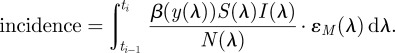
It is important to distinguish between incidence and prevalence in this problem formulation. The case count data are available for the incidence or the number of new cases reported over a given time interval. The model contains a state variable I(t) that is the prevalence of the disease, or the number of cases present at a given point in time. In a given reporting interval, integrating over the number of new cases gives the incidence,

3.3

To account for the difference in incidence and prevalence, a new state variable is introduced into the system through the following differential equation:

3.4

Here, Q(t) represents the cumulative incidence at time t and provides a state variable that can be used to evaluate the incidence over a particular interval.

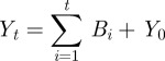
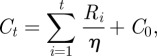
Not every individual that becomes infected is reported, which leads to case counts being under-reported. While there are various methods to estimate the reporting fraction η(t), in this work, we use a straightforward approach to estimate a linearly varying reporting fraction that is similar to the susceptible reconstruction approach described in Finkenstädt & Grenfell [8]. At the start of the estimation horizon, we assume that the number of cumulative cases, C₀, and cumulative births, Y₀, are unknown. Prior to widespread vaccination, almost every individual eventually contracted the disease. Therefore, on average, the cumulative number of new cases should equal the cumulative number of new births. For a constant reporting fraction, the cumulative cases and births are given by

3.5

and

3.6

where B_i is the reported number of births at time i, Y_t is the cumulative number of births at time t, R_i is the reported number of cases at time i and C_t is the cumulative number of cases at time t. We then minimize the sum-squared error between Y_t and C_t to estimate the reporting fraction η. For the case of our estimations with data from London and Bangkok, we extend this basic formulation to estimate a reporting fraction that varies linearly in time.

In our problem formulation, the estimated reporting fraction is treated as a known input for the estimation of the disease model parameters. To obtain a fit, the estimation formulation requires that we minimize some measure of the model and/or measurement noise subject to the infectious disease model described by the differential equations given in equations (3.1), (3.2) and (3.4).

There are two general approaches for the solution of large-scale dynamic parameter estimation problems similar to that considered here. The sequential approach considers only the degrees of freedom as optimization variables. This includes the initial conditions for I(t) and S(t), as well as a discretized time profile for the seasonal transmission parameter, β(t). A complete simulation of the forward problem is performed at each iteration of the optimization. To make use of modern gradient-based methods, derivative information must also be calculated along the entire time-series simulation. These derivatives can be expensive to calculate, especially for problems with many degrees of freedom. Furthermore, these derivatives can be noisy unless care is taken to ensure consistency of the integrator between runs [22]. Noise in the evaluation of sensitivities through the integrator can make these problems very challenging for the optimization solver. The simultaneous approach can be used to overcome these difficulties. In the simultaneous approach, all variables, including the states and the parameters, are discretized and treated as optimization variables. The entire discretized model is included as algebraic constraints in the optimization problem. The optimization problem resulting from the simultaneous approach can be larger than the sequential approach. However, this approach can be significantly faster than the sequential approach as the differential equation model is not converged at every iteration of the optimizer, but rather it is converged simultaneously as constraints to the optimization. Furthermore, accurate derivative information is easily obtained using modern automatic differentiation tools coupled with existing modelling frameworks. Recent advancements in nonlinear programming tools [23] allow efficient solution of sparse problems with hundreds of thousands of variables and constraints using standard desktop computing power [24–27]. In addition to potential efficiency gains, this simultaneous approach allows intuitive specification of additional constraints on the parameters and the state variables, including restrictions on the form of time-varying parameters. The flexibility of general nonlinear formulations coupled with the efficiency of large-scale algorithms make the simultaneous discretization approach coupled with general nonlinear programming tools an appropriate framework for efficient parameter estimation in nonlinear infectious disease models.

In this work, we use the simultaneous approach. We use collocation on finite elements to discretize the states into finite elements with fixed stepsize across the entire time horizon [28]. This converts the continuous differential equation model into an algebraic model that can be formulated as a nonlinear programming problem. A fifth-degree Gauss–Lobatto collocation technique is used to discretize the dynamics within these finite elements [29], and the discretized equations are included as equality constraints in the optimization problem. The effect of the instantaneous model noise, ɛ_M(t), on the system is approximated by introducing an unknown noise term between each of the finite elements.

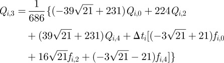
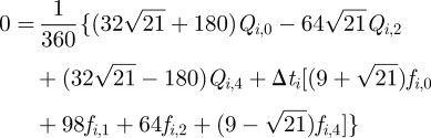
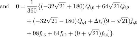
We illustrate this approach by showing the discretization of equation (3.4) within a single finite element i. Let t_i,j be the time associated with finite element i and collocation point j. With the fifth degree Gauss–Lobatto strategy, there are five collocation points for each finite element i (t_i,0 to t_i,4). The times t_i,0 to t_i,4 correspond to the locations of the collocation points within the finite element, where t_i,2 is the central collocation point located at the centre of the finite element. The time at t_i,1 is equal to , and the time at t₃ is equal to , where Δt_i is the length of finite element i. Letting Q_i,j be the value of and letting be the value of (equation (3.4)), the collocation equations become

3.7

3.8

3.9

3.10

In our formulation, we include model noise between these finite elements so that, while inside a finite element, equations (3.7)–(3.10) are exact and between finite elements there can be state discontinuities. With model noise between finite elements, there is little benefit in the use of a higher order method. However, we initialize our problem using the deterministic case where no model noise is present (model noise terms are fixed to zero), and, for this case, this discretization is a high-order method.

Our estimation formulation becomes,

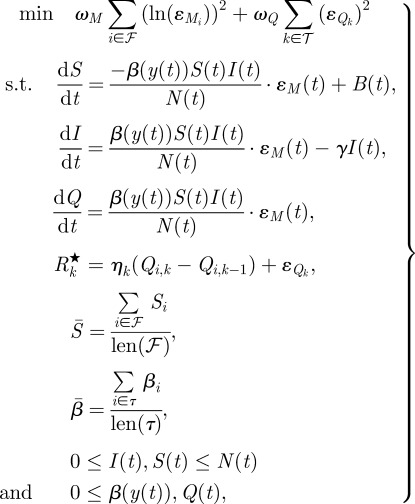3.11

where the differential equations are discretized using equations (3.7)–(3.10) and are shown here in their differential form for simplicity. The index k is a time point within the set of reporting times, 𝒯, while ℱ is the set of all finite elements used in the discretization. The reporting fraction η_k accounts for under-reporting over a given time interval spanning k − 1 to k, R_k^* is the actual reported incidence over a given time interval, is the measurement noise, and ω_M and ω_Q are weights for the noise terms. Based on the assumption of normality in and , the ratio of these weights should be equal to the inverse ratio of the variance in the estimated noise terms. Since the variances are not known a priori, a simple bisection approach is used to solve for the ratio of weights until 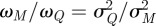, where is the calculated variance of the estimated noise terms , and is the calculated variance of the estimated noise terms (using standard mean squares). The estimation formulation is solved completely for each iteration of the bisection method. These weights determine the trade-off between model and measurement noise in the objective function. This straightforward approach was used since sensitivity studies (presented later in the paper) show that the estimates are relatively insensitive to the selection of these weights. However, other techniques have been proposed for determining these weights [3,30] and could also be used. Two additional variables are added to the problem formulation for use in calculating confidence regions. Here, is the average population of susceptibles over the time horizon and is the average value of β across the yearly set of discretizations τ.

It is important to point out that the objective function used in this formulation is the extended log-likelihood and only an approximation of the true log-likelihood for the parameters. The use of this likelihood for estimating parameters can cause considerable bias in both the parameters and their uncertainty [31]. In practice, bias may not always be observed, but care should be taken when evaluating results from this approach. The simulation study discussed in §4.1 shows no significant bias. However, if bias is a concern, then this efficient formulation and approach can still be used to initialize an unbiased approach.

This research focuses on the estimation of the seasonal transmission profile β(y(t)). While the case data show strong seasonality, the functional form of the transmission profile is unknown, so it is undesirable to force β to take the form of a particular periodic function (e.g. a sine function). Therefore, we discretize the transmission profile along finite-element boundaries, assuming a constant value through the finite element. In previous work, β(y(t)) was further restricted using total variation regularization [12]. However, in this work, it was found that regularization was unnecessary when the discretization of β matched the reporting interval of the case data. Some form of regularization or restriction of β would be necessary if β is discretized more finely than the reporting interval.

3.2. Estimation approach

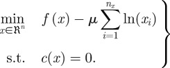
The nonlinear programming formulation described above was written in AMPL [32] and solved using Ipopt [33]. AMPL is an algebraic modelling language for optimization problems that provides first- and second-order derivatives using automatic differentiation. Ipopt is an open source primal–dual interior-point algorithm for solving nonlinear programming problems with inequality constraints, and is available through the COIN-OR foundation. This algorithm considers problems of the form,

3.12

where f(x) and c(x) are assumed to be twice differentiable, d^L and d^U are lower and upper bounds on a general function d, and x_L and x_U are lower and upper variable bounds on x. For ease of notation, the algorithm is described for the following problem formulation:

3.13

Note that general inequalities can be mapped to equality constraints and simple variable bounds through the addition of slack variables.

A significant challenge in the solution of these problems is identifying the active and inactive sets of variables (i.e. the set of variable bounds that are satisfied with equality at the solution versus the variables that are inside their bounds at the solution). With interior point methods, the inequality constraints are moved into the objective function using a log-barrier term to form the barrier subproblem,

3.14

This barrier subproblem is solved (approximately) for a sequence of barrier parameters. It can be shown, under mild conditions, that the sequence of solutions of the barrier subproblem converges to the solution of the original problem. From the first-order optimality conditions for (3.14), the following equations can be derived [33]:

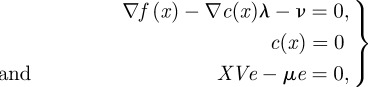3.15

where is the gradient of the objective function, is the transpose of the constraint Jacobian, λ and ν are the Lagrange multipliers for the equality constraints and inequalities, respectively, X is the diagonal matrix of x_i's, V is the diagonal matrix of ν_i's, and e is a vector of ones. A variant of Newton's method is used to solve equation (3.15) (with modifications to ensure that the directions are descent). Calculating the step requires the solution of the following linear system at each iteration:

3.16

where H is the Hessian of the Lagrange function and I is the identity matrix. This linear system is solved by first symmetrizing (3.16) and solving the so-called augmented system. Exact Hessian and Jacobian information is provided through AMPL. A filter-based line-search strategy is used to ensure global convergence. Further details concerning Ipopt can be found in the literature [33]. This approach has been used effectively on numerous large-scale nonlinear optimization problems [33–36].

4. Estimation results

To demonstrate the effectiveness of our approach, we first estimate parameters using simulated data from an SIR model. We then perform estimation using three real datasets from different settings. In our estimations, we use existing measles case count data for London [21], New York City [37,38] and Bangkok, which have been made available to us by the Thailand Ministry of Public Health [39]. These datasets also include yearly birth records and populations. The London dataset was chosen as it has been widely studied and provides a comparison of our model results with literature results. The New York City and Bangkok datasets are from cities with very different social settings and entirely different school holiday schedules. This allows us to compare estimated transmission profiles on locations with different school term schedules. The New York City data contain monthly reported case counts. The Bangkok data include monthly case counts and annual age distributions. There is regular active surveillance coupled to the passive surveillance in order to assess the performance of the passive surveillance system. The data are fully anonymized and laboratory confirmation is reported when available. The populations are assumed to vary linearly throughout the year, and the birth rates are assumed to be uniform throughout the year (figure 1).

Figure 1.

The reported number of cases for (a) London (1948–1964), (b) New York City (1944–1963) and (c) Bangkok (1975–1984).

To perform these estimations, we first format the data as required by the AMPL input data file format. We formulated the model shown in equation (3.11) with discretized differential equations using the algebraic modelling language AMPL [32]. Any modelling language coupled with a reliable large-scale nonlinear optimization solver could be used. We solve the problem using the open-source nonlinear solver Ipopt [33]. The weights for the objective function are found using the iterative process discussed previously. These weights are then fixed to find the confidence intervals and confidence regions.

Effective initialization is important for successful solution of general non-convex nonlinear programming problems. Here, all problems were initialized simply by setting all , , and and j collocation points, and . Here, ℱ is the set of finite elements and ℬ is the set of discretizations of β. While this is a very crude initialization, the formulation is robust, and we first solve the deterministic problem, fixing the model noise terms to zero, before solving the formulation with model noise terms included.

Our estimates showed a strong correlation between and , and the quality of our fit to the data differs dramatically outside of a narrow range of values. Confidence regions, derived from the likelihood-ratio test [40,41], are constructed as described by Rooney & Biegler [42] to show the region in which these values could be expected to lie. The regions are constructed over pairs of parameters by fixing the two parameters and reoptimizing over the remaining variables. In addition, likelihood ratios are used to construct confidence intervals for β by fixing each independently and allowing optimization over all other β_i's. These confidence regions and intervals were calculated using the extended likelihood, which is only an approximation of the true likelihood. The simulation study performed in §4.1 indicates that this approximation still provides reasonable confidence intervals. In the simulation study, the estimated confidence intervals are slightly more conservative than what the simulations would suggest as necessary.

4.1. Simulation

In order to test the estimation procedure using known parameter values, we perform stochastic simulations with an SIR model. The simulations were performed using Matlab. Our simulations used a constant population of 10 002 000, a recovery rate of 1/14 day, a birth rate of 2.95 per cent of the population per year and a reporting fraction of 1. To generate 20 years of case data, the deterministic model was integrated for 100 years to achieve a cyclic steady state. The final values from this simulation were used as the initial values for the stochastic simulation. The simulations were performed with the same model as that used for the estimation except that the time step used within the Matlab integration routine was a half day. Model noise was drawn from a log-normal distribution with mean 1 and σ = 0.05. Measurement noise was applied to the reported cases and was drawn from a normal distribution with mean 0 and an s.d. of 1000. While the assumption of normally distributed noise is not valid for datasets with a low number of reported cases, we assume it to be a reasonable distribution for our simulations since, in 10 000 simulations, the reported number of cases never fell below 2000.

The simulation was run 10 000 times with a reporting fraction of 1 to generate simulated case data, and estimations were run on each of these simulations using 12 finite elements per year. Figure 2 demonstrates that our estimation approach gives an extremely good estimate for β using data from the SIR simulations. The solid line shows the true parameter values used for all 10 000 simulations. The circles show the mean of the estimated values for the parameters as well as the 2.5 and 97.5 quantiles for the parameters estimated from all the simulations (giving the 95% confidence intervals for these estimates). The triangles show the estimated parameters from an estimation on a single randomly selected simulated dataset, and the dashed lines show the 95% confidence intervals generated for this estimation using the likelihood-ratio test. The true parameter values are included well inside these confidence intervals. The confidence intervals calculated from the likelihood-ratio test give more conservative intervals than what the 10 000 simulations would suggest are necessary and actually cover over 97 per cent of the values estimated from all 10 000 simulations. This is not unexpected given that the likelihood-ratio test confidence intervals are determined by fixing only one parameter at a time, allowing the other parameters to be optimized.

Figure 2.

The estimated transmission profile β (triangles) for a single dataset with 95% confidence intervals (dashed line) found using likelihoods. The true values of β used in the stochastic SIR simulation (solid line). The 2.5th, 50th and 97.5th quantiles of the estimates from the simulation (circles). (Online version in colour.)

Furthermore, the mean values of the estimated parameters over all 10 000 simulations agree with the true values used in the simulation. There is no significant bias observed in the estimate of the seasonal transmission parameters for the simulated data used in this study.

4.2. London

The time horizon studied for London was 1948–1964. The reporting fraction estimated using our approach varies linearly from 50.65 to 42.55 per cent over the time horizon studied. This dataset originally had case counts reported weekly; however, the dataset used here has combined the data so that case counts are given biweekly. These aggregated data were also used by Finkenstädt & Grenfell [8]. The estimation for London was performed using 26 finite elements per year, and the transmission profile was discretized so that each contained one finite element, giving 26 discretizations in β. The normalized estimated seasonal transmission profile for London is shown in figure 3. This figure also compares this result with the findings from Finkenstädt & Grenfell [8] and Cauchemez & Ferguson [11]. The time horizon used in this work and by Cauchemez & Ferguson [11] was the years 1948–1964, but the time horizon used by Finkenstädt & Grenfell [8] was the years 1944–1964. Despite the differing time horizons, it is clear that the seasonal pattern estimated from our approach is similar to these other results. The estimated profile appears to be correlated with school term holidays with the transmission profile decreasing during the school breaks that occur during the Easter holiday around biweek 8 and the summer holiday over biweeks 15–18. The Christmas holiday occurs at biweek 25, but there is no immediate effect captured in our estimates. The lack of any immediate effect could be owing to delays in reporting over the Christmas holidays [7].

Figure 3.

The transmission profile estimated for London by Finkenstädt & Grenfell [8] (dashed line), Cauchemez & Ferguson [11] (dotted line) and this work (solid line).

Figure 4 shows the non-normalized pattern for the estimated seasonal transmission profile. The estimated seasonal transmission parameter β(t) is on a per day basis, and the mean estimated value is . It does appear that our estimates may be shifted by one biweek relative to the school holidays, but this could be owing to a slight delay in reporting.

Figure 4.

The estimated transmission profile β with confidence intervals. School term holidays are shaded.

In figure 5a, we show nonlinear confidence regions for the mean transmission parameter value against the mean susceptible fraction over the mean population, , where the means were taken over the entire time horizon. As expected, this shows a dependence between the estimated values for and . The shape of these confidence regions provides some insight into why it may be difficult to accurately estimate the absolute magnitude of the transmission parameter. An increase in can be offset by a decrease in with little change in the objective function value. However, even though there is a difference in the absolute magnitude of the transmission parameter, we see little difference in the seasonal pattern estimated for the points within the indicated confidence region.

Figure 5.

A contour plot showing the contours of the left-hand side of the χ² test coming from the likelihood ratios (dashed lines) and the 95% confidence region (solid lines) for and divided by the population. Regions represent profile likelihood contours where likelihood ratios are calculated based on a re-optimization of all other parameters. The ‘plus symbol’ indicates the optimal estimated value. (a) London, (b) New York City and (c) Bangkok.

4.3. New York City

The estimation for New York City was performed using monthly reported data from 1944 to 1963. The reporting fraction estimated using our approach was almost constant around 11 per cent throughout the time horizon studied, and the reporting fraction was assumed constant in our estimates. The discretization strategy used 12 finite elements per year, and β is again assumed to be constant within each finite element. This gave 12 discretizations for the seasonal transmission profile β. The estimated seasonal transmission profile for New York City is shown in figure 6. This profile also shows strong correlation with the summer school term holidays that the New York City Board of Education reported occurring from mid-June to mid-September, or over the finite elements of approximately 6.5–9.5. There are school holidays around the end of the year; however, these holidays are much shorter than the reporting interval of the data.

Figure 6.

The estimated transmission profile β for New York City with shaded school term holidays.

Figure 5b shows the 95% confidence region for and . The optimal estimated was 11.1 per cent of the mean population, and the optimal estimated was 0.65. Our approach successfully estimates a seasonal transmission pattern that shows strong correlation to school terms.

4.4. Bangkok

In addition to data obtained from locations with a single large summer break, we also performed estimates using measles data for Bangkok, Thailand. Thailand has two school term holidays—one in the spring and one in the autumn. The estimation for Bangkok was performed using monthly reported case count data from the years 1975 to 1984. This dataset contains significant under-reporting with the estimated reporting fraction varying linearly from 1.1 per cent at the start of the time series to 4.5 per cent at the end of the time series. In addition, case counts are missing for the year 1979. The discretization strategy used 12 finite elements per year with β discretized by finite elements, giving 12 discretizations for β. As no data are available for the year 1979, these points were excluded in the objective function so that they would not affect the estimation while still allowing the model to simulate the states through this year. The estimated seasonal transmission profile β for Bangkok is shown in figure 7. This profile shows correlation with the two school term holidays that occur from the beginning of March until mid-May and the entirety of October, or over the finite elements of approximately 3–5 and 10–11. There is an obvious lag between our estimated drop in β and the start of the school holidays. This lag is probably owing to a lag in the reporting of case data. There are consistently extra cases reported in January resulting from a backlog of reports that are not processed at the end of the year owing to worker holidays. This suggests that cases are being reported as occurring when reports are processed rather than when the cases actually occurred, which would cause a lag in the estimates.

Figure 7.

The estimated transmission profile β for Bangkok with shaded school term holidays.

Figure 5c shows the 95% confidence region for and The optimal estimated was 5.5 per cent of the mean population, and the optimal estimated was 1.28.

4.5. Input sensitivity analysis

Our estimates are dependent upon the inputs we use in our model. We use recorded data for birth inputs and for population inputs, but no data are available for the reporting fraction and recovery rate, and we would like to know how sensitive our estimates are to the values used for these inputs. In addition, we use an iterative approach to set the weights in the objective function, and we would like to know how changing these weights will affect our estimates.

We first examined the effect of varying the reporting fraction on our estimates of β. To investigate this, we varied the value of the reporting fraction over a wide range about our estimated value. Using each new reporting fraction, we solved the same problem as before. Figure 8 shows the estimated average value of β for New York and the optimal objective function value as the reporting fraction changes. This plot shows that, even for small changes in the reporting fraction away from the estimated value, there is a significant decrease in the average value of β. The objective function values show that the best data fit occurs when the reporting fraction is where we also get the highest , and this reporting fraction is the same as that estimated using the approach described in §3.1.

Figure 8.

The estimated for New York City is shown as a function of the reporting fraction (solid line). The objective function value is also shown as a function of the reporting fraction (dotted line). (Online version in colour.)

In Bangkok, there is a significant difference in the reporting fraction at the beginning and at the end of the time horizon studied and a time-varying reporting fraction is needed. We use a linearly varying reporting fraction throughout the time horizon, and, for our sensitivity study, we keep the same slope as we estimated before. Figure 9 shows the estimated and optimal objective function values as the initial value of the reporting fraction is varied. Since the reporting fraction estimated previously is so low at the beginning of the time horizon and must be positive, we are unable to lower the initial value by more than about half of a per cent. Where we see the minimum in the optimal objective function value is also where we find the initial value of the reporting fraction that we estimated previously.

Figure 9.

The estimated for Bangkok is shown as a function of the initial value of the reporting fraction (solid line). The objective function value is also shown as a function of the reporting fraction (dotted line). (Online version in colour.)

The recovery rate can also affect the dynamics of the system, and different sources use different values (typically 1/13 or 1/14). Figure 10 shows the change in the estimated 's for New York City and Bangkok as the recovery rates are varied. For both cities, the changes in are not dramatic at any point, but simply change slowly throughout the range examined. This indicates that, for reasonable values for the recovery rate, our estimates are not dramatically affected.

Figure 10.

The values estimated for Bangkok (dotted line) and New York City (solid line) are shown as functions of the recovery rate. (Online version in colour.)

Finally, we also show the estimation results as a function of the ratio of the weights in the objective function. Here, we vary this ratio by two orders of magnitude on either side of the value found using our iterative procedure. Figure 11 shows the value of for both New York City and Bangkok as the weights are varied. The mean value of the transmission parameter changes little over a range of values near the estimated weights. Furthermore, the pattern exhibited by the estimated transmission parameter is nearly identical over this entire range.

Figure 11.

The values estimated for Bangkok (dotted line) and New York City (solid line) are shown as functions of the log of the ratio of the weights on the noise terms in the objective function. (Online version in colour.)

5. Discussion and conclusions

Successful estimation of parameters in dynamic models for childhood infectious diseases from time-series data presents several challenges. Typically, reported cases (the incidence) are the only available data, while there is little information about the susceptible population. Therefore, approaches must simultaneously estimate the prevalence and the unknown susceptible states. Furthermore, the case data are often significantly under-reported, the reporting interval is often longer than the serial interval of the disease and the models are highly nonlinear. This paper presented a nonlinear programming approach for estimating the unknown states and the seasonal transmission parameter using a continuous time model with both measurement and model noise.

Continuous time formulations offer several advantages over discrete time formulations for estimation of infectious disease models. Data can be handled in their native form regardless of the reporting interval. This was demonstrated by using biweekly reported data from London and monthly reported data from New York City and Bangkok. Using data in their native form is a significant advantage for diseases with short serial intervals, where it would be unreasonable to have data reported at the same interval.

The estimation approach outlined in this paper is highly efficient. The estimation formulation using continuous SIR models is a nonlinear optimization problem subject to differential equations as constraints. The use of the simultaneous or full-discretization approach produces a large-scale algebraic nonlinear programming problem. Nevertheless, efficient solutions are possible as the simulation is not converged at each iteration. The solution times for all estimations are shown in table 1. These are the full solution times, including the times required to initialize the problems and find the weights to be used in the objective functions. Significant reductions could be made by initializing the problem well and by giving good initial guesses for the objective function weights. Recent work by Hooker et al. [3] solves a similar problem formulation in approximately 2 h, the MCMC estimation performed by Cauchemez & Ferguson required approximately 20 h per run [11] and the plug-and-play method of He et al. [2] requires approximately 5 h. None of our estimations take longer than 5 min. The efficiency of this fully simultaneous approach opens the door to explore many more model structures efficiently and provides a framework that is scalable to large spatially distributed estimations.

Table 1.

Problem sizes and solution times of the London, New York City (NYC) and Bangkok (BKK) estimation problems studied in this paper.

	variables	constraints	CPU time (s)a
London	16 459	15 963	190
NYC	8929	8663	300
BKK	4477	4331	76

^aAll problems were solved on a 3 GHz Intel Xeon processor and times are reported is seconds.

Figure 5a–c shows a strong inverse correlation between the estimated and as seen by the narrow, elongated confidence regions. This result is not unexpected when compared with the approximate expression relating β to given by [20]. This relation gives a curve lying approximately through the middle of the 95% confidence region in figure 5a–c. These elongated regions indicate that the estimation is sensitive along this line and that care should be taken when interpreting absolute values for β or S. It should also be noted that the estimations produced nearly identical patterns in β(t) within these confidence regions.

More importantly, several recent publications have reported estimated values of the seasonal transmission parameter, and corresponding R₀ values, that are higher than estimates provided by Anderson & May [20]. For example, the reported estimates of He et al. [2] for London give R₀ = 57 with 95% confidence intervals of 37 and 60. There is significant complexity in finding R₀ values while considering seasonal transmission rates, and it is difficult to compare results arising from different model structures. Using the approximate relationship , we estimate R₀ = 13.3 in London with 95% confidence intervals of 12.1 and 14.3. Our estimates for New York City (R₀ = 9.1) and Bangkok (R₀ = 17.9) also give values for R₀ that appear consistent with values reported for measles by Anderson & May for other cities [20] and with values approximated using the average age of infection.

The estimated transmission profiles from all three cities show strong correlation with school holidays despite the very different holiday schedules seen between London, New York City and Bangkok. For Bangkok and New York City, there was a lag observed in the estimated transmission profiles that showed the drop in transmission as occurring after the holiday had begun. This is probably owing to a lag in reporting causing cases to be reported well after their occurrence and the incubation period of measles causing cases to be observed after the start of the holiday even though the infection occurred before the holiday.

This overall approach for estimating continuous time infectious disease models is reliable, flexible and efficient. Although the use of extended likelihood may not be guaranteed to provide unbiased estimates, the simulation results showed no evidence of bias. Solutions to the nonlinear programming problem were possible with a general initialization strategy, and effective parameter estimates are possible, even in the face of challenging sets of data that contain missing years, severe under-reporting and significant noise. It is straightforward to switch between diseases with different serial intervals or datasets with different reporting intervals. The approach is independent of model specifics. For example, it would be straightforward to add additional compartments to the model, such as adding an E compartment to make an SEIR model that would account for individuals that have been exposed to a disease but cannot yet infect susceptibles. One could also add a compartment to account for portions of the population that were vaccinated against a disease. Furthermore, the approach is highly efficient, making it appropriate for much larger problem formulations, or for rapid exploration and comparison of multiple model structures. Using this flexible framework, we propose to address two important advances in future work. First, standard assumptions with the SIR model give exponential distributions in age dependence of cases. This is contrary to the age-distributed case data we have for these locations. We propose to develop an age- and time-discretized model to estimate seasonal age-dependent transmission parameters using this approach.

Also, while this work focused on estimating transmission parameters for individual large cities, another interesting problem for health officials is looking at a spatial model of disease spread. For accurate estimation of disease dynamics in small cities where fade-out is observed, information is needed regarding the transmission of the disease from a large city where the disease is endemic to the small city. The approach described in this paper is appropriate for the estimation of large-scale, spatially distributed, nonlinear differential equation models and will be a subject of future research.

References

- 1.Bobashev G. V., Ellner S. P., Nychka D. W., Grenfell B. T. 2008. Reconstructing susceptible and recruitment dynamics from measles epidemic data. Math. Popul. Stud. 8, 1–29 10.1080/08898480009525471 (doi:10.1080/08898480009525471) [DOI] [Google Scholar]
- 2.He D., Ionides E. L., King A. A. 2010. Plug-and-play inference for disease dynamics: measles in large and small populations as a case study. J. R. Soc. Interface 7, 271–283 10.1098/rsif.2009.0151 (doi:10.1098/rsif.2009.0151) [DOI] [PMC free article] [PubMed] [Google Scholar]
- 3.Hooker G., Ellner S. P., Roditi L. D. V., Earn D. J. D. 2011. Parameterizing state-space models for infectious disease dynamics by generalized profiling: measles in Ontario. J. R. Soc. Interface 8, 961–974 10.1098/rsif.2010.0412 (doi:10.1098/rsif.2010.0412) [DOI] [PMC free article] [PubMed] [Google Scholar]
- 4.Ferguson N. M., Cummings D. A. T., Cauchemez S., Fraser C., Riley S., Meeyai A., Iamsirithaworn S., Burke D. S. 2005. Strategies for containing an emerging influenza pandemic in southeast asia. Nature 437, 209–214 10.1038/nature04017 (doi:10.1038/nature04017) [DOI] [PubMed] [Google Scholar]
- 5.Hethcote H. W. 2000. The mathematics of infectious diseases. SIAM Rev. 42, 599–653 10.1137/S0036144500371907 (doi:10.1137/S0036144500371907) [DOI] [Google Scholar]
- 6.Soper H. E. 1929. The interpretation of periodicity in disease prevalence. J. R. Stat. Soc. 92, 34–73 10.2307/2341437 (doi:10.2307/2341437) [DOI] [Google Scholar]
- 7.Fine P. E., Clarkson J. A. 1982. Measles in England and Wales I: an analysis of factors underlying seasonal patterns. Int. J. Epidemiol. 11, 5–14 10.1093/ije/11.1.5 (doi:10.1093/ije/11.1.5) [DOI] [PubMed] [Google Scholar]
- 8.Finkenstädt B. F., Grenfell B. T. 2000. Time series modelling of childhood diseases: a dynamical systems approach. J. R. Stat. Soc. C 49, 187–205 10.1111/1467-9876.00187 (doi:10.1111/1467-9876.00187) [DOI] [Google Scholar]
- 9.Xia Y., Bjornstad O. N., Grenfell B. T. 2004. Measles metapopulation dynamics: a gravity model for epidemiological coupling and dynamics. Am. Nat. 164, 267–281 10.1086/422341 (doi:10.1086/422341) [DOI] [PubMed] [Google Scholar]
- 10.Glass K., Xia Y., Grenfell B. 2003. Interpreting time-series analyses for continuous-time biological models–measles as a case study. J. Theor. Biol. 223, 19–25 10.1016/S0022-5193(03)00031-6 (doi:10.1016/S0022-5193(03)00031-6) [DOI] [PubMed] [Google Scholar]
- 11.Cauchemez S., Ferguson N. M. 2008. Likelihood-based estimation of continuous-time epidemic models from time-series data: application to measles transmission in London. J. R. Soc. Interface 5, 885–897 10.1098/rsif.2007.1292 (doi:10.1098/rsif.2007.1292) [DOI] [PMC free article] [PubMed] [Google Scholar]
- 12.Word D. P., Abbott G. H., III, Cummings D. A. T., Laird C. D. 2010. Estimating seasonal drivers in childhood infectious diseases with continuous time and discrete-time models. In Proc. of ACC 2010, Baltimore, MD, 30 June–2 July 2010, pp. 5137–5142 [Google Scholar]
- 13.Greenhalgh D., Moneim I. A. 2003. SIRS epidemic model and simulations using different types of seasonal contact rate. Syst. Anal. Modell. Sim. 43, 573–600 10.1080/023929021000008813 (doi:10.1080/023929021000008813) [DOI] [Google Scholar]
- 14.Schenzle D. 1984. An age-structured model of pre and post-vaccination measles transmission. Math. Med. Biol. 1, 169–191 10.1093/imammb/1.2.169 (doi:10.1093/imammb/1.2.169) [DOI] [PubMed] [Google Scholar]
- 15.Cintrón-Arias A., Banks H., Capaldi A., Lloyd A. L. 2009. A sensitivity matrix based methodology for inverse problem formulation. J. Inverse Ill-posed Problems 15, 545–564 10.1515/JIIP.2009.034 (doi:10.1515/JIIP.2009.034) [DOI] [Google Scholar]
- 16.Keeling M. J. 1997. Modelling the persistence of measles. Trends Microbiol. 5, 513–518 10.1016/S0966-842X(97)01147-5 (doi:10.1016/S0966-842X(97)01147-5) [DOI] [PubMed] [Google Scholar]
- 17.Bartlett M. S. 1957. Measles periodicity and community size. J. R. Stat. Soc. A (General) 120, 48–70 10.2307/2342553 (doi:10.2307/2342553) [DOI] [Google Scholar]
- 18.Finkenstädt B. F., Bjornstad O. N., Grenfell B. T. 2002. A stochastic model for extinction and recurrence of epidemics: estimation and inference for measles outbreaks. Biostatistics 3, 493–510 10.1093/biostatistics/3.4.493 (doi:10.1093/biostatistics/3.4.493) [DOI] [PubMed] [Google Scholar]
- 19.Ramsay J. O., Hooker G., Campbell D., Cao J. 2007. Parameter estimation for differential equations: a generalized smoothing approach. J. R. Stat. Soc. B (Stat. Methodol.) 69, 741–796 10.1111/j.1467-9868.2007.00610.x (doi:10.1111/j.1467-9868.2007.00610.x) [DOI] [Google Scholar]
- 20.Anderson R. M., May R. M. 1991. Infectious diseases of humans: dynamics and control. New York, NY: Oxford University Press Inc [Google Scholar]
- 21.Bjornstad O. N., Finkenstädt B., Grenfell B. T. 2002. Dynamics of measles epidemics: estimating scaling of transmission rates using a time series SIR model. Ecol. Monogr. 72, 169–184 10.1890/0012-9615(2002)072[0169:DOMEES]2.0.CO;2 (doi:10.1890/0012-9615(2002)072[0169:DOMEES]2.0.CO;2) [DOI] [Google Scholar]
- 22.Betts J. T., Kolmanovsky I. 2002. Practical methods for optimal control using nonlinear programming. Appl. Mech. Rev. 55, B68. 10.1115/1.1483351 (doi:10.1115/1.1483351) [DOI] [Google Scholar]
- 23.Gould N. I. M., Orban D., Toint P. 2004 Numerical methods for large-scale nonlinear optimization. RAL-TR-2004-032, Central Laboratory of the Research Councils, UK. [Google Scholar]
- 24.Zavala V. M., Biegler L. T. 2006. Large-scale parameter estimation in low-density polyethylene tubular reactors. Ind. Eng. Chem. Res. 45, 7867–7881 10.1021/ie060338n (doi:10.1021/ie060338n) [DOI] [Google Scholar]
- 25.Zavala V. M., Laird C. D., Biegler L. T. 2008. Interior-point decomposition approaches for parallel solution of large-scale nonlinear parameter estimation problems. Chem. Eng. Sci. 63, 4834–4845 10.1016/j.ces.2007.05.022 (doi:10.1016/j.ces.2007.05.022) [DOI] [Google Scholar]
- 26.Laird C. D., Biegler L. T., van Bloemen Waanders B. G., Bartlett R. A. 2005. Contamination source determination for water networks. ASCE J. Water Resour. Plann. Manage. 131, 125. 10.1061/(ASCE)0733-9496(2005)131:2(125) (doi:10.1061/(ASCE)0733-9496(2005)131:2(125)) [DOI] [Google Scholar]
- 27.van Bloemen Waanders B. G., Bartlett R. A., Biegler L. T., Laird C. D. 2003. Nonlinear programming strategies for source detection of municipal water networks. In Proc. World Water & Environmental Resources Congress 2003 and Related Symposia, Philadelphia, PA, 23–26 June 2003 (eds P. Bizier & P. DeBarry), p. 38. Reston, VA: ASCE [Google Scholar]
- 28.Zavala V. M. 2008 Computational strategies for the optimal operation of large-scale chemical processes. PhD Thesis, Carnegie Mellon University, PA, USA. [Google Scholar]
- 29.Herman A. L., Conway B. A. 1996. Direct optimization using collocation based on high-order Gauss–Lobatto quadrature rules. J. Guid. Control Dynam. 19, 592–599 10.2514/3.21662 (doi:10.2514/3.21662) [DOI] [Google Scholar]
- 30.Varziri M. S., Poyton A. A., McAuley K. B., McLellan P. J., Ramsay J. O. 2008. Selecting optimal weighting factors in iPDA for parameter estimation in continuous-time dynamic models. Comput. Chem. Eng. 32, 3011–3022 10.1016/j.compchemeng.2008.04.005 (doi:10.1016/j.compchemeng.2008.04.005) [DOI] [Google Scholar]
- 31.Lee Y., Nelder J. A., Pawitan Y. 2006. Generalized linear models with random effects: unified analysis via H-likelihood. Boca Raton, FL: CRC Press [Google Scholar]
- 32.Fourer R., Gay D. M., Kernighan B. W. 1993. AMPL: a modeling language for mathematical programming. Danvers, MA: The Scientific Press [Google Scholar]
- 33.Wächter A., Biegler L. T. 2006. On the implementation of an interior-point filter line-search algorithm for large-scale nonlinear programming. Math. Programm. 106, 25–57 10.1007/s10107-004-0559-y (doi:10.1007/s10107-004-0559-y) [DOI] [Google Scholar]
- 34.Zhu Y., Legg S., Laird C. D. 2010. Optimal design of cryogenic air separation columns under uncertainty. Comput. Chem. Eng. 34, 1377–1384 [Google Scholar]
- 35.Zhu Y., Legg S., Laird C. D. 2010. A multiperiod nonlinear programming approach for operation of air separation plants with variable power pricing. AIChE J. 57, 2421–2430 10.1002/aic.12464 (doi:10.1002/aic.12464) [DOI] [Google Scholar]
- 36.Zhu Y., Legg S., Laird C. D. 2011. Optimal operation of cryogenic air separation systems with demand uncertainty and contractual obligations. Chem. Eng. Sci. 66, 953–963 10.1016/j.ces.2010.11.039 (doi:10.1016/j.ces.2010.11.039) [DOI] [Google Scholar]
- 37.Yorke J. A., London W. P. 1973. Recurrent outbreaks of measles, chicken pox, and mumps. Am. J. Epidemiol. 98, 469–482 [DOI] [PubMed] [Google Scholar]
- 40.Seber G., Wild C. 1989. Nonlinear regression. New York, NY: Wiley [Google Scholar]
- 41.Gallant A. R. 1987. Nonlinear statistical models. New York, NY: Wiley [Google Scholar]
- 42.Rooney W. C., Biegler L. T. 2004. Design for model parameter uncertainty using nonlinear confidence regions. AIChE J. 47, 1794–1804 10.1002/aic.690470811 (doi:10.1002/aic.690470811) [DOI] [Google Scholar]
- 38.The City of New York Department of Health. 1964. Vital statistics 1956 to 1963. New York, NY: Bureau of Records and Statistics, USA. [Google Scholar]
- 39.Bureau of Epidemiology. 1983 Annual epidemiological surveillance report: measles. Bangkok, Thailand: Department of Disease Control, Ministry of Public Health, Thailand. [Google Scholar]