The nanometre-scale physiology of bone: steric modelling and scanning transmission electron microscopy of collagen–mineral structure

Abstract

The nanometre-scale structure of collagen and bioapatite within bone establishes bone's physical properties, including strength and toughness. However, the nanostructural organization within bone is not well known and is debated. Widely accepted models hypothesize that apatite mineral (‘bioapatite’) is present predominantly inside collagen fibrils: in ‘gap channels’ between abutting collagen molecules, and in ‘intermolecular spaces’ between adjacent collagen molecules. However, recent studies report evidence of substantial extrafibrillar bioapatite, challenging this hypothesis. We studied the nanostructure of bioapatite and collagen in mouse bones by scanning transmission electron microscopy (STEM) using electron energy loss spectroscopy and high-angle annular dark-field imaging. Additionally, we developed a steric model to estimate the packing density of bioapatite within gap channels. Our steric model and STEM results constrain the fraction of total bioapatite in bone that is distributed within fibrils at less than or equal to 0.42 inside gap channels and less than or equal to 0.28 inside intermolecular overlap regions. Therefore, a significant fraction of bone's bioapatite (greater than or equal to 0.3) must be external to the fibrils. Furthermore, we observe extrafibrillar bioapatite between non-mineralized collagen fibrils, suggesting that initial bioapatite nucleation and growth are not confined to the gap channels as hypothesized in some models. These results have important implications for the mechanics of partially mineralized and developing tissues.

1. Introduction

While bone's hierarchical structure has been elucidated at the millimetre and micrometre scales, its nanostructure is poorly understood. Bulk material characterization shows bone to be a composite with approximately 40 vol% type I collagen and approximately 50 vol% of a stiff, carbonated apatite mineral (‘bioapatite’; the remaining approx. 10 vol% consists of water and non-collagenous proteins) [1]. Defects in any of these components can result in significant pathology, e.g. osteogenesis imperfecta [2]. Understanding bone's nanostructure may allow us to better evaluate and interpret bone pathologies and to develop biomimetic strategies for tissue engineering of bone and of partially mineralized tissues.

Studies of developing bone and of bone with defects in collagen indicate that a collagen template is first created before the nucleation of bioapatite crystals (for reviews, see [1,3]). In the widely accepted Hodge–Petruska [4] model for the steric arrangement (packing) of collagen molecules in the bone (figure 1a,b), triple-helix type I collagen molecules (300 nm in length, 1.5 nm in diameter, assumed to be straight and rod-like) pack together to form microfibrils (for a glossary of terms, see electronic supplementary materials). Microfibrils can be defined as an assemblage of five strands of stacked collagen molecules. Within each strand, the collagen is stacked with an approximately 36 nm gap space between the N-terminus of one collagen molecule and the C-terminus of the succeeding molecule. The five strands are staggered (along their stacking direction) with respect to each other by approximately 67 nm (approx. one-fourth the length of a collagen molecule, hence termed quarter-staggered). Alternatively, microfibrils can be defined as an assemblage of five individual collagen molecules arranged in parallel and quarter-staggered along their axial direction (see §2.5). These definitions differ in the manner in which the microfibrils pack (in two or three dimensions, respectively) to form larger structures (up to 0.5 µm diameter) termed fibrils.

Figure 1.

(a) The model for packing of collagen molecules in bone, as first presented by Hodge & Petruska [4]. Collagen molecules, assumed straight and rod-like, are stacked end-to-end with approximately 36 nm of space or ‘gap’ between them (note that the molecule diameters are disproportionately large for illustration purposes). The stacking of adjacent molecules within a microfibril is quarter-staggered (see text). Four of the five quarter-staggered arrangements per microfibril are shown and indicated by Arabic numerals. In the plane normal to the quarter-staggered molecules, collagen molecules are arranged in parallel planar arrays (indicated by Greek letters). Bioapatite crystals are postulated to nucleate and grow within the gap spaces between N- and C-termini of collagen molecules in fibrils. (b) In this model, it was proposed that bioapatite grows into the intermolecular spaces within a fibril in the later stages of mineralization [4,5]. (c) An updated model based on synchrotron studies described a right-hand helical twist along the length of the collagen molecules [6,7]. Fibrils formed from microfibrils assembled in this manner likely have insufficient intermolecular spaces large enough to accommodate bioapatite nanocrystallites outside of the gap spaces. (d) Gap spaces accommodate bioapatite platelets. The collagen molecules in (c) and (d) are shown with tapered ends to better show their relative positions in three dimensions. Note that for (c) and (d), microfibrils are three dimensional bundles of collagen molecules, unlike the planar arrays shown in (a) and (b).

This picture has been modified recently by the synchrotron studies of Orgel et al. [6,7], which demonstrated that collagen molecules are not rod-like but are right-hand helically twisted in a discontinuous manner along the length of the microfibrils and are bound together at specific locations (figure 1c). The N-terminus of each collagen molecule is bound to two (one inter- and one intra-microfibrillarly) abutting collagen molecules. Neighbouring microfibrils interdigitate, imposing order upon a mildly twisted lattice that forms fibrils. Microfibril interdigitation may explain the previously inferred presence of continuous, gap channels in the fibril structure, formed by the hypothesized alignment of gap spaces in the neighbouring microfibrils [8]. Interdigitation may also explain why individual microfibrils have not been isolated from fibrils [7]. In the next level of structural hierarchy, fibrils close-pack into larger lamellar structures to form tissue fibres (3–7 μm in diameter).

Bioapatite crystals nucleate and grow within this hierarchal collagen structure to form bone. Based on detailed transmission electron microscopy (TEM) studies, Hodge and Petruska identified periodically staggered gaps between N- and C-termini of collagen molecules in fibrils and argued that a significant mass of bioapatite can reside in those gap channels without significant distortion of the fibril structure [4,9,10]. They further concluded that bioapatite grows in these channels during early mineralization. However, it was soon realized that the gap channels did not have sufficient volume to contain all of the bioapatite in fully calcified bone. Therefore, Katz & Li [11] proposed that, in the later stages of mineralization, bioapatite must grow out of gap channels into the ‘intermolecular spaces’ that are between adjacent collagen molecules but within collagen fibrils (figure 1b), likely distorting the fibrillar structure. Nucleation of bioapatite within the intermolecular space has also been proposed recently [12]. The conjecture that bioapatite nucleation and growth occur within collagen fibrils has been supported by a number of TEM [8,13–16] as well as neutron and X-ray diffraction (XRD) [17–19] studies of bone and calcified tendon. Furthermore, estimates of the gap space and intermolecular volume within a fibril indicated that together they could accommodate most (approx. 75%) of the bioapatite in bone [11], and that was generally considered an underestimation of the available volume [1].

The Hodge–Petruska model was limited by its representation of collagen packing in three dimensions, with parallel packing of straight rod-like collagen molecules providing continuous and straight intermolecular volumes for bioapatite platelets to occupy (cf. figure 1b and illustrations in Olszta et al. [12]). On the contrary, the recent detailed description by Orgel et al. [6,7], of microfibrils assembled from helically twisted collagen molecules, which interdigitate with adjacent microfibrils, is that of a more geometrically constrained intermolecular space with no obvious capacity to accommodate nanometre-sized platelets of bioapatite outside of the gap channels.

Other results from the last two decades further challenged the established model for bone's nanostructure. Bonar et al. [20], using neutron diffraction data from fully mineralized mature bovine bone, calculated that the gap channels and overlap regions within fibrils could together accommodate only approximately 25 per cent of the bioapatite in bone. However, the result received little attention, possibly because it conflicted with previous estimates, as well as with inferences drawn from TEM [5,8,13–16] and from neutron and XRD studies [17–19,21,22]. In contrast to those studies, high-voltage TEM tomography [23,24], analytical TEM [25], conventional TEM [26,27] and atomic force microscopy (AFM) [27–29] studies report evidence for extrafibrillar in addition to intrafibrillar bioapatite. Estimates of the volume fraction of extrafibrillar space in bone of up to approximately 60 per cent suggest that a significant mass of bioapatite could be accommodated external to the fibrils [24]. Furthermore, models of nanocomposite materials based on measured elastic properties of canine bone and narwhal dentin predict at least 50 per cent of the bone bioapatite is external to the fibrils [30].

How bioapatite is distributed in bone as a function of anatomical location, maturity, remodelling state and species has not been fully characterized. There could be significant dissimilarity between different types of bone which might explain the different conclusions drawn from the previously mentioned studies. To further test the hypothesis that bioapatie resides predominantly within collagen fibrils of mature bone in a mammal, we performed high-resolution quantitative scanning (S)-TEM nanocharacterizations using electron energy loss spectroscopy (EELS) imaging and high-angle annular dark-field (HAADF) imaging to measure the spatial distribution of bioapatite and collagen within mouse bone. We also developed a steric model of bone's structure to predict the concentration of bioapatite in fibrils. Our scanning transmission electron microscopy (STEM)–EELS elemental maps directly image fibrillar gap channels formed by the alignment of gap spaces in adjacent microfibrils and demonstrate that most of the intrafibrillar bioapatite is present in these gap channels [31]. Although TEM-measured bioapatite concentrations in bone are difficult to interpret because of challenges with TEM specimen preparation, our STEM–EELS measurements suggest that gap channels contain at least a factor of 1.5 more bioapatite than what is present in the intermolecular space of the fibrils. Our steric model predicts that the gap channels can accommodate as high as 42 per cent of the total bioapatite in bone (i.e. 21 vol.% out of the total 50 vol.% bioapatite in bone). Therefore, our steric model together with our STEM–EELS measurements place an upper bound on the amount of bioapatite than be accommodated within fibrils at 70 per cent of the total bioapatite in bone (i.e. 35 vol.% out of the total 50 vol.%). Therefore, additional bioapatite must be present external to the fibrils in the mouse bones we studied, as confirmed by our STEM imaging.

2. Material and methods

2.1. Transmission electron microscopy specimen preparation

The humeral head with the supraspinatus tendon attached was dissected from 56-day-old CD-1 mice. Five mice were prepared for analysis (yielding one sample each) and usable data were acquired from three of those samples. Specimens were cut in the coronal plane with a scalpel blade to expose the endosteal cortical surface of the humeral head. Specimens for TEM examination were fixed in a solution of 4 per cent paraformaldehyde and 2.5 per cent gluteraldehyde in 0.1 M cacodylate buffer overnight. A secondary (post) fixation was performed in a solution of 1 per cent osmium tetroxide in 0.1 M cacodylate buffer (pH 7.2–7.4) for 1 h to prevent extraction of some lipids during ethanol dehydration. The specimens were processed through a gradual ethanol dehydration sequence: 50 per cent ethanol for 10 min, 70 per cent for 30 min, 95 per cent for 45 min (two times), and 100 per cent for 1 h (three times). The specimens were then washed in propylene oxide for 15 min (two times). Increasing concentrations of Eponate 12 resin mixed in propylene oxide (1 : 1 overnight under vacuum or with agitation, then 1 : 0 for 4–6 h with agitation) were infiltrated into the specimens. A final infiltration of fresh Eponate 12 was performed for 1 h prior to polymerization overnight at 65°C. A Leica EM UC6 ultramicrotome was used to prepare approximately 70 nm thick TEM thin sections, which were mounted on amorphous-carbon (a-C)-coated Cu TEM grids. Two to three sections per sample were analysed. A total of 33 STEM–EELS runs were performed (each one taking approx. 12 h to complete); 14 of these runs produced data free of contamination and artefact and were included in this study.

2.2. Transmission electron microscopy nanocharacterization: instrument

The nanostructure of the specimens was characterized using a JEOL JEM-2100F field emission scanning transmission electron microscope equipped with high-resolution pole piece and a Schottky field emission gun: 0.5 nA at 1 nm full width at half-maximum (FWHM) probe diameter. This instrument was operated at 200 kV and at that energy has a rated point resolution of 0.23 nm and a lattice resolution of 0.1 nm. The instrument is equipped with a Gatan Model 863 Tridiem electron energy-imaging filter (GIF) with spectrum imaging package (STEMPack) capable of EELS, EELS spectral imaging, and electron energy-filtered (EF) imaging. The GIF is instrumented with an Ultrascan 1000 2048 × 2048 pixel, 16-bit, fibre optically coupled, peltier-cooled, charged-coupled device (CCD) camera. For STEM imaging, the instrument is equipped with Gatan Model 805 dark-field (DF) and bright-field (BF) STEM detectors as well as a Gatan Model 806 HAADF STEM detector capable of z-contrast imaging. For conventional TEM imaging, the instrument has a retractable Gatan Orius SC1000B 2672 × 4008 pixels, 14 bit, fibre optically coupled, peltier-cooled, CCD camera mounted on-axis directly above the GIF.

2.3. Transmission electron microscopy nanocharacterization: methods

Shortly after insertion into the TEM instrument column, the specimen was subjected to a greater than 1 h beam shower to fix any hydrocarbons (and prevent spot contamination) prior to exposing the specimen to a focused approximately 1 nm FWHM diameter probe. Regions of the specimen that overhung holes in the a-C support film that coated the TEM grids were examined to avoid C edge signal from the support film. The position of the Gatan HAADF detector with respect to the GIF along the electron optical axis of the microscope allowed simultaneous acquisition of STEM–HAADF images along with STEM–EELS spectral images.

Specimens were imaged in STEM mode using the HAADF detector, which can measure electrons at high scattering angles (in our case, the range 36.8 ± 0.1 to 128.0 ± 0.4 mrad) where scattering is approximately incoherent. Specimens were also imaged using the GIF to produce elemental maps from STEM–EELS spectral images. The following conditions were used during collection of STEM–EELS spectral images: a collection angle of 2β = 22.66 ± 0.06 mrad, a 5 mm diameter spectrometer entrance aperture, and an energy dispersion of 0.2 eV channel⁻¹. Spectra were collected over a 409.6 eV range starting at approximately 232 eV (see electronic supplementary material, figure S1). Spectra were corrected for dark current and channel-to-channel gain variation of the GIF CCD detector array and collected in the diffraction mode of the TEM (i.e. image coupling to the EELS spectrometer). The acquisition of an EELS spectral image consisted of collecting a core-loss spectrum at each pixel within a STEM region of interest (ROI). The dimensions of the ROI were approximately 60 × 200 pixels and spectrum acquisition times were 2–4 s per pixel (up to 12 h were required to collect an EELS spectral image). Any dataset that exhibited evidence of hydrocarbon contamination by the probe during the EELS spectrum image acquisition was discarded. The spectra (see electronic supplementary material, figure S1) were processed using Gatan Digital Micrograph by fitting a power-law background to each of the pre-edge regions. Proper background subtraction is critical (and sometimes non-trivial) in the analysis of spectral images. Summed spectra from 2 × 2 pixel regions across each map were examined to determine the quality of the background fits. If the fitted background appeared inappropriate (i.e. deviated significantly from the expected background) for any of the core-loss edges somewhere in a spectral image, the fitting parameters were iteratively modified. No systematic deviations were observed in any of our spectral images, i.e. no deviations were found to consistently be present at the periodically spaced gap channels or intermolecular spaces. While it is difficult to find fitting parameters that remove all deviations entirely, any deviations that remained were random with respect to the pixel location and their effects should average out in column average plots. The background was subtracted from the edge signal, which was then integrated over a wide window. The integration windows were all set to 45 eV so that effects of thickness variations in the specimen (i.e. plural scattering effects) would be the same for each of the measured elements (with the exception of the N-K edge, which was set to 40 eV to avoid integrating over the Ca-L₁ edge signal). Ratios of integrated EELS core-loss signal between two elements were converted to their corresponding atomic ratios using partial cross sections that were calculated from theoretical Hartree–Slater models. Unlike maps of EELS core-loss signal, maps of relative elemental compositions are not influenced by variations in specimen thickness and electron diffraction [32]. Further discussion of EELS spectra map analysis can be found in the electronic supplementary material.

2.4. Interpretation of scanning transmission electron microscopy–high-angle annular dark-field and electron energy loss spectroscopy images

Bioapatite is a carbonated and compositionally complex form of the mineral hydroxylapatite (Ca₅(PO₄)₃(OH)), whose structure permits chemical substitution of various secondary elements and, thus, variation in composition [1,33–38]. Collagen fibrils are primarily made up of the amino acids glycine-NH₂CH₂COOH, proline-C₅H₉NO₂ and hydroxyproline-C₅H₉O₃N with trace levels of other elements present. In bone tissue, nearly all of the Ca is contained within the bioapatite. While both bioapatite and collagen fibrils contain C (bioapatite contains up to six or more wt.% carbonate (CO₃²⁻)) [1], the majority of the C is contained in the collagen molecules. In EELS elemental maps, Ca and C can, therefore, be used as tracers for bioapatite and collagen, respectively.

In STEM–HAADF imaging, the high-angle scattering cross section for the volume probed by the electron beam is approximately proportional to the square of the mean atomic number in that volume. Therefore, scattering from heavy atoms will be more intense than from light atoms, producing an image with atomic z-contrast. In other words, the image intensity (for specimens of uniform thickness) is approximately proportional to the square of the mean atomic number.

2.5. Nanometre-scale steric model of bone

We developed a steric model for collagen fibrils consisting of collagen molecules and bioapatite platelets using computer-aided design software (SolidWorks, Concord, MA, USA; figures 2 and 3, see also animations in electronic supplementary material). Collagen molecules were approximated by 1.5 nm diameter, 300 nm length cylinders (figure 2a).

Figure 2.

Steric model of bioapatite platelet accumulation within collagen fibrils. (a) Bioapatite is shown in red, and collagen molecules are shown in grey (note that spatial scales do not match). (b) The basic unit used to construct the steric model (which can be viewed as a definition of a microfibril) consisted of five individual collagen molecules in a quarter-staggered arrangement labelled 0, 1/4, 1/2, 3/4 and 1 to indicate their relative height with respect to a horizontal plane. Collagen molecules were helically coiled along their length with a coil pitch of 3 μm. (c) These units were three-dimensionally stacked and packed (as described in the text) to form fibrils. (d) An edge-on view of bioapatite platelets inserted in one set of gaps between abutting collagen molecules is shown. (e) Four possible orientations of bioapatite platelets are shown in successive gap channels in the fibril. The three-dimensional steric model can also be visualized in the video that is available as electronic supplementary material. For visual clarity, the collagen molecules are drawn as straight rods rather than helically twisted molecules in all panels except (b).

Figure 3.

(a) Steric model and schematic cross sections at the gap channels. In the cross-sectional views, grey circles represent collagen molecules in the gap channel and green circles represent the projected location of collagen molecules that are present in the overlap space, but are not present in the gap channel. For any given gap channel, there are five possible orientations in which bioapatite crystals can be virtually inserted. For illustration purposes, these five insertion orientations are drawn in successive gap channels in a fibril. This is not necessarily the periodic pattern of these orientations in bone; the pattern (if periodic) or distribution of orientations (if the pattern is random) of bioapatite platelets in bone is unknown. These orientations for bioapatite insertion have packing densities of bioapatite with relative concentrations of approximately 25 : 12 : 9 for the orientations no.3 and no.4 : no.2 and no.5 : no.1. Orientations 3 and 4 represent the highest possible packing of bioapatite platelets and provide an upper limit of approximately 21 vol.% for bioapatite in gap channels of bone. (b) An elemental map of collagen fibrils in a mineralized region of bone that suffered break up and fracture by the diamond knife. The images on the top show carbon-rich regions (i.e. collagen) in green and calcium-rich regions (i.e. bioapatite) in red. A three-dimensional structural model of a mineralized fibril is shown in the middle bottom position of the panel. Note that bioapatite (i.e. Ca) occurs abundantly throughout the tissue and is also concentrated in the intrafibrillar gap channels (see banding pattern of fibrils in map). The analysed region completely overhung a hole in the amorphous-carbon (a-C) support film of the TEM grid.

The basic unit used to construct our steric structural model (i.e. defined here as a microfibril) consisted of five individual collagen molecules arranged in parallel and quarter-staggered along their axial direction (figure 2b). The two-dimensional packing of the collagen molecules within the plane normal to their axial direction is defined below by the description of the fibril construction. Further, this ‘microfibril’ was helically coiled (a simplification of the discontinuous twist of the Orgel et al. [6,7] model) along its length with a coil pitch of 3 μm (figure 2b). Fibrils were constructed by three-dimensional stacking and packing of these microfibril model units in such a manner that all the collagen molecules within the modelled fibril were arranged in an idealized (and simplified) monoclinic lattice (γ = 105.6°, a = 4 nm, b = 2.7 nm and c = 67.8 nm; figures 2 and 3), rather than a mildly twisted quasi-triclinic lattice that has been inferred from the Orgel et al. model [6,7]. The stacking along the c-axis (axial direction of the microfibril) was such that the C-terminus of the collagen molecules from any given microfibril unit abutted the N-terminus ends of corresponding collagen molecules in the adjacent unit, leaving a 36 nm gap between the abutting molecules. Furthermore, the two-dimensional packing was such that the gap spaces in each stack of units were aligned with those of the other stacks to form gap channels (see figure 2 and animations in the electronic supplementary material).

As shown in figure 1, the structure of collagen extracted from a natural tissue is known to be mildly coiled and contorted. However, for the purpose of determining how much mineral can fit in the gap channels, it was not necessary to implement this complexity in the model. Such level of complexity and accuracy is needed to model the spatial distribution of mineral in the intermolecular spaces. However, the goal of the steric model was to determine the amount of mineral that could fit in the gap channels. This was determined from the volume of gap channel space which is defined simply by the position and spacing of the collagen molecule ends.

The size and the shape of bioapatite crystallites in bone remain difficult to determine and controversial because of limitations of available measurement techniques and difficulties in preparing suitable specimens (see review in Glimcher et al. [1]). Although the actual distributions in the size and the shape of bioapatite crystallites are not well determined and likely vary across types of bone, age of development and species, recent high-voltage electron stereomicroscopy/tomography using computer reconstruction [5,8,14] and AFM [39,40] of bone suggest that bioapatite crystals in mature bone are predominantly thin plates with approximate dimensions of 2 × 30 × 40 nm. Therefore, individual bioapatite crystals were modelled here as rectangular platelets with those dimensions. However, recent AFM studies [28] report bioapatite crystals with widths and lengths ranging from 30 to 200 nm.

In our model, bioapatite crystals were inserted virtually through the gap channels, producing a banded pattern of intrafibrillar bioapatite and overlapping collagen molecules along the length of the fibrils (figure 3), consistent with previous X-ray and TEM observations. Our model predicts that for any gap channel, there exist five different orientations (in the plane normal to the axis of the fibril) in which bioapatite crystals can be virtually inserted. For illustration purposes, figure 3 depicts these five insertion orientations in successive gap channels in a fibril. However, any of the five orientations are possible in any gap channel.

3. Results and discussion

3.1. Steric model predictions for bioapatite present in gap channels

We estimate the volume fraction of bioapatite contained within the gap channels of a mineralized fibril, φ_f, as:

where A is the cross-sectional area of the fibril, α the fraction of the cross-sectional area of the gap channel that can accommodate bioapatite, L_m the length of the bioapatite platelets along the fibril axis and D the axial length/spacing between gap channels. The volume fraction of bioapatite in bone, φ_b, is proportional to φ_f and given by

where β is the volume fraction of fibrils in bone, which is approximated by the volume fraction of fibrils in tendon, β ≈ 0.8 [41]. For our steric model, L_m = 30 nm (see previous section) and D = 67 nm.

Our steric model predicts α∈{0.20, 0.28, 0.28, 0.58, 0.58} depending on the packing orientation of the bioapatite, as depicted in figure 3. The calculated volume fractions in bone corresponding to these packing densities are {0.073, 0.099, 0.099, 0.21, 0.21}, respectively. Therefore, our model predicts 0.42 (i.e. 21 vol% out of the total 50 vol% of bioapatite in bone) as an upper limit for the fraction of total bioapatite in bone that can be present within the gap channels. Our steric model assumes that the collagen fibrils do not deform in response to mineralization. If collagen fibrils swell during mineralization, more bioapatite can be contained in the gap channels than our model predicts [42].

3.2. Transmission electron microscopy nanocharacterization reveals both intra- and extra-fibrillar bioapatite and demonstrates that the gap channels contain the majority of intrafibrillar bioapatite crystallites

Bone and mineralized tendon exhibited two types of tissue, ‘heavily mineralized’ (defined as containing abundant intrafibrillar and extrafibrillar bioapatite) and ‘mineral-deficient’ (defined as containing no detectable intrafibrillar bioapatite, but rather containing relatively low concentrations of discrete clusters or particles of extrafibrillar bioapatite). This latter observation is contrary to published data on developing mineralized tissues showing intrafibrillar bioapatite preceding extrafibrillar bioapatite [17,43,44]. Representative STEM–HAADF images of these different tissues are shown in figure 4.

Figure 4.

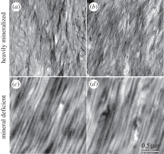
Representative HAADF images of (a,b) heavily mineralized and (c,d) mineral-deficient bone–tendon tissue. In heavily mineralized tissue, collagen fibrils are largely obscured by bioapatite (i.e. the image texture absent in c and d). Note that banded fibrils are barely evident in centre of image (a). Within any given image, brighter image intensity in regions of uniform thickness corresponds to higher mean atomic number. Note that the grey scale ranges for each image have been independently adjusted to enhance visual clarity and are not directly comparable. All images share the same spatial scale.

In heavily mineralized tissue, ubiquitous bioapatite completely obscured mineralized collagen fibrils except in regions that were very thin (less than approx. 50 nm) or suffered mechanical fracture during diamond-knife sectioning. In ultramicrotomy, mechanical fracture of the specimen is a common occurrence, particularly during sectioning of hard or brittle materials. Heavily mineralized tissue broken up by the diamond knife, thereby exposing several mineralized collagen fibrils, was imaged spectrally by STEM–EELS to produce elemental maps. In the EELS elemental maps, Ca (red intensity in figure 3) and C (green intensity in figure 3) can be used as tracers for bioapatite and collagen, respectively. Elemental maps demonstrate that bioapatite is present abundantly throughout mineralized tissue and is concentrated within collagen fibrils in banded segments that repeat periodically along the length of the fibrils (figures 3–6).

Figure 6.

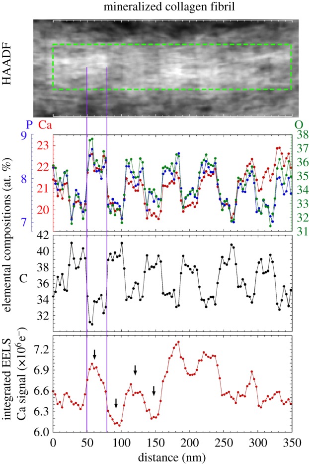
A HAADF image of a mineralized collagen fibril in heavily mineralized tissue is shown at top (brighter contrast corresponds to higher mean atomic number). Column-averaged elemental compositions (in atomic percent) within the mineralized fibril (measured for a region of interest (ROI) highlighted by a green-dotted rectangular box) are shown in the middle two plots. Column-averaged, Ca-L_2,3 signal (integrated over 346.4–391.4 eV, after background subtraction) for the same ROI is shown in the bottom plot. Banded segments within the fibril contain two regions: the first exhibits elevated concentrations of Ca, P and O (indicative of bioapatite) and reduced concentrations of C (indicative of gaps between the N- and C-terminal ends of adjacent collagen molecules); the second region exhibits reduced background concentrations of Ca, P and O and increased concentrations of C (indicative of overlap of collagen molecules). Note that Ca, O and P compositions are spatially correlated and that the Ca/P ratio is approximately constant across the length of the fibril, suggesting a relatively homogeneous bioapatite composition. The ratio of the sum of Ca-L_2,3 signal across two overlap regions to that of the sum of Ca-L_2,3 signal across two gap channels is approximately 0.66. The arrows show the overlap regions and gap channels measured and these appear to have the least amount of extrafibrillar bioapatite present. Vertical lines highlight a gap channel. The analysed region completely overhung a hole in the a-C support film of the TEM grid.

Heavily mineralized tissue regions sufficiently thin to expose collagen fibrils were also imaged by means of STEM–HAADF and STEM–EELS (figures 3–6). Banded regions of the fibrils that exhibited elevated HAADF intensity (i.e. with relatively higher mean atomic number) possessed relatively high concentrations of Ca, P and O (indicative of bioapatite) and significantly reduced concentrations of C (indicative of gaps between the N- and C-terminal ends of adjacent collagen molecules). Similarly, banded regions of low HAADF intensity (i.e. with relatively lower mean atomic number) exhibited the opposite elemental abundance trends. Our results are consistent with coeval STEM observations of elephant ivory (prepared by both focused-ion-beam milling and ultramicrotomy), which is composed primarily of mineralized collagen fibrils [25].

Bands repeat periodically along the length of the fibrils. Their widths are 31.8 ± 0.8 nm (bioapatite-filled gap channel) and 23.0 ± 0.3 nm (region where adjacent collagen molecules overlap) as measured from HAADF images (figure 6). This is consistent with the band-widths 31.8 ± 1.7 nm (bioapatite-filled gap channel) and 23.4 ± 1.7 (collagen molecule overlap region) measured from the FWHM of Ca concentration (i.e. Ca-L_2,3 signal) peaks from EELS profile plots (figure 6). Note that glutaraldehyde-fixation, as performed on our specimens, is known to contract the approximately 67 nm periodicity of the gap + overlap segment [45].

Comparison of elemental EELS profile plots of Ca, P and O to that of C (figure 6) suggest bimodal peaks in bioapatite relative to collagen concentration within the gap channel with peaks located near the gap–overlap boundaries. Furthermore, HAADF images of non-mineralized collagen fibrils in mineral-deficient tissue exhibit increased mean atomic number near the gap–overlap boundaries (figure 7). These features appear associated with topological structures reported for fibrils. Stained fibrils imaged by TEM exhibit a number of sub-bands (or intrabands) within the approximately 67 nm periodic gap–overlap segment [46] with as many as 17 negative-stained bands reported [47]. The bands produced by positive stains mostly correspond to locations within fibrils of charged polar amino acid side chains such as hydroxylysine/arginine and glutamic/aspartic acid, which bind anionic and cationic heavy metals, respectively [48]. The bands produced by negative stains mostly correspond to locations of large hydrophobic amino acid groups [48]. Intrabands are also observed in replicas of freeze-fractured fibrils as depressions and elevations in replica (i.e. specimen) thickness [49], termed X₂, X₃ (located at the gap–overlap transition corresponding to the N-terminal and C-terminal telopeptides, respectively) and X₁ (located in the gap zone) [50]. Subsequent SEM [51] and AFM [51,52] studies confirm these bands are topological ridges on fibrils, and their preservation has been shown to depend on the methods used for specimen preparation [51].

Figure 7.

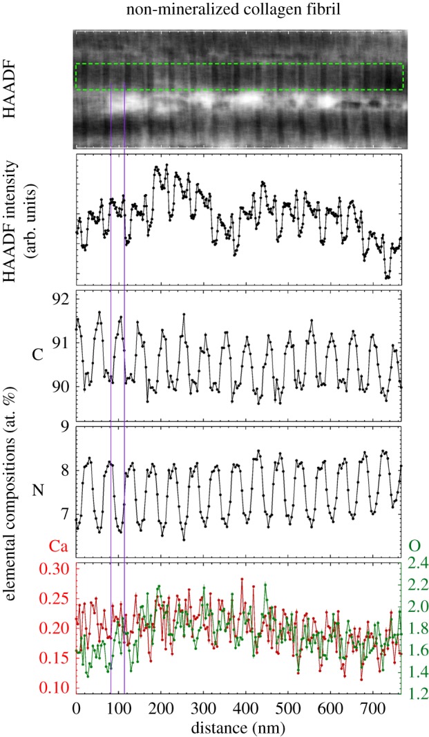
A HAADF image of several laterally adjacent non-mineralized collagen fibrils in mineral-deficient tissue is shown at top (brighter contrast corresponds to higher mean atomic number). Column-averaged HAADF intensity (measured for a ROI highlighted by a green-dotted rectangular box) is shown below. Column-averaged elemental compositions (in atomic per cent) within a non-mineralized fibril for the same ROI are shown in the bottom three plots. Between adjacent fibrils (e.g. just below the ROI) discrete bioapatite grains or small clusters of grains are clearly evident. As shown in the left panel of figure 5, these discrete regions exhibited elevated Ca and O (i.e. bioapatite) and depleted C (i.e. an absence of collagen). The banded segments of the fibrils contain two regions: the first exhibits elevated concentrations of C (indicative of collagen overlap regions) and reduced concentrations of N; the second exhibits reduced concentrations of C (indicative of gaps between the N- and C-terminal ends of adjacent collagen molecules) and elevated concentrations of N. These fibrils exhibited low O concentration, no appreciable Ca concentration, as well as no correlation between the O and trace Ca compositions, indicating no bioapatite was present. In comparison, mineralized fibrils (figure 6) exhibited relatively high O and Ca concentrations that were spatially correlated. The profile plot of the HAADF intensity has twice the pixel resolution as that of the elemental compositions. Vertical lines highlight an overlap region. The analysed region completely overhung a hole in the a-C support film of the TEM grid.

Our STEM–EELS spectra indicate that most of the bioapatite within fibrils is contained within the gap channels. The EELS Ca-L_2,3 signal (integrated over 346.4–391.4 eV of electron energy loss, after background subtraction), column-averaged over a length of a fibril, is shown in figure 6. The integrated Ca-L_2,3 signal represents the number of electrons that were inelastically scattered by Ca atoms within the probed specimen volume (i.e. a STEM image pixel). Assuming constant incident probe current during the course of measurement (which should be the case for our Schottky field emission instrument), the integrated Ca-L_2,3 signal will be proportional to the number of Ca atoms in the probed volume.

The integrated Ca-L_2,3 signal from two overlap regions was summed and likewise the signal from two gap channels was also summed (figure 6) and their ratio 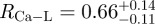was calculated. Assuming the thickness of the cross section was constant over the volume of the fibril where the integrated Ca-L_2,3 signals were summed, R_Ca-L corresponds to the ratio of total mass of bioapatite associated with the overlap regions to that associated with the gap channels. This also assumes the Ca detected in the overlap region is in the form of crystalline bioapatite as opposed to concentrated ions. It is important to note that any extrafibrillar bioapatite present in the cross-sectioned specimen would also contribute to the measured Ca-L_2,3 signal, and hence, R_Ca-L would not necessarily represent the ratio of bioapatite present exclusively within the fibril. Nevertheless, the contribution of the extrafibrillar bioapatite can be modelled and constrained. Assuming a uniform distribution of extrafibrillar bioapatite on the fibrils, the ratio of the intrafibrillar bioapatite within an overlap space, M_O, to intrafibrillar bioapatite within a gap channel, M_G, can be approximated by

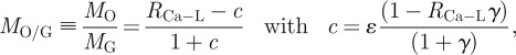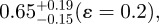
where c is the model correction/conversion term, ɛ is the ratio of extrafibrillar to intrafibrillar bioapatite contributing to the overall Ca-L_2,3 signal (the ratio of the total mass of extrafibrillar bioapatite to the total mass of intrafibrillar bioapatite over the region of integration), and γ  is the ratio of the gap channel volume to the overlap region volume (in the fibril's as-measured state, i.e. not in their physiological setting prior to TEM specimen preparation).  In figure 6, the fibril is exposed for imaging, and consequently, its cross section must contain more collagen fibrillar mass than extrafibrillar mass (i.e. ɛ < 1). Taking γ = 1.4 ± 0.2 (based on STEM–HAADF and EELS measurements), 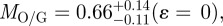or .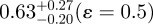

If bioapatite is present predominantly within the collagen fibrils, then, M_O + M_G = 1 or M_O/G= (1−M_G)/M_G (note that M_O and M_G are expressed here and henceforth in units of the fraction of total bioapatite in bone). Our steric model predicts M_G ≤ 0.42 (i.e. 21 vol% upper limit out of a total of 50 vol% of bioapatite in bone) for the fraction of total bioapatite in bone that can be present in the gap channels. Therefore, for the hypothesis that bioapatite is present predominantly within fibrils to be correct, our steric model requires the overlap space must contain at least a factor of M_O/G ≥ 1.38 greater bioapatite than in the gap space. Our STEM–EELS measurement, M_O/G ≤ 0.66, clearly shows that this is not the case. In particular, our steric model and STEM–EELS results constrain the fraction of total bioapatite in bone that is inside fibrils as M_G ≤ 0.42 (i.e. 21 vol% upper limit out of a total 50 vol%) for the gap channels and M_O ≤ 0.28 (i.e. 14 vol% upper limit out of a total 50 vol%) for the intermolecular overlap region. The total intrafibrilar bioapatite is thus constrained as M_O + M_G ≤ 0.7. Therefore, a significant mass of bioapatite (greater than or equal to 0.3 fraction of total bioapatite in bone) must be external to the mineralized fibrils in order to account for the measured volume fraction of bioapatite in bone.

In mineral-deficient tissue, the lack of pervasive bioapatite (compared with that observed in the mineralized regions) allows unobstructed imaging of the collagen fibrils and of extrafibrillar bioapatite within the mineral-deficient tissue (figure 4). In mineral-deficient tissue, discrete bioapatite grains or small clusters of grains were clearly observed outside and between neighbouring collagen fibrils (figure 5). This is most clearly shown in the left panel of figure 5 and in figure 7, where laterally adjacent fibrils are clearly separated and bioapatite occupies the space between the fibrils. The presence of extrafibrillar bioapatite demonstrates that initial bioapatite nucleation and growth may not be confined to intrafibrillar gap channels.

Figure 5.

HAADF images as well as EELS elemental maps showing non-mineralized and mineralized collagen fibrils in mineral-deficient and heavily mineralized tissue, respectively. Ca, O and P intrafibrillar banding are absent in non-mineralized fibrils and present in mineralized fibrils. Bioapatite is evident external to non-mineralized collagen fibrils as localized concentrations of Ca, O and P. Note that the colour ranges for each map are not normalized between 0 at.% and 100 at.% and have been independently adjusted to enhance visual clarity (consequently they are not directly comparable). Grey scale ranges for each HAADF image also have been independently adjusted to enhance visual clarity and are not directly comparable. The analysed regions completely overhung a hole in the a-C support film of the TEM grid.

The collagen fibrils in the mineral-deficient tissue (figure 7), similar to those in heavily mineralized tissue, exhibited bands of elevated concentrations of C (indicative of collagen molecule overlap regions in the microfibrils) that alternated with bands of reduced C (indicative of the gap channels). However, no elevated concentrations of Ca or O (and no correlation in Ca and O concentrations) are observed in the gap channels (or overlap regions) of the mineral-deficient fibrils, indicating the near absence of intrafibrillar bioapatite (note: P was not measured in figure 7). Therefore, data suggest that the mineralization that is present in these tissues developed first in the extrafibrillar space.

The absence of a strong EELS Ca-L_2,3 edge signal whose post-edge tail overlaps with the pre-edge region of the N-K edge signal, allowed quantitative elemental mapping of N in the non-mineralized collagen fibrils (figure 7). Nitrogen is observed concentrated in gap channels of non-mineralized fibrils (at levels greater than which it is present along the entire fibril) present in amines bound to the N-terminus and apparently in other N groups that fill the gap channel. A coeval investigation has also observed N in mineralized fibrils, but its localization was not determined [25]. These N groups may play a role in mineralization, and during mineralization some could be displaced from the gap channel.

In non-mineralized fibrils, fibrillar bands repeat periodically, and their widths are 13.8 ± 0.3 nm (gap channel) and 37.4 ± 0.3 nm (overlap region) as measured from the FWHM of HAADF intensity peaks in profile plots along fibrils. This is consistent with the bandwidths 15.7 ± 0.9 nm (gap channel) and 34.1 ± 1.0 nm (overlap region) measured from the full width C composition peaks in EELS profile plots (figure 7). The non-mineralized fibrils have collagen gap channels that are significantly narrower relative to the overlap regions (ratio ≈ 0.4) than in the case of mineralized fibrils (ratio ≈ 1.4). Unfortunately, no inferences concerning the packing of collagen in fibrils can be drawn from these STEM observations because of the uncertainties in the effects of dehydration and resin infiltration on the fibrils as well as in the degree of possible tissue compression from slicing by the diamond knife. These effects are expected to be more pronounced in non-mineralized collagen than in mineralized collagen structurally reinforced by bioapatite.

As in previous TEM studies, we observed the banding pattern of adjacent collagen fibrils was often correlated and in phase with neighbouring fibrils, suggesting molecular cross-linking between fibrils to maintain that organization during growth. In principle, this architecture would allow bioapatite crystals within the gap space of one collagen fibril to extend over to the gap space of an adjacent fibril. Such bioapatite bridges may very well be present in the heavily mineralized tissue, but visually obscured. Bioapatite is clearly shown both in the gap channels and external to the fibrils; the question is whether these bioapatite grains are fused together to form connected bridges. A number of studies have demonstrated that removal of collagen from bone does not cause the resultant tissue to fall apart [12,53,54]. The presence of extrafibrillar bioapatite may explain this phenomenon if the latter bioapatite formed continuous bridges throughout the tissue. This mechanism and architecture would also explain the observation of bioapatite grains larger than the dimensions of the fibrillar gap channels [28]. Bioapatite bridges, if present, would have significant implications for the bulk mechanical properties of bone.

With any specimen preparation technique, specimen artefacts are a potential concern. Aqueous processing and chemical fixation of bone have been reported to induce structural modification to collagen fibrils as well as to induce some phase transformation, dissolution and reprecipitation of bioapatite [1,13,55]. Of relevance to our results is the question of possible redistribution (i.e. dissolution and reprecipitation) of bioapatite. The effects of this are difficult to assess because the structure and the organization of bioapatite within intermolecular spaces are unknown. Owing to the higher diffusivity offered by the open geometry of the gap channels relative to the more restricted volume of intermolecular space in the overlap region, possible bioapatite dissolution from specimen processing would be expected to occur to a greater extent in the gap channels than in the overlap space. In turn, dissolution of bioapatite in the extrafibrillar volume would be expected to occur to a greater extent than within the fibrils. In fact, AFM studies of collagen fibrils from dentin suggest that the rate of intrafibrillar demineralization is orders of magnitude lower than that of extrafibrillar demineralization [56,57]. These AFM studies also suggest that gap channels are demineralized at a faster rate than overlap regions. Therefore, if ion transport out of the fibrils is not limited, the effects of our TEM specimen preparation would be to skew measurements of M_O/G to larger values than that corresponding to the physiological setting prior to TEM specimen preparation. Therefore, our measurement of M_O/G = 0.66 represents an upper limit for the relative content of bioapatite in the overlap region to that in the gap channels. However, extrafibrillar bioapatite could shield the ingresses to gap channels in many, but not all, TEM cross sections. If extrafibrillar bioapatite effectively shields many of the ingresses to gap channels, redistribution of bioapatite from intrafibrilar and extrafibrilar volumes should be limited. In that case, redistribution of bioapatite within the fibril (i.e. M_O/G ratio) would depend largely on the transport of dissolved ions between the gap channels and intermolecular space. This transport may be significantly limited by the restricted volume of the intermolecular space, as suggested by the AFM studies that show demineralization of the gap space occurs at a faster rate than that of the overlap region [56,57].

Furthermore, it is unlikely that bioapatite dissolution would occur to near completion in some regions of the specimen (i.e. the mineral-deficient tissue) while not in other regions of the same specimen (i.e. heavily mineralized tissue). Therefore, it is reasonable to conclude that the abundant extrafibrillar bioapatite in the heavily mineralized tissue did not result from reprecipitation of bioapatite that dissolved from what became the mineral-deficient tissue.

Variations in bioapatite distribution may exist depending on species, age, anatomical location, remodelling state and other factors. Our studies were performed on adult rat humeral heads and are relevant to that specific tissue and timepoint. Our ongoing studies are examining the effect of age (neonatal through adult) and location (from unmineralized tendon to fully mineralized bone) in mouse shoulders.

3.3. Mechanical implications of bone's nanophysiology

Stiffening and toughening mechanisms of biological tissues are governed by their nanophysiology [58]. From the perspective of stiffness, placement of bioapatite only in gap channels (in series with collagen) is the least effective strategy for stiffening bone [59]. However, extrafibrillar bioapatite would stiffen bone significantly by forming a concentric shell or interconnected network surrounding and (through aligned gap channels) interpenetrating collagen fibrils [60], increasing axial stiffness and especially flexural stiffness when the bioapatite network percolates [59]. Addition of bioapatite in fibril overlap regions (i.e. intermolecular spaces) would also stiffen the nanocomposite structure if a continuous bioapatite network formed. However, geometric constraints within the intermolecular space, as represented by Orgel et al. [6,7], may limit structural interconnections of bioapatite. On the other hand, fibril overlap regions that lack a continuous bioapatite network could serve a different function, perhaps absorbing energy and deflecting growing cracks. A similar mechanism has been proposed for compliant fibril–fibril connections based on AFM studies [61]. The specific arrangement of bioapatite with respect to collagen also has implications for fracture toughness [62]. This concept is consistent with the simulations of Buehler et al. [58] showing that tissue toughness can be optimized by an intermediate degree of cross-linking. The intermediate between a stiffening brittle sheath and a toughening energy-absorbing barrier is analogous to the trade-off in the design of fibrous composite materials [63,64]: in both cases, the goal is a stiff material that shields fibres from cracks through an energy-absorbing sacrificial layer.

4. Conclusions

We mapped the volumetric distribution of bioapatite within the structure of bone using steric modelling and STEM–EELS. Our results demonstrate that a significant fraction of bioapatite (greater than 30%) exists external to collagen fibrils. Our steric model predicts that gap channels can accommodate up to 42 per cent of the total bioapatite within bone. While the specific quantity and organization of bioapatite within intermolecular spaces remains elusive, our STEM–EELS measurements suggest that the volume of bioapatite contained within intermolecular spaces of overlap regions is approximately 2/3 that contained within gap channels. We also conclude that not only is there a significant amount of extrafibrillar mineralization, but that such mineralization can occur before and even in the absence of the long-recognized intrafibrillar mineralization.

References

- 1.Glimcher M. J. 2006. Bone: nature of the calcium phosphate crystals and cellular, structural, and physical chemical mechanisms in their formation. Rev. Mineral. Geochem. 64, 223–282 10.2138/rmg.2006.64.8 (doi:10.2138/rmg.2006.64.8) [DOI] [Google Scholar]
- 2.Hollister D. W. 1987. Molecular basis of osteogenesis imperfecta. Curr. Probl. Dermatol. 17, 76–94 [DOI] [PubMed] [Google Scholar]
- 3.Boskey A. 2001. Bone mineralization. In Bone mechanics handbook, 2nd edn. (ed. Cowin S. C.), p. 5:1–33 Boca Raton, FL: CRC Press [Google Scholar]
- 4.Hodge A. J., Petruska J. A. 1963. In Aspects of protein structure (ed. Ramachandran G. N.), pp. 289–300 New York, NY: Academic Press [Google Scholar]
- 5.Landis W. J., Moradian-Oldak J., Weiner S. 1991. Topographic imaging of mineral and collagen in the calcifying turkey tendon. Connect. Tissue Res. 25, 181–196 10.3109/03008209109029155 (doi:10.3109/03008209109029155) [DOI] [PubMed] [Google Scholar]
- 6.Orgel J. P. R. O., Miller A., Irving T. C., Fischetti R. F., Hammersley A. P., Wess T. J. 2001. The in situ supermolecular structure of type I collagen. Structure 9, 1061–1069 10.1016/S0969-2126(01)00669-4 (doi:10.1016/S0969-2126(01)00669-4) [DOI] [PubMed] [Google Scholar]
- 7.Orgel J. P. R. O., Irving T. C., Miller A., Wess T. J. 2006. Microfibrillar structure of type I collagen in situ. Proc. Natl Acad. Sci. USA 103, 9001–9005 10.1073/pnas.0502718103 (doi:10.1073/pnas.0502718103) [DOI] [PMC free article] [PubMed] [Google Scholar]
- 8.Landis W. J., Song M. J., Leith A., McEwen L., McEwen B. F. 1993. Mineral and organic matrix interaction in normally calcifying tendon visualized in three dimensions by high-voltage electron microscopic tomography and graphic image reconstruction. J. Struct. Biol. 110, 39–54 10.1006/jsbi.1993.1003 (doi:10.1006/jsbi.1993.1003) [DOI] [PubMed] [Google Scholar]
- 9.Hodge A. J. 1967. Structure at the electron microscopic level. In Treatise on collagen (ed. Ramachandran G.), pp. 185–205 New York, NY: Academic Press [Google Scholar]
- 10.Hodge A. J. 1989. Molecular models illustrating the possible distributions of ‘holes’ in simple systematically staggered arrays of type I collagen molecules in native-type fibrils. Connect. Tissue Res. 21, 137–147 10.3109/03008208909050004 (doi:10.3109/03008208909050004) [DOI] [PubMed] [Google Scholar]
- 11.Katz E. P., Li S. T. 1973. Structure and function of bone collagen fibrils. J. Mol. Biol. 80, 1–15 10.1016/0022-2836(73)90230-1 (doi:10.1016/0022-2836(73)90230-1) [DOI] [PubMed] [Google Scholar]
- 12.Olszta M. J., Cheng X., Jee S. S., Kumar R., Kim Y. Y., Kaufman M. J., Douglas E. P., Gower L. B. 2007. Bone structure and formation: a new perspective. Mater. Sci. Eng. R-Rep. 58, 77–116 10.1016/j.mser.2007.05.001 (doi:10.1016/j.mser.2007.05.001) [DOI] [Google Scholar]
- 13.Landis W. J., Hauschka B. T., Rogerson C. A., Glimcher M. J. 1977. Electron microscopic observations of bone tissue prepared by ultracryomicrotomy. J. Ultrastruct. Res. 59, 185–206 10.1016/S0022-5320(77)80079-8 (doi:10.1016/S0022-5320(77)80079-8) [DOI] [PubMed] [Google Scholar]
- 14.Lee D. D., Glimcher M. J. 1991. Three-dimensional spatial relationship between the collagen fibrils and the inorganic calcium phosphate crystals of pickerel (Americanus americanus) and herring (Clupea harengus) bone. J. Mol. Biol. 217, 487–501 10.1016/0022-2836(91)90752-R (doi:10.1016/0022-2836(91)90752-R) [DOI] [PubMed] [Google Scholar]
- 15.Glimcher M. J. 1959. Molecular biology of mineralized tissues with particular reference to bone. Rev. Mod. Phys. 31, 359–393 10.1103/RevModPhys.31.359 (doi:10.1103/RevModPhys.31.359) [DOI] [Google Scholar]
- 16.Glimcher M. J. 1968. A basic architectural principle in the organization of mineralized tissues. In Proc 5th European Symp. Calcif Tiss (ed. Milhaud G., Owen M., Blackwood H. J. J.), pp. 3–26 Paris: Societe d'Edition d'Enseignement Superieur; [PubMed] [Google Scholar]
- 17.White S. W., Hulmes D. J. S., Miller A., Timmins P. A. 1977. Collagen–mineral axial relationship in calcified turkey leg tendon by X-ray and neutron diffraction. Nature 266, 421–425 10.1038/266421a0 (doi:10.1038/266421a0) [DOI] [PubMed] [Google Scholar]
- 18.Miller A. 1984. Collagen: the organic matrix in bone. In Mineral phases in biology (ed. Miller A., Phillips D., Williams R. J. P.), pp. 45–68 London, UK: Royal Society [Google Scholar]
- 19.Berthet-Colominas C., Miller A., White S. W. 1979. Structural study of the calcifying collagen in turkey leg tendons. J. Mol. Biol. 134, 431–445 10.1016/0022-2836(79)90362-0 (doi:10.1016/0022-2836(79)90362-0) [DOI] [PubMed] [Google Scholar]
- 20.Bonar L. C., Lees S., Mook H. A. 1985. Neutron diffraction studies of collagen in fully mineralized bone. J. Mol. Biol. 181, 265–270 10.1016/0022-2836(85)90090-7 (doi:10.1016/0022-2836(85)90090-7) [DOI] [PubMed] [Google Scholar]
- 21.Fraser R. D. B., MacRae T. P., Miller A., Suzuki E. 1983. Molecular conformation and packing in collagen fibrils. J. Mol. Biol. 167, 497–521 10.1016/S0022-2836(83)80347-7 (doi:10.1016/S0022-2836(83)80347-7) [DOI] [PubMed] [Google Scholar]
- 22.Berthet-Colominas C., Miller A., Herbage D., Ronziere M. C., Tocchetti D. 1982. Structural studies of collagen fibers from intervertebral disk. Biochim. Biophys. Acta 706, 50–64 10.1016/0167-4838(82)90374-0 (doi:10.1016/0167-4838(82)90374-0) [DOI] [PubMed] [Google Scholar]
- 23.Landis W. J., Hodgens K. J., Song M. J., Arena J., Kiyonaga S., Marko M., Owen C., McEwen B. F. 1996. Mineralization of collagen may occur on fibril surfaces: evidence from conventional and high-voltage electron microscopy and three-dimensional imaging. J. Struct. Biol. 117, 24–35 10.1006/jsbi.1996.0066 (doi:10.1006/jsbi.1996.0066) [DOI] [PubMed] [Google Scholar]
- 24.Landis W. J., Song M. J. 1991. Early mineral deposition in calcifying tendon characterized by high voltage electron microscopy and 3-dimensional graphic imaging. J. Struct. Biol. 107, 116–127 10.1016/1047-8477(91)90015-O (doi:10.1016/1047-8477(91)90015-O) [DOI] [PubMed] [Google Scholar]
- 25.Jantou-Morris V., Horton M. A., McComb D. W. 2010. The nano-morphological relationships between apatite crystals and collagen fibrils in ivory dentine. Biomaterials 31, 5275–5286 10.1016/j.biomaterials.2010.03.025 (doi:10.1016/j.biomaterials.2010.03.025) [DOI] [PubMed] [Google Scholar]
- 26.Lees S., Prostak K. 1988. The locus of mineral crystallites in bone. Connect. Tissue Res. 18, 41–54 10.3109/03008208809019071 (doi:10.3109/03008208809019071) [DOI] [PubMed] [Google Scholar]
- 27.Lees S., Prostak K. S., Ingle V. K., Kjoller K. 1994. The loci of mineral in turkey leg tendon as seen by atomic force microscope and electron microscopy. Calcif. Tissue Int. 55, 180–189 10.1007/BF00425873 (doi:10.1007/BF00425873) [DOI] [PubMed] [Google Scholar]
- 28.Hassenkam T., Fantner G. E., Cutroni J. A., Weaver J. C., Morse D. E., Hansma P. K. 2004. High-resolution AFM imaging of intact and fractured trabecular bone. Bone 35, 4–10 10.1016/j.bone.2004.02.024 (doi:10.1016/j.bone.2004.02.024) [DOI] [PubMed] [Google Scholar]
- 29.Sasaki N., Tagami A., Goto T., Taniguchi M., Nakata M., Hikichi K. 2002. Atomic force microscopic studies on the structure of bovine femoral cortical bone at the collagen fibril–mineral level. J. Mater. Sci. Mater. Med. 13, 333–337 10.1023/A:1014079421895 (doi:10.1023/A:1014079421895) [DOI] [PubMed] [Google Scholar]
- 30.Pidaparti R. M. V., Chandran A., Takano Y., Turner C. H. 1996. Bone mineral lies mainly outside collagen fibrils: predictions of a composite model for osteonal bone. J. Biomech. 29, 909–916 10.1016/0021-9290(95)00147-6 (doi:10.1016/0021-9290(95)00147-6) [DOI] [PubMed] [Google Scholar]
- 31.Alexander B. E., Daulton T. L., Genin G. M., Pasteris J. D., Wopenka B., Thomopoulos S. 2009. The nano-physiology of mineralized tissues. In Proc. of the ASME 2009 Summer Bioengineering Conf. (SBC2009), p.175 New York, NY: American Society of Mechanical Engineer [Google Scholar]
- 32.Egerton R. F. 1996. Electron energy-loss spectroscopy in the electron microscope. New York, NY: Plenum [Google Scholar]
- 33.Hughes J. M., Cameron M., Crowley K. D. 1990. Crystal-structures of natural ternary apatites: solid solution in the Ca5(PO4)3X (X = F, OH, Cl) system. Am. Mineral. 75, 295–304 [Google Scholar]
- 34.McConnell D. 1973. Apatite: its crystal chemistry, mineralogy, utilization, and geologic and biologic occurrences. New York, NY: Springer [Google Scholar]
- 35.Nriagu J. O., Moore P. B. 1984. Phosphate minerals. New York, NY: Springer [Google Scholar]
- 36.Hughes J. M., Rakovan J. 2002. The crystal structure of apatite, Ca5(PO4)3(F,OH,Cl). In Phosphates: geochemical, geobiological and material importance reviews in mineralogy and geochemistry (eds Kohn M. J., Rakovan J., Hughes J. M.), pp. 1–12 Washington, DC: Mineralogical Society of America [Google Scholar]
- 37.Pan Y., Fleet M. E. 2002. Compositions of the apatite-group minerals: Substitution mechanisms and controlling factors. In Phosphates: geochemical, geobiological and material importance reviews in mineralogy and geochemistry (eds Kohn D. H., Rakovan J., Hughes J. M.), pp. 13–50 Washington, DC: Mineralogical Society of America [Google Scholar]
- 38.Cazalbou S., Combes C., Eichert D., Rey C. 2004. Adaptative physico-chemistry of bio-related calcium phosphates. J. Mater. Chem. 14, 2148–2153 10.1039/B401318b (doi:10.1039/B401318b) [DOI] [Google Scholar]
- 39.Eppell S. J., Tong W., Katz J. L., Kuhn L., Glimcher M. J. 2001. Shape and size of isolated bone mineralites measured using atomic force microscopy. J. Orthop. Res. 19, 1027–1034 10.1016/S0736-0266(01)00034-1 (doi:10.1016/S0736-0266(01)00034-1) [DOI] [PubMed] [Google Scholar]
- 40.Tong W., Glimcher M. J., Katz J. L., Kuhn L., Eppell S. J. 2003. Size and shape of mineralites in young bovine bone measured by atomic force microscopy. Calcif. Tissue Int. 72, 592–598 10.1007/s00223-002-1077-7 (doi:10.1007/s00223-002-1077-7) [DOI] [PubMed] [Google Scholar]
- 41.Derwin K. A., Soslowsky L. J. 1999. A quantitative investigation of structure–function relationships in a tendon fascicle model. J. Biomech. Eng. 121, 598–604 10.1115/1.2800859 (doi:10.1115/1.2800859) [DOI] [PubMed] [Google Scholar]
- 42.Fratzl P., Fratzl-Zelman N., Klaushofer K. 1993. Collagen packing and mineralization. An x-ray scattering investigation of turkey leg tendon. Biophys. J. 64, 260–266 10.1016/S0006-3495(93)81362-6 (doi:10.1016/S0006-3495(93)81362-6) [DOI] [PMC free article] [PubMed] [Google Scholar]
- 43.Arsenault A. L. 1989. A comparative electron microscopic study of apatite crystals in collagen fibrils of rat bone, dentin and calcified turkey leg tendons. Bone Mineral 6, 165–177 10.1016/0169-6009(89)90048-2 (doi:10.1016/0169-6009(89)90048-2) [DOI] [PubMed] [Google Scholar]
- 44.Maitland M. E., Arsenault A. L. 1991. A correlation between the distribution of biological apatite and amino acid sequence of type I collagen. Calcif. Tissue Int. 48, 341–352 10.1007/BF02556154 (doi:10.1007/BF02556154) [DOI] [PubMed] [Google Scholar]
- 45.Ortolani F., Marchini M. 1995. Cartilage type II collagen fibrils show distinctive negative-staining band patterns differences between type II and type I unfixed or glutaraldehyde-fixed collagen fibrils. J. Electron Microsc. 44, 365–375 [PubMed] [Google Scholar]
- 46.Schmitt F. O., Gross J. 1948. Further progress in the electron microscopy of collagen. J. Am. Leather Chem. Assoc. 43, 658–675 [Google Scholar]
- 47.Shinagawa Y., Shinagawa Y. 1974. Studies on collagen fibrils in amphibian skin by means of thin sectioning and densitometric method. J. Electron Microsc. 23, 161–165 [PubMed] [Google Scholar]
- 48.Kobayashi K., Ito T., Hoshino T. 1986. Correlation between negative staining pattern and hydrophobic residues of collagen. J. Electron Microsc. 35, 272–275 [PubMed] [Google Scholar]
- 49.Marchini M., Morocutti M., Castellani P. P., Leonardi L., Ruggeri A. 1983. The banding pattern of rat tail tendon freeze-etched collagen fibrils. Connect. Tissue Res. 11, 175–184 10.3109/03008208309004853 (doi:10.3109/03008208309004853) [DOI] [PubMed] [Google Scholar]
- 50.Bairati A., Petruccioli M. G., Tarelli L. T. 1969. Studies on the ultrastructure of collagen fibrils. 1. Morphological evaluation of the periodic structure. J. Submicrosc. Cytol. 1, 113–141 [Google Scholar]
- 51.Raspanti M., Alessandrini A., Gobbi P., Ruggeri A. 1996. Collagen fibril surface: TMAFM, FEG-SEM and freeze-etching observations. Microsc. Res. Tech. 35, 87–93 (doi:10.1002/(SICI)1097-0029(19960901)35:1<87::AID-JEMT8>3.0.CO;2-P) [DOI] [PubMed] [Google Scholar]
- 52.Baselt D. R., Revel J. P., Baldeschwieler J. D. 1993. Subfibrillar structure of type I collagen observed by atomic force microscopy. Biophys. J. 65, 2644–2655 10.1016/S0006-3495(93)81329-8 (doi:10.1016/S0006-3495(93)81329-8) [DOI] [PMC free article] [PubMed] [Google Scholar]
- 53.Rosen V. B., Hobbs L. W., Spector M. 2002. The ultrastructure of anorganic bovine bone and selected synthetic hyroxyapatites used as bone graft substitute materials. Biomaterials 23, 921–928 10.1016/S0142-9612(01)00204-6 (doi:10.1016/S0142-9612(01)00204-6) [DOI] [PubMed] [Google Scholar]
- 54.Chen P. Y., Toroian D., Price P. A., McKittrick J. 2011. Minerals form a continuum phase in mature cancellous bone. Calcif. Tissue Int. 88, 351–361 10.1007/s00223-011-9462-8 (doi:10.1007/s00223-011-9462-8) [DOI] [PMC free article] [PubMed] [Google Scholar]
- 55.Boothroyd B. 1964. The problem of demineralisation in thin sections of fully calcified bone. J. Cell Biol. 20, 165–173 10.1083/jcb.20.1.165 (doi:10.1083/jcb.20.1.165) [DOI] [PMC free article] [PubMed] [Google Scholar]
- 56.Balooch M., Balooch G., Habelitz S., Marshall S. J., Marshall G. W. 2004. Intrafibrillar demineralization study of single human dentin collagen fibrils by AFM. Mat. Res. Soc. Symp. Proc. 823, W6.1 10.1557/PROC-823-W6.1 (doi:10.1557/PROC-823-W6.1) [DOI] [Google Scholar]
- 57.Balooch M., Habelitz S., Kinney J. H., Marshall S. J., Marshall G. W. 2008. Mechanical properties of mineralized collagen fibrils as influenced by demineralization. J. Struct. Biol. 162, 404–410 10.1016/j.jsb.2008.02.010 (doi:10.1016/j.jsb.2008.02.010) [DOI] [PMC free article] [PubMed] [Google Scholar]
- 58.Buehler M. J. 2007. Molecular nanomechanics of nascent bone: fibrillar toughening by mineralization. Nanotechnology 18, 295102 10.1088/0957-4484/18/29/295102 (doi:10.1088/0957-4484/18/29/295102) [DOI] [Google Scholar]
- 59.Genin G. M., Kent A., Birman V., Wopenka B., Pasteris J. D., Marquez P. J., Thomopoulos S. 2009. Functional grading of mineral and collagen in the attachment of tendon to bone. Biophys. J. 97, 976–985 10.1016/j.bpj.2009.05.043 (doi:10.1016/j.bpj.2009.05.043) [DOI] [PMC free article] [PubMed] [Google Scholar]
- 60.Katz E. P., Wachtel E., Yamauchi M., Mechanic G. L. 1989. The structure of mineralized collagen fibrils. Connect. Tissue Res. 21, 149–154 (discussion 55–58) 10.3109/03008208909050005 (doi:10.3109/03008208909050005) [DOI] [PubMed] [Google Scholar]
- 61.Fantner G. E., et al. 2005. Sacrificial bonds and hidden length dissipate energy as mineralized fibrils separate during bone fracture. Nat. Mater. 4, 612–616 10.1038/nmat1428 (doi:10.1038/nmat1428) [DOI] [PubMed] [Google Scholar]
- 62.Jager I., Fratzl P. 2000. Mineralized collagen fibrils: a mechanical model with a staggered arrangement of mineral particles. Biophys. J. 79, 1737–1746 10.1016/S0006-3495(00)76426-5 (doi:10.1016/S0006-3495(00)76426-5) [DOI] [PMC free article] [PubMed] [Google Scholar]
- 63.Genin G. M., Hutchinson J. W. 1997. Composite laminates in plane stress: constitutive modeling, and stress redistribution due to matrix cracking. J. Am. Ceram. Soc. 80, 1245–1255 10.1111/j.1151-2916.1997.tb02971.x (doi:10.1111/j.1151-2916.1997.tb02971.x) [DOI] [Google Scholar]
- 64.Budiansky B., Hutchinson J. W., Evans A. G. 1986. Matrix fracture in fiber-reinforced ceramics. J. Mech. Phys. Solids 34, 167–189 10.1016/0022-5096(86)90035-9 (doi:10.1016/0022-5096(86)90035-9) [DOI] [Google Scholar]