Motion correction for phase-resolved dynamic optical coherence tomography imaging of rodent cerebral cortex

Abstract

Cardiac and respiratory motions in animals are the primary source of image quality degradation in dynamic imaging studies, especially when using phase-resolved imaging modalities such as spectral-domain optical coherence tomography (SD-OCT), whose phase signal is very sensitive to movements of the sample. This study demonstrates a method with which to compensate for motion artifacts in dynamic SD-OCT imaging of the rodent cerebral cortex. We observed that respiratory and cardiac motions mainly caused, respectively, bulk image shifts (BISs) and global phase fluctuations (GPFs). A cross-correlation maximization-based shift correction algorithm was effective in suppressing BISs, while GPFs were significantly reduced by removing axial and lateral global phase variations. In addition, a non-origin-centered GPF correction algorithm was examined. Several combinations of these algorithms were tested to find an optimized approach that improved image stability from 0.5 to 0.8 in terms of the cross-correlation over 4 s of dynamic imaging, and reduced phase noise by two orders of magnitude in ~8% voxels.

1. Introduction

Optical coherence tomography (OCT) has provided an unprecedented tool for label-free structural imaging of biological systems [1]. In particular, spectral-domain optical coherence tomography (SD-OCT) enables measurement of the phase of light reflected from tissue [2,3]. Applications of OCT have recently expanded to include dynamic imaging of biological specimens to study how the optical property of tissue varies in time, from in vitro single cells [4,5] to in vivo brain tissue [6,7], and from measuring baseline dynamics [4,6] to exploring temporal variations associated with environmental interactions [5,7].

Generally, in in vivo dynamic imaging, heartbeat and breathing are the primary source of image quality degradation. As the phase of the SD-OCT signal is very sensitive to sample movements, these cardiac and respiratory motions of the animal cause especially high noise in dynamic SD-OCT imaging. For example, a 1-μm axial movement produces a large fluctuation of ~10 rad in the phase of the OCT signal when the center wavelength of the light source is 1300 nm. Such motion-oriented noise becomes particularly problematic in studies monitoring biological systems for a relatively long time (longer than several cycles of cardiac/respiratory motions). Therefore, motion correction processing is one of the most important steps in analyzing such long-term dynamic imaging data (e.g., when recording temporal responses of the brain to functional activation).

Motion correction algorithms have been studied across various modalities, including functional magnetic resonance imaging (fMRI) [8,9], positron emission tomography (PET) [10,11], emission computed tomography (ECT) [12], optical cardiac/ophthalmic imaging [13–17] and structural OCT imaging [18,19]. Most of these studies have employed external systems such as optical motion tracking systems [8–12, 16,17] or motion-gating electronics [15]. In contrast, in this paper we propose a motion correction method that requires no external aid and is especially suitable for phase-resolved dynamic OCT imaging.

To this end, we hypothesize that respiratory and cardiac motions will mainly cause, respectively, bulk image shifts (BISs) and global phase fluctuations (GPFs); a cross-correlation maximization-based method will be effective for BIS compensation; GPFs will be suppressed by removing phase variations that are global in either the axial or the lateral direction; and an appropriate combination of BIS and GPF correction algorithms will sufficiently suppress motion artifacts. To confirm these hypotheses, we acquired dynamic imaging data from the rodent cerebral cortex using our SD-OCT system, characterized motion-oriented noises, examined several algorithms to suppress those motion artifacts, and tested the performance of different combinations of algorithms.

2. Materials and experimental methods

2.1 Animal preparation

Sprague Dawley rats (250-300 g) were initially anesthetized with isofluorane (1.5-2.5%, v/v), and ventilated with a mixture of air and oxygen during surgical procedures. Tracheotomy and cannulation of the femoral artery and vein were done. Following this, the head was fixed in a stereotaxic frame, and the scalp retracted. Craniotomy was performed using a saline-cooled dental drill and a 3 mm × 3 mm area over the somatosensory cortex was exposed. The dura was carefully removed, and then the brain surface was covered with agarose gel and a glass cover slip and sealed with dental acrylic cement. After surgery, rats were anesthetized with a mixture of ketamine-xylazine (20 mg/kg/hr - 2 mg/kg/hr, i.v.) and moved to our OCT system for experiment. Physiological signs such as heart rate, body temperature and blood pressure were continuously monitored during surgery and during the experiment. All experimental procedures were approved by the Massachusetts General Hospital Subcommitee on Research Animal Care.

2.2 Spectral-domain optical coherence tomography system for in vivo brain imaging

We used an SD-OCT system (Thorlabs, Inc) optimized for in vivo dynamic imaging of the rodent cerebral cortex as described in a previous publication [6] (Fig. 1A ). We employed a large-bandwidth near-infrared light source for a large imaging depth and high spatial resolution. The light source consisted of two superluminescent diodes to yield 170-nm bandwidth centered at 1310 nm, enabling an axial resolution of 3.5 μm in tissue. Light reflected from the reference mirror and from the sample interfered via a 50/50 fiber coupler. The spectrum of interfered light was measured with a 1024 pixel InGaAs line scan camera at 47,000 spectra/s. A 5 × objective was used, enabling a transverse resolution of 7 μm in tissue. The surface of the cortex was illuminated by another light source, with a wavelength of 570 ± 5 nm, so the cortical surface was simultaneously imaged by using a CCD (Fig. 1B).

Fig. 1.

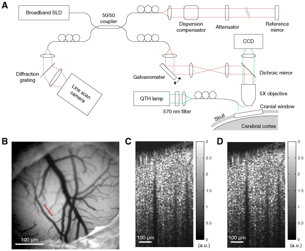
(A) Schematics of the SD-OCT system for in vivo brain imaging. (B) Image of the surface of the rodent cerebral cortex obtained by the CCD. The white scale bar indicates 1 mm. The red line indicates the scanning line of OCT imaging. (C) The intensity map of OCT shows a depth-resolved tissue structure of the cross-sectional area indicated by the red line in (B). The intensity map was averaged over 1000 frames (4 s). (D) The noise map from dynamic OCT imaging. This noise map looks very similar to the intensity map because the phase fluctuation exceeded 2π.

2.3 Dynamic imaging and data processing

A cross-section of the cortex was repeatedly scanned with our OCT system. The positions of the reference mirror and the objective lens were adjusted to enhance focus as well as to minimize the intrusion of the reflection from the glass cover slip into the tissue area. The cross-sectional area contained 96 axial scans, resulting in a frame rate of 250 area/s. The area was scanned one thousand times in four seconds. The spectrum data were Fourier-transformed to spatial data of OCT signals proportional to the complex-valued field-reflectivity of tissue. A map of the magnitude of the OCT signal (intensity map) showed the depth-resolved tissue structure of the cerebral cortex (Fig. 1C). A map of the standard deviation of the OCT signal (noise map) is presented in Fig. 1D.

3. Algorithms and results

3.1 Image shift and global phase fluctuations due to cardiac and respiratory motion

Physiological fluctuations were observed in the dynamic OCT imaging due to cardiac and respiratory motions of the animal. In addition to these physiological fluctuations, environmental vibrations and/or jittering in the galvanometer operation may cause fluctuations that are common across voxels. These fluctuations, however, turned out to be much smaller than the physiological fluctuations.

We used a cross-correlation as an index of image stability.

$$\Gamma (t)=\frac{{\displaystyle \int R(z,x,t)R^{*}(z,x,t_0)dzdx}}{\sqrt{{\displaystyle \int {\left|R(z,x,t)\right|}^{2}dzdx}}\sqrt{{\displaystyle \int {\left|R(z,x,t_0)\right|}^{2}dzdx}}}$$ (1)

where R(z,x,t) is the complex-valued OCT signal, and R*(z,x,t₀) is the complex conjugate of R(z,x,t) at the reference time t₀. Here, we chose the first frame as the reference, that is, t₀ = 0. The magnitude of this cross-correlation, |Γ(t)|, quantifies the similarity between the reference frame and a frame acquired at time t. We also monitored the absolute real part of the cross-correlation, |Re[Γ(t)]|, because this is more sensitive to changes in the phase of OCT signals. As can be seen in Fig. 2A , we observed two types of dips in the cross-correlation: large and low-frequency ones, and smaller but high-frequency ones. These might be attributed to image decorrelation caused by respiratory and cardiac motions, respectively. Frequencies of each decorrelation (0.9 and 6.5 Hz) matched well with those of the respiration and heartbeat of the animal. This decorrelation may be caused by a bulk image shift and/or global fluctuations in the phase of the OCT signal. These two origins of decorrelation might be coupled to one another, because a sub-pixel shift of the sample may cause a global change in the phase of the OCT signals. Examples of the GPF are shown in Fig. 2B. Phase fluctuations were global not only in the axial direction but also in the lateral direction.

Fig. 2.

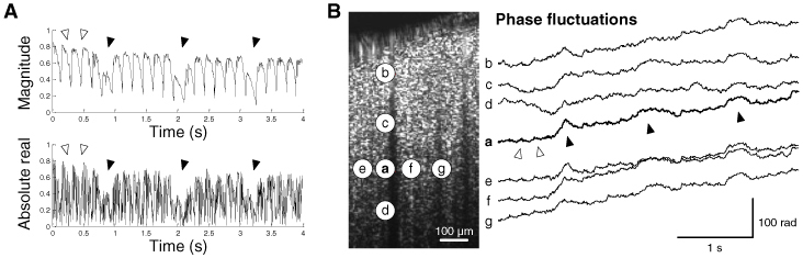
Motion artifacts in dynamic OCT imaging. (A) The magnitude and absolute real part of the cross-correlation. Filled arrows indicate low-frequency decorrelation due to respiratory motions, while empty arrows indicate high-frequency decorrelation due to cardiac motions. (B) Example voxels showing axial and lateral global fluctuations in the phase of OCT signals. Axial global phase fluctuations were observed across voxels a-d, while lateral global fluctuations were observed across voxels a and e-g. Large phase increases due to respiratory motions (filled arrows) were observed across voxels located at the identical depth (voxels a, e, f, and g). Phases were unwrapped in the temporal direction.

3.2 Correction of image shift

A shift in the image can be found by maximizing the cross-correlation of shifted images to the reference frame. Cross-correlations for various shifts were obtained at each frame by using Eq. (2).

$${\Gamma }_{shift}(\Delta z,\Delta x,t)=\frac{\left|{\displaystyle \int R(z+\Delta z,x+\Delta x,t)R^{*}(z,x,t_0)dzdx}\right|}{\sqrt{{\displaystyle \int {\left|R(z+\Delta z,x+\Delta x,t)\right|}^{2}dzdx}}\sqrt{{\displaystyle \int {\left|R(z,x,t_0)\right|}^{2}dzdx}}}$$ (2)

where R(z,x,t) is the complex-valued OCT signal, and R*(z,x,t₀) is the complex conjugate of R(z,x,t) at the reference time t₀. The first step in finding sub-pixel shifts was upsampling of images with the cubic spline interpolation. Shifts found in each upsampled image were compensated for, and then the image was downsampled to its original sampling. In this study, images were four-fold upsampled, which means sub-pixel shifts down to 1/4 pixel could be detected.

As a result, axial and lateral shifts of the images were found and compensated for (Fig. 3A ). The axial shift was large when the animal made respiratory motions. Compensation reduced respiration-oriented large dips in the cross-correlation (Fig. 3B). In contrast, this BIS correction provided little enhancement to the absolute real part of cross-correlation, which is more sensitive to phase fluctuations. The ratio of noise of motion-corrected data to that of raw data was calculated at every voxel. As can be seen in the population of this noise reduction ratio (NRR, Fig. 3C), 61.7% of the voxels showed a decrease in the noise as a result of BIS correction. This small population of enhanced voxels is due to the fact that the BIS correction was not effective in reducing phase noise.

Fig. 3.

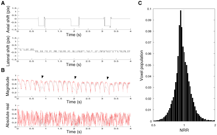
Effects of BIS correction. (A) Sub-pixel axial and lateral shifts of the image obtained by maximizing the cross-correlation magnitude. Shifts were presented in pixels. (B) The cross-correlation of BIS-corrected images. Amplitudes of respiration-oriented dips (filled arrows) were reduced to be similar to those of cardiac motion-oriented dips. The gray line shows the cross-correlation of raw data. (C) Normalized population of the noise reduction ratio.

3.3 Correction of global phase fluctuation

Cardiac and respiratory motions also caused fluctuations in the phase of the OCT signal. Those phase fluctuations were commonly observed across voxels in both the axial and the lateral directions (Fig. 2B). Axial global phase fluctuations (AGPFs) were determined at each lateral position and time such that the real part of the cross-correlation of the phase-shifted frame to the reference frame (Eq. (3) was maximized.

$$\mathrm{Re}\left[{\Gamma }_{phase}(x,t;AGPF(x,t))\right]=\frac{\mathrm{Re}\left[{\displaystyle \int R(z,x,t)e^{iAGPF(x,t)}{R}^{*}(z,x,t_0)dz}\right]}{\sqrt{{\displaystyle \int {\left|R(z,x,t)\right|}^{2}dz}}\sqrt{{\displaystyle \int {\left|R(z,x,t_0)\right|}^{2}dz}}}$$ (3)

Since the AGPF is independent of z, it can be directly obtained by Eq. (4).

$$AGPF(x,t)=-\arg \left[{\displaystyle \int R(z,x,t)R^{*}(z,x,t_0)dz}\right]$$ (4)

Similarly, lateral global phase fluctuations (LGPFs) can be obtained at each depth and time by Eq. (5).

$$LGPF(z,t)=-\arg \left[{\displaystyle \int R(z,x,t)R^{*}(z,x,t_0)dx}\right]$$ (5)

As shown in Fig. 4A , cardiac and respiratory motion-oriented fluctuations were clearly observed in both AGPF and LGPF. When both GPFs were compensated for, amplitudes of cardiac motion-oriented dips were remarkably reduced, whereas the effect on respiration-oriented dips was small (Fig. 4B). This result might be attributed to the fact that respiratory motions produced BISs larger than the size of pixel (Fig. 3A), so the GPF correction alone cannot compensate such supra-pixel movements. It is worth noting that the absolute real part was identical to the magnitude because the GPF correction makes the cross-correlation a real value (Eq. (3). Compared to the BIS correction, many more voxels (95.5%) showed a decrease in the noise (Fig. 4C).

Fig. 4.

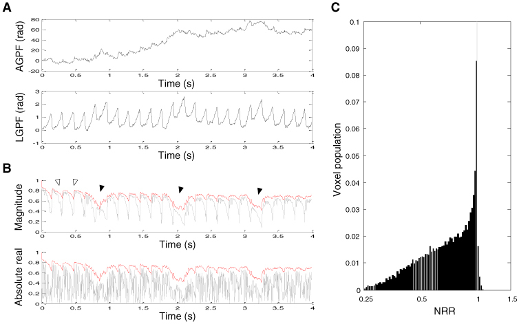
Effect of GPF correction. (A) Examples of axial and lateral global phase fluctuations found from axial and lateral data centered at the voxel a in Fig. 2B. (B) The cross-correlation of GPF-corrected images. Amplitudes of cardiac motion-oriented dips were remarkably reduced (empty arrows), whereas large respiratory motion-oriented dips remained (filled arrows). The gray line shows the cross-correlation of raw data. (C) Normalized population of the noise reduction ratio.

3.4 Correction of non-origin-centered global phase fluctuation

Although the GPF correction reduced noise in most voxels, some voxels were not affected by the correction because their complex-valued OCT signal rotated not around the origin but around some other point. This non-origin center of rotation might be attributed to the heterogeneous dynamics of particles within the voxel. If some particles remained stable while other particles moved within a single voxel, the OCT signal, which results from the interference of waves reflected from every particle, would rotate around a non-origin point. We examined the processing that finds the center of rotation (COR) for each voxel, subtracts the COR from the data, compensates for GPFs, and then restores the COR.

A COR was determined as a point in the complex plane where the deviation in the distances between the point and given data points was minimized. The distance between a point (A + iB) and the given signal at j-th time step (a_j + ib_j) is $D_j={(A-a_j)}^2+{(B-b_j)}^2$, and the deviation in this distance is

$$\begin{array}{l}{\sigma }_D^2=〈D_j^2〉-{\overline{D}}^2\\ =\frac{1}{N}{{\displaystyle \sum \left[{(A-a_j)}^2+{(B-b_j)}^2\right]}}^2-{\left[\frac{1}{N}{\displaystyle \sum \left\{{(A-a_j)}^2+{(B-b_j)}^2\right\}}\right]}^2\end{array}$$ (6)

where <> means averaging over time, and thus $〈D_j^2〉$ is the mean of squared distances. We derived solutions of A and B where the deviation is minimal:

$$\left[\begin{array}{cc}{\sigma }_a^2& 〈(a_j-\overline{a})b_j〉\\ 〈(b_j-\overline{b})a_j〉& {\sigma }_b^2\end{array}\right]\left[\begin{array}{c}A\\ B\end{array}\right]=\frac{1}{2}\left[\begin{array}{c}〈a_j^3〉-\overline{a}〈a_j^2〉+〈(a_j-\overline{a})b_j^2〉\\ 〈b_j^3〉-\overline{b}〈b_j^2〉+〈(b_j-\overline{b})a_j^2〉\end{array}\right]$$ (7)

where $\overline{a}$and $\overline{b}$are means of the real (a_j) and imaginary (b_j) parts of data points, respectively; and σ_a and σ_b are standard deviations of a_j and b_j, respectively.

An example of a non-origin COR is presented in Fig. 5A , where phase fluctuations rotating around the non-origin COR were effectively corrected. When this non-origin-centered GPF (NGPF) correction was applied to each voxel independently, 97.0% of the voxels showed a decrease in noise, which was 1.5% larger than that yielded by the GPF correction in the previous section. This result suggests that the noise of >480 voxels were reduced only by the non-origin-centered GPF correction. Time courses of the non-origin corrected AGPF, LGPF and cross-correlation were very similar to those of origin-centered GPF correction.

Fig. 5.

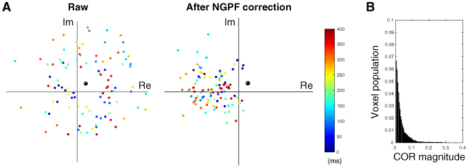
(A) An example of a non-origin center of rotation. Color dots display data points for complex-valued OCT signals for the first 400 ms (100 time points). The black circle indicates the center of rotation obtained by Eq. (7). (B) Normalized voxel population of the magnitude of the center of rotation. Nine percent of the voxels showed non-origin CORs whose magnitude was larger than 5% of the mean signal magnitude.

3.5 Optimization of algorithms

As described in the previous sections, respiratory motions mainly caused sub-pixel BISs, while cardiac motions caused GPFs. Although BISs and GPFs are coupled to one another, the BIS correction was more effective in reducing the amplitude of respiration-oriented dips in the cross-correlation, whereas the GPF correction was effective in cardiac motion-oriented decorrelation. One may consider several combinations of these processing steps to compensate for both types of motion artifacts. This study examined five combinations, as listed in Table 1 . In some combinations, the GPF correction was repeated in the order of axial, lateral, axial, lateral, axial directions, because we found that such repetition further, slightly removes GPFs.

Table 1. Combinations of BIS and GPF corrections.

C1	C2	C3	C4	C5
BIS	GPF (AL)	GPF (ALALA)	NGPF (ALALA)	GPF (ALALA)
GPF (AL)	BIS	BIS	BIS	BIS
	GPF (AL)	GPF (ALALA)	NGPF (ALALA)	GPF (ALALA)
				NGPF (ALALA)

GPF (AL): GPF correction for axial direction and then for lateral direction; GPF (ALALA): Repeating GPF corrections in the order of axial, lateral, axial, lateral, axial directions; NGPF: Non-origin-centered GPF correction.

As can be seen in Fig. 6A , each combination resulted in a different performance in terms of decorrelation suppression. C2 resulted in a better performance than C1, especially when cardiac and respiratory motions overlapped. This result suggests that it is helpful to correct GPFs prior to the BIS correction. C3 exhibited a slightly better performance than C2. Although the overall performance of C4 was similar to that of C3, C4 suppressed decorrelation more especially when the animal made respiratory motions. Finally, C5 resulted in a better performance than the other combinations. Taking into account that the increase in the number of repetitions did not lead to a large enhancement (from C2 to C3), the better performance of C5 with respect to that of C3 suggests that the NGPF correction in the last step worked additionally even after the GPF correction was sufficiently repeated. The NGPF correction resulted in significantly higher mean cross-correlation than the other combinations (Fig. 6B). In particular, the NGPF correction was effective in reducing noise at the surface (Fig. 6C). As a result, the phase fluctuations observed in Fig. 2B, for example, were dramatically reduced (Fig. 6D). The mean phase noise was reduced to 37%, and the phase noise decreased to less than 1% of its raw noise in more than 8% of the voxels (~2500 voxels).

Fig. 6.

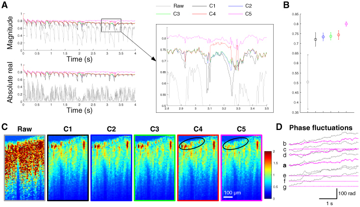
Performance of various combinations. (A) Cross-correlations of images for each combination. (B) The mean cross-correlation of the later two seconds. (C) Noise maps where each combination was applied. C5 was particularly effective in reducing noise at the surface (black circles), resulting in its higher cross-correlation than the other combinations. (D) The effect of C5 on fluctuations in the phase of the OCT signal from the voxels a-g in Fig. 2B.

The performance of the different combinations was validated across five animals. Similar relative performance was also observed in data from the other four animals (Fig. 7A ). Statistically, C5 resulted in significantly higher cross-correlation than C4 (Fig. 7B).

Fig. 7.

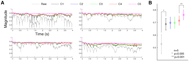
Performance of various combinations across animals. (A) The magnitude of cross-correlations in the data from four other animals. (B) The mean cross-correlation of the later two seconds across five animals. The error bar indicates the standard deviation of the mean cross-correlation across animals.

4. Discussion

The results of this study show that our algorithm was effective in suppressing decorrelation caused by cardiac and respiratory motions of the animal. Cardiac motions mainly caused GPFs, while respiratory motions caused BISs. Subsequent application of the GPF, BIS, GPF and NGPF corrections, the best combination among the various possibilities, significantly reduced the decorrelation, thus maintaining a high average image correlation of 0.76 ± 0.04 even after three seconds measured from five animals (Fig. 7B). In addition, the combination remarkably stabilized the phase of the OCT signal (Fig. 6D).

4.1 Choice of the reference frame

The choice of reference frame affected the performance of motion correction processing. This study chose the reference frame where cardiac and respiratory motions were most minimized. When we chose a reference frame from the middle of the cardiac/respiratory motions, the cross-correlation of raw data was lower and noisier. The mean cross-correlation magnitude of raw data decreased to 0.25 from 0.60. Also, the performance of motion correction was worse than that presented in this paper. The mean cross-correlation magnitude of the motion-corrected data was lower, 0.76 as opposed to 0.79.

Although we chose the first frame as the reference to better show decorrelation in time, it would be better during practical processing to choose a frame from the middle of the total acquisition time. This would lead to smaller noise because the performance of BIS and GPF correction is degraded as the time gap between the two frames increases. We used an algorithm to automatically find an optimized reference frame: every frame during one cycle of the cardiac motion in the middle of the acquisition time was tested to find the one producing the highest mean cross-correlation of raw data.

4.2 The number of upsampling

We upsampled images in the BIS correction to find sub-pixel shifts. This upsampling, however, requires a large amount of computation, thus making the BIS correction take much longer time than the GPF correction. Further, the computational load increases by the fourth power of the amount of upsampling. We tested various upsampling numbers from 2 to 8 and chose 4 because GPFs, which are partially coupled to sub-pixel BISs, were additionally corrected.

As an alternative means of compensating for sub-pixel shifts without the large computational load, we tested a Fourier transform-based method. First, we upsampled the cross-correlation for various pixel shifts (Eq. (2), rather than upsampling every image. From the upsampled shift-correlation relation, we found the sub-pixel shift maximizing the cross-correlation. Then, we compensated sub-pixel shifts with the Fourier transform.

$$R(z+\Delta z,x+\Delta x,t)=F^{-1}\left[\tilde{R}(k_z,k_x,t)e^{i{k}_z(z-\Delta z)+i{k}_x(x-\Delta x)}\right]$$ (8)

where $\tilde{R}(k_z,k_x,t)$ is the Fourier-transformed OCT signal and F⁻¹[ ] means the inverse Fourier transform. The computational load of this alternative method was much lower than that of the method based on explicit upsampling of every image (~1/100 smaller computation time); however, the performance was significantly lower, 0.768 ± 0.025 as opposed to 0.800 ± 0.018, in terms of the mean magnitude of cross-correlation.

4.3 Coupling between image shifts and global phase fluctuations

As described in the Results section, respiratory motions mainly caused BISs and cardiac motions caused GPFs. This relationship may not always be correct, however, as cardiac motions also can cause image shifts when they are so large as to cause supra-pixel movements of the brain. Therefore, it is more reasonable to understand that the BIS correction is more effective in compensating for motions larger than the pixel width, while the GPF correction is more effective in compensating for sub-pixel motions. Of course, the BIS correction could also suppress sub-pixel motion-oriented decorrelation if the amount of upsampling is sufficiently large. We confirmed that the amplitude of cardiac motion-oriented decorrelation (Fig. 3B) was further reduced when the BIS correction was applied with 16-fold image upsampling. This result implies that BISs and GPFs are coupled with one another, at least partially. Of course, the 16-fold upsampling required too much computational load to be of general utility.

4.4 Motion correction with a mask

As can be seen in the noise map (Fig. 6C), noise from vessels were much larger than those from stable tissue. Furthermore, when we looked at time courses of phase signals from vessels, the noise was too irregular to be related to global fluctuations. Those irregular noises might be attributed to movements of red blood cells. These movements (1-10 mm/s) are so fast with respect to our spatiotemporal resolution (3.5-7 μm and 4 ms) that OCT signals from vessel voxels may be totally uncorrelated after 1-2 time steps. As a result of this large decorrelation the complex-valued OCT signal appeared to be moving stochastically in the complex plane. Therefore, this irregular noise from vessel voxels might contaminate the cross-correlation in both BIS and GPF corrections (Eq. (2) and 3).

Another source of contamination was noise from the region of air and deep tissue. Since the amplitude of the OCT signal from those regions was so small, data points for the OCT signal looked like a Gaussian distribution in the complex plane. For this reason, the phase of those regions was very unstable and irregularly varying, thus contaminating the cross-correlation.

In order to minimize these contaminations, we examined a method using a mask. First, we applied the C3 method to find a relatively accurate noise map, and built a mask based on both noise and intensity maps. The mask had a value ranging from 0 to 1 at each voxel depending on its noise and intensity. Then, we used the mask in calculating the cross-correlation (Eq. 2 and 3) during application of the C5 method to raw data. It resulted in slightly lower (2%) noise in the tissue area (at a depth of 150-600 μm from the cortical surface). Of course, the use of a mask doubled the computation time, which can be a drawback in a practical analysis.

4.5 Feasible applications

Our motion correction processing can be helpful not only in noise reduction but also in enhancement of vessel structure visualization. Since the angiogram has been widely used in revealing vessel structures from dynamic OCT imaging data [6], this study compared angiograms of raw data and motion-corrected data where the C5 method was used. The angiogram was obtained with the time derivative of the OCT signal.

$$A(z,x)=\sqrt{{〈{\left|\frac{d}{dt}R(z,x,t)\right|}^2〉}_t}$$ (9)

This angiogram differs from the noise map in that it is proportional to the mean displacement of the OCT signal during one time step in the complex plane, whereas the noise map is the radius of the OCT signal distribution for the total acquisition time. For example, when a unit-magnitude OCT signal rotates π/100 at each time step for 200 time steps, the angiogram intensity is π/100 whereas the noise map intensity is 1. Therefore, the angiogram may better represent blood flow-oriented decorrelation when overall phase noise is large, because such a large phase noise results in the OCT signal rotating more than 2π for a given time (Fig. 5A, for example).

As can be seen in Fig. 8A , cross-sections of vessels were much more clearly evident in the motion-corrected angiogram. In contrast, the noise map and angiogram of raw data did not show much difference from the intensity map. This is likely due to large GPFs. A large GPF causes the OCT signal to rotate more than 2π in the complex plane and, as discussed above, such rotations make the deviation of signal similar to its magnitude. The angiogram can also be contaminated by large GPFs such as these because they make the displacement of the OCT signal in the complex plane much larger than that due to blood flow-oriented decorrelation.

Fig. 8.

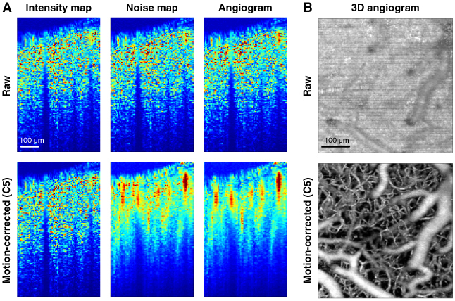
Effect of motion correction on the intensity map, noise map and angiogram. (A) The combination C5 in Table 1 was used for motion-corrected data. The brightness range for each map was automatically adjusted to the range from the mean of the lowest 1% to the mean of the highest 1%. (B) We also applied the C5 to 3D angiogram data. The maximum intensity projection of the 3D angiogram is shown as an en face image. Ten volumetric angiograms were averaged. A 10x objective was used for this angiogram.

Although we used as an example the cross-sectional angiogram obtained from the dynamic imaging data, general angiograms do not require such long-term dynamic imaging. Further, the proposed algorithms are intended for dynamic OCT imaging, not for structural imaging including angiograms. Nevertheless, it is worth showing how the proposed method works for 3D structural imaging (angiograms, for example). We performed another OCT scan for an angiogram, where B-scans were repeated two times for each cross-sectional plane (i.e., two time-points dynamic imaging) [6]. We used Eq. (9) to reveal vessel structures and performed maximum intensity projection through the z axis to obtain an en face image. As can be seen in Fig. 8B, we confirmed that the proposed method works very well not only for dynamic imaging but also for 3D angiography.

The motion correction algorithms presented in this paper would also be helpful in studies investigating time-varying physical quantities of tissue with phase-resolved optical methods. For example, the combination C5 is currently being used in one of our ongoing studies looking into depth-resolved hemodynamic responses of the cortex associated with functional activation. The combination C5 is effectively reducing cardiac and respiratory motion-oriented noise in our functional studies, thus enabling much clearer contrast in the hemodynamic responses.

5. Conclusion

This study demonstrated that an appropriate combination of BIS and GPF correction algorithms can efficiently suppress respiratory and cardiac motion-oriented noise in phase-resolved dynamic SD-OCT imaging of the rodent cerebral cortex. BISs and GPFs were observed to be produced mainly by respiratory and cardiac motions, respectively. We examined the cross-correlation maximization-based BIS correction, GPF correction, and non-origin-centered GPF correction. Several combinations of these corrections were tested to find the optimal one. The best combination enhanced image stability so that the cross-correlation remained 0.8 even after several seconds, while that of raw data was 0.5. It also significantly stabilized phase signals so that ~8% of the voxels showed noise reduction by two orders of magnitude. We have discussed several issues including choosing the reference frame, the coupling between BIS and GPF, and implementation of another method using a noise mask. As one of its possible applications, the optimized combination helped to reveal clearer vessel structures on an angiogram. Motion correction algorithms discussed in this paper would be helpful for general phase-resolved dynamic optical imaging of in vivo biological systems to reduce motion artifacts.