Iterated Prisoner’s Dilemma contains strategies that dominate any evolutionary opponent

Abstract

The two-player Iterated Prisoner’s Dilemma game is a model for both sentient and evolutionary behaviors, especially including the emergence of cooperation. It is generally assumed that there exists no simple ultimatum strategy whereby one player can enforce a unilateral claim to an unfair share of rewards. Here, we show that such strategies unexpectedly do exist. In particular, a player X who is witting of these strategies can (i) deterministically set her opponent Y’s score, independently of his strategy or response, or (ii) enforce an extortionate linear relation between her and his scores. Against such a player, an evolutionary player’s best response is to accede to the extortion. Only a player with a theory of mind about his opponent can do better, in which case Iterated Prisoner’s Dilemma is an Ultimatum Game.

Iterated 2 × 2 games, with Iterated Prisoner’s Dilemma (IPD) as the notable example, have long been touchstone models for elucidating both sentient human behaviors, such as cartel pricing, and Darwinian phenomena, such as the evolution of cooperation (1–6). Well-known popular treatments (7–9) have further established IPD as foundational lore in fields as diverse as political science and evolutionary biology. It would be surprising if any significant mathematical feature of IPD has remained undescribed, but that appears to be the case, as we show in this paper.

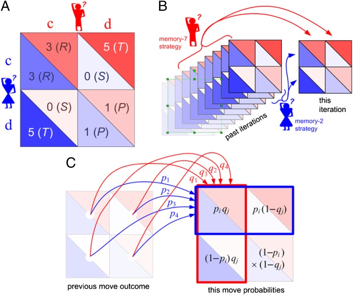
Fig. 1A shows the setup for a single play of Prisoner’s Dilemma (PD). If X and Y cooperate (c), then each earns a reward R. If one defects (d), the defector gets an even larger payment T, and the naive cooperator gets S, usually zero. However, if both defect, then both get a meager payment P. To be interesting, the game must satisfy two inequalities: T > R > P > S guarantees that the Nash equilibrium of the game is mutual defection, whereas makes mutual cooperation the globally best outcome. The “conventional values” occur most often in the literature. We derive most results in the general case, and indicate when there is a specialization to the conventional values.

Fig. 1.

(A) Single play of PD. Players X (blue) and Y (red) each choose to cooperate (c) or defect (d) with respective payoffs R, T, S, or P as shown (along with the most common numerical values). (B) IPD, where the same two players play arbitrarily many times; each has a strategy based on a finite memory of the previous plays. (C) Case of two memory-one players. Each player’s strategy is a vector of four probabilities (of cooperation), conditioned on the four outcomes of the previous move.

Fig. 1B shows an iterated IPD game consisting of multiple, successive plays by the same opponents. Opponents may now condition their play on their opponent’s strategy insofar as each can deduce it from the previous play. However, we give each player only a finite memory of previous play (10). One might have thought that a player with longer memory always has the advantage over a more forgetful player. In the game of bridge, for example, a player who remembers all of the cards played has the advantage over a player who remembers only the last trick; however, that is not the case when the same game (same allowed moves and same payoff matrices) is indefinitely repeated. In fact, it is easy to prove (Appendix A) that, for any strategy of the longer-memory player Y, shorter-memory X’s score is exactly the same as if Y had played a certain shorter-memory strategy (roughly, the marginalization of Y’s long-memory strategy: its average over states remembered by Y but not by X), disregarding any history in excess of that shared with X. This fact is important. We derive strategies for X assuming that both players have memory of only a single previous move, and the above theorem shows that this involves no loss of generality. Longer memory will not give Y any advantage.

Fig. 1C, then, shows the most general memory-one game. The four outcomes of the previous move are labeled for the respective outcomes , where c and d denote cooperation and defection. X’s strategy is , her probabilities for cooperating under each of the previous outcomes. Y’s strategy is analogously for outcomes seen from his perspective, that is, in the order of . The outcome of this play is determined by a product of probabilities, as shown in Fig. 1.

Methods and Results

Zero-Determinant Strategies.

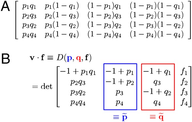
As is well understood (10), it is not necessary to simulate the play of strategies p against q move by move. Rather, p and q imply a Markov matrix whose stationary vector v, combined with the respective payoff matrices, yields an expected outcome for each player. (We discuss the possibility of nonstationary play later in the paper.) With rows and columns of the matrix in X’s order, the Markov transition matrix from one move to the next is shown in Fig. 2A.

Fig. 2.

(A) Markov matrix for the memory-one game shown in Fig. 1C. (B) The dot product of any vector f with the Markov matrix stationary vector v can be calculated as a determinant in which, notably, a column depends only on one player’s strategy.

Because M has a unit eigenvalue, the matrix is singular, with thus zero determinant. The stationary vector v of the Markov matrix, or any vector proportional to it, satisfies

Cramer’s rule, applied to the matrix , is

where is the adjugate matrix (also known as the classical adjoint or, as in high-school algebra, the “matrix of minors”). Eq. 2 implies that every row of is proportional to v. Choosing the fourth row, we see that the components of v are (up to a sign) the determinants of the 3 × 3 matrices formed from the first three columns of , leaving out each one of the four rows in turn. These determinants are unchanged if we add the first column of into the second and third columns.

The result of these manipulations is a formula for the dot product of an arbitrary four-vector f with the stationary vector v of the Markov matrix, , where D is the 4 × 4 determinant shown explicitly in Fig. 2B. This result follows from expanding the determinant by minors on its fourth column and noting that the 3 × 3 determinants multiplying each are just the ones described above. What is noteworthy about this formula for is that it is a determinant whose second column,

is solely under the control of X; whose third column,

is solely under the control of Y; and whose fourth column is simply f.

X’s payoff matrix is , whereas Y’s is . In the stationary state, their respective scores are then

where 1 is the vector with all components 1. The denominators are needed because v has not previously been normalized to have its components sum to 1 (as required for a stationary probability vector).

Because the scores s in Eq. 5 depend linearly on their corresponding payoff matrices S, the same is true for any linear combination of scores, giving

It is Eq. 6 that now allows much mischief, because both X and Y have the possibility of choosing unilateral strategies that will make the determinant in the numerator vanish. That is, if X chooses a strategy that satisfies , or if Y chooses a strategy with , then the determinant vanishes and a linear relation between the two scores,

will be enforced. We call these zero-determinant (ZD) strategies. We are not aware of any previous recognition of these strategies in the literature; they exist algebraically not only in IPD but in all iterated 2 × 2 games. However, not all ZD strategies are feasible, with probabilities p all in the range . Whether they are feasible in any particular instance depends on the particulars of the application, as we now see.

X Unilaterally Sets Y’s Score.

One specialization of ZD strategies allows X to unilaterally set Y’s score. From the above, X need only play a fixed strategy satisfying (i.e., set in Eq. 7), four equations that we can solve for and in terms of and , that is, eliminating the nuisance parameters and . The result, for general (not necessarily a PD game), is

With this substitution, Y’s score (Eq. 5) becomes

All PD games satisfy . By inspection, Eq. 8 then has feasible solutions whenever is close to (but ≤) 1 and is close to (but ≥) 0. In that case, is close to (but ≤) 1 and is close to (but ≥) zero. Now also by inspection of Eq. 9, a weighted average of P and R with weights and , we see that all scores (and no others) can be forced by X. That is, X can set Y’s score to any value in the range from the mutual noncooperation score to the mutual cooperation score.

What is surprising is not that Y can, with X’s connivance, achieve scores in this range, but that X can force any particular score by a fixed strategy p, independent of Y’s strategy q. In other words, there is no need for X to react to Y, except on a timescale of her own choosing. A consequence is that X can simulate or “spoof” any desired fitness landscape for Y that she wants, thereby guiding his evolutionary path. For example, X might condition Y’s score on some arbitrary property of his last 1,000 moves, and thus present him with a simulated fitness landscape that rewards that arbitrary property. (We discuss the issue of timescales further, below.)

X Tries to Set Her Own Score.

What if X tries to set her own score? The analogous calculation with yields

This strategy has only one feasible point, the singular strategy , “always cooperate or never cooperate.” Thus, X cannot unilaterally set her own score in IPD.

X Demands and Gets an Extortionate Share.

Next, what if X attempts to enforce an extortionate share of payoffs larger than the mutual noncooperation value P? She can do this by choosing

where is the extortion factor. Solving these four equations for the p’s gives

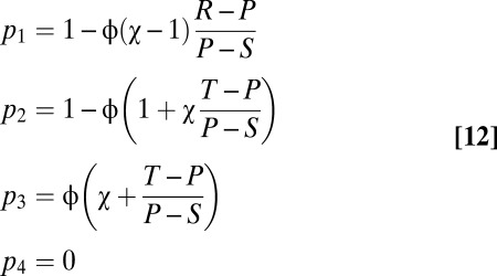Evidently, feasible strategies exist for any and sufficiently small . It is easy to check that the allowed range of is

Under the extortionate strategy, X’s score depends on Y’s strategy q, and both are maximized when Y fully cooperates, with . If Y decides (or evolves) to maximize his score by cooperating fully, then X’s score under this strategy is

The coefficients in the numerator and denominator are all positive as a consequence of . The case is formally allowed, but produces only the singular strategy mentioned above.

The above discussion can be made more concrete by specializing to the conventional IPD values ; then, Eq. 12 becomes

a solution that is both feasible and extortionate for . X’s and Y’s best respective scores are

With , X’s score is always greater than the mutual cooperation value of 3, and Y’s is always less. X’s limiting score as is 13/3. However, in that limit, Y’s score is always 1, so there is no incentive for him to cooperate. X’s greed is thus limited by the necessity of providing some incentive to Y. The value of is irrelevant, except that singular cases (where strategies result in infinitely long “duels”) are more likely at its extreme values. By way of concreteness, the strategy for X that enforces an extortion factor 3 and sets at its midpoint value is , with best scores about and .

In the special case , implying fairness, and (one of its limit values), Eq. 15 reduces to the strategy , which is the well-known tit-for-tat (TFT) strategy (7). Knowing only TFT among ZD strategies, one might have thought that strategies where X links her score deterministically to Y must always be symmetric, hence fair, with X and Y rewarded equally. The existence of the general ZD strategy shows this not to be the case.

Extortionate Strategy Against an Evolutionary Player.

We can say, loosely, that Y is an evolutionary player if he adjusts his strategy q according to some optimization scheme designed to maximize his score , but does not otherwise explicitly consider X’s score or her own strategy. In the alternative case that Y imputes to X an independent strategy, and the ability to alter it in response to his actions, we can say that Y has a theory of mind about X (11–13).

Against X’s fixed extortionate ZD strategy, a particularly simple evolutionary strategy for Y, close to if not exactly Darwinian, is for him to make successive small adjustments in q and thus climb the gradient in . [We note that true Darwinian evolution of a trait with multiple loci is, in a population, not strictly “evolutionary” in our loose sense (14)].

Because Y may start out with a fully noncooperative strategy , it is in X’s interest that her extortionate strategy yield a positive gradient for Y’s cooperation at this value of q. That gradient is readily calculated as

The fourth component is positive for the conventional values , but we see that it can become negative as P approaches R, because we have . With the conventional values, however, evolution away from the origin yields positive gradients for the other three components.

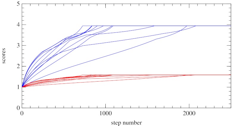
We have not proved analytically that there exist in all cases evolutionary paths for Y that lead to the maximum possible scores (Eq. 16) and that have positive directional derivatives everywhere along them. However, this assertion seems likely from numerical evidence, at least for the conventional values. Fig. 3 shows a typical numerical experiment in which X plays an extortionate strategy (here, , with maximum scores and ), and Y takes small steps that locally increase his score. Y has no unique gradient direction because the mapping from the score gradient (a covariant vector) to the step direction (a contravariant vector) involves an arbitrary metric, signifying how easily Y can evolve in each direction. Fig. 3 shows 10 arbitrary choices for this metric. In no case does Y’s evolution get hung up at a local maximum. That is, all of the evolutions shown (and all of a much larger number tried) reach the value of Eq. 14.

Fig. 3.

Evolution of X’s score (blue) and Y’s score (red) in 10 instances. X plays a fixed extortionate strategy with extortion factor . Y evolves by making small steps in a gradient direction that increases his score. The 10 instances show different choices for the weights that Y assigns to different components of the gradient, i.e., how easily he can evolve along each. In all cases, X achieves her maximum possible (extortionate) score.

Discussion

We have several times alluded to issues of timescale. The ZD strategies are derived mathematically under the assumption that the players’ expected scores are generated by a Markov stationary state defined by their respective strategies p and q. However, we have also suggested situations in which X may vary her ZD strategy so as to spoof Y with a fictitious fitness landscape. The question also arises whether Y can somehow vary his strategy on timescales faster than that for Markov equilibrium to be established. Perhaps by playing “inside the equilibration timescale” he can evade the linear constraint on scores (Eq. 7) imposed by X.

Interestingly, it is easy to prove that this latter situation cannot occur (Appendix B). If X plays a constant ZD strategy, then any strategy of Y’s, rapidly varying or not, turns out to be equivalent (from X’s perspective) to a fixed strategy against which X’s imposition of a constraint is effective.

In the former situation, where it is X whose strategies are changing (e.g., among ZD strategies that set Y’s score), things are not as crisp. Because X must be basing her decisions on Y’s behavior, which only becomes evident with averaging over time, the possibility of a race condition between X’s and Y’s responses is present with or without Markov equilibration. This reason is sufficient for X to vary her strategy only slowly. If X chooses components of p in Eqs. 9 and 8 that are bounded away from the extreme values 0 and 1, then the Markov equilibration time will not be long and thus not a consideration. In short, a deliberate X still has the upper hand.

The extortionate ZD strategies have the peculiar property of sharply distinguishing between “sentient” players, who have a theory of mind about their opponents, and “evolutionary” players, who may be arbitrarily good at exploring a fitness landscape (either locally or globally), but who have no theory of mind. The distinction does not depend on the details of any particular theory of mind, but only on Y’s ability to impute to X an ability to alter her strategy.

If X alone is witting of ZD strategies, then IPD reduces to one of two cases, depending on whether Y has a theory of mind. If Y has a theory of mind, then IPD is simply an ultimatum game (15, 16), where X proposes an unfair division and Y can either accept or reject the proposal. If he does not (or if, equivalently, X has fixed her strategy and then gone to lunch), then the game is dilemma-free for Y. He can maximize his own score only by giving X even more; there is no benefit to him in defecting.

If X and Y are both witting of ZD, then they may choose to negotiate to each set the other’s score to the maximum cooperative value. Unlike naive PD, there is no advantage in defection, because neither can affect his or her own score and each can punish any irrational defection by the other. Nor is this equivalent to the classical TFT strategy (7), which produces indeterminate scores if played by both players.

To summarize, player X, witting of ZD strategies, sees IPD as a very different game from how it is conventionally viewed. She chooses an extortion factor , say 3, and commences play. Now, if she thinks that Y has no theory of mind about her (13) (e.g., he is an evolutionary player), then she should go to lunch leaving her fixed strategy mindlessly in place. Y’s evolution will bestow a disproportionate reward on her. However, if she imputes to Y a theory of mind about herself, then she should remain engaged and watch for evidence of Y’s refusing the ultimatum (e.g., lack of evolution favorable to both). If she finds such evidence, then her options are those of the ultimatum game (16). For example, she may reduce the value of , perhaps to its “fair” value of 1.

Now consider Y’s perspective, if he has a theory of mind about X. His only alternative to accepting positive, but meager, rewards is to refuse them, hurting both himself and X. He does this in the hope that X will eventually reduce her extortion factor. However, if she has gone to lunch, then his resistance is futile.

It is worth contemplating that, though an evolutionary player Y is so easily beaten within the confines of the IPD game, it is exactly evolution, on the hugely larger canvas of DNA-based life, that ultimately has produced X, the player with the mind.

Appendix A: Shortest-Memory Player Sets the Rules of the Game.

In iterated play of a fixed game, one might have thought that a player Y with longer memory of past outcomes has the advantage over a more forgetful player X. For example, one might have thought that player Y could devise an intricate strategy that uses X’s last 1,000 plays as input data in a decision algorithm, and that can then beat X’s strategy, conditioned on only the last one iteration. However, that is not the case when the same game (same allowed moves and same payoff matrices) is indefinitely repeated. In fact, for any strategy of the longer-memory player Y, X’s score is exactly the same as if Y had played a certain shorter-memory strategy (roughly, the marginalization of Y’s long-memory strategy), disregarding any history in excess of that shared with X.

Let X and Y be random variables with values x and y that are the players’ respective moves on a given iteration. Because their scores depend only on separately at each time, a sufficient statistic is the expectation of the joint probability of over past histories H (of course in their proportion seen). Let , where is the recent history shared by both X and Y, and is the older history seen only by Y. Then a straightforward calculation is,

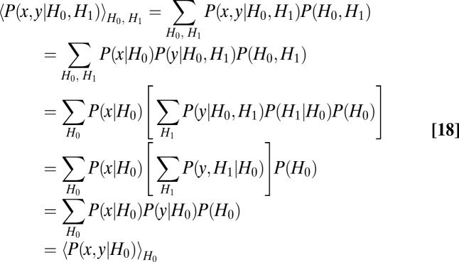Here, the first line makes explicit the expectation, and the second line expresses conditional independence.

Thus, the result is a game conditioned only on , where Y plays the marginalized strategy

Because this strategy depends on only, it is a short-memory strategy that produces exactly the same game results as Y’s original long-memory strategy.

Note that if Y actually wants to compute the short-memory strategy equivalent to his long-memory strategy, he has to play or simulate the game long enough to compute the above expectations over the histories that would have occurred for his long-memory strategy. Then, knowing these expectations, he can, if he wants, switch to the equivalent short-memory strategy.

To understand this result intuitively, we can view the game from the forgetful player X’s perspective: If X thinks that Y’s memory is the same as her own, she imputes to Y a vector of probabilities the same length as his own. Because the score for the play at time t depends only on expectations over the players’ conditionally independent moves at that time, Y’s use of a longer history, from X’s perspective, is merely a peculiar kind of random number generator whose use does not affect either player. So Y’s switching between a long- and short-memory strategy is completely undetectable (and irrelevant) to X.

The importance of this result is that the player with the shortest memory in effect sets the rules of the game. A player with a good memory-one strategy can force the game to be played, effectively, as memory-one. She cannot be undone by another player’s longer-memory strategy.

Appendix B: ZD Strategies Succeed Without Markov Equilibrium.

We here prove that Y cannot evade X’s ZD strategy by changing his own strategy on a short timescale—even arbitrarily on every move of the game. The point is that Y cannot usefully “keep the game out of Markov equilibrium” or play “inside the Markov equilibration time scale.”

For arbitrary p and q, the Markov matrix is as shown in Fig. 2A. We suppose that X is playing a ZD strategy with some fixed and write . The key point is that each row of is linear in exactly one component of q. Thus, the average of any number of different ’s satisfies

Now consider the result of N consecutive plays, where N is a large number. The game goes through N states , with . Comparing times i and , the game goes from state to state by a draw from the four probabilities , , where is the th component of (at time i). So the expected number of times that the game is in state is

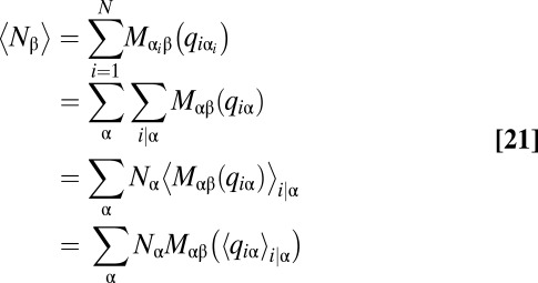Here the notation is to be read as “for values of i such that .”

Now taking the (ensemble) expectation of the right-hand side and defining probabilities

Eq. 21 becomes

This result shows that a distribution of states identical to those actually observed would be the stationary distribution of Y’s playing the fixed strategy . Because X’s ZD strategy is independent of any fixed strategy of Y’s, we have shown that, for large N, X’s strategy is not spoiled by Y’s move-to-move strategy changes.

That the proofs in Appendix A and Appendix B have a similar flavor is not coincidental; both exemplify situations where Y devises a supposedly intricate strategy that an oblivious X automatically marginalizes over.

References

- 1.Axelrod R, Hamilton WD. The evolution of cooperation. Science. 1981;211:1390–1396. doi: 10.1126/science.7466396. [DOI] [PubMed] [Google Scholar]
- 2.Roberts K. Cartel behavior and adverse selection. J Industr Econ. 1985;33:401–413. [Google Scholar]
- 3.Axelrod R, Dion D. The further evolution of cooperation. Science. 1988;242:1385–1390. doi: 10.1126/science.242.4884.1385. [DOI] [PubMed] [Google Scholar]
- 4.Nowak M, Sigmund K. A strategy of win-stay, lose-shift that outperforms tit-for-tat in the Prisoner’s Dilemma game. Nature. 1993;364:56–58. doi: 10.1038/364056a0. [DOI] [PubMed] [Google Scholar]
- 5.Nowak MA. Five rules for the evolution of cooperation. Science. 2006;314:1560–1563. doi: 10.1126/science.1133755. [DOI] [PMC free article] [PubMed] [Google Scholar]
- 6.Kendall G, Yao X, Chong SY. The Iterated Prisoners’ Dilemma 20 Years On. Singapore: World Scientific; 2007. [Google Scholar]
- 7.Axelrod R. The Evolution of Cooperation. New York: Basic Books; 1984. [Google Scholar]
- 8.Dawkins R. The Selfish Gene. New York: Oxford Univ Press; 1988. [Google Scholar]
- 9.Poundstone W. Prisoner’s Dilemma. New York: Doubleday; 1992. [Google Scholar]
- 10.Hauert Ch, Schuster HG. Effects of increasing the number of players and memory steps in the Iterated Prisoner’s Dilemma, a numerical approach. Proc Biol Sci. 1997;264:513–519. [Google Scholar]
- 11.Premack DG, Woodruff G. Does the chimpanzee have a theory of mind? Behav Brain Sci. 1978;1:515–526. [Google Scholar]
- 12.Saxe R, Baron-Cohen S, editors. Theory of Mind: A Special Issue of Social Neuroscience. London: Psychology Press; 2007. [Google Scholar]
- 13.Lurz RW. Mindreading Animals: The Debate over What Animals Know about Other Minds. Cambridge, MA: MIT Press; 2011. [Google Scholar]
- 14.Ewens WJ. An interpretation and proof of the fundamental theorem of natural selection. Theor Popul Biol. 1989;36:167–180. doi: 10.1016/0040-5809(89)90028-2. [DOI] [PubMed] [Google Scholar]
- 15.Güth W, Schmittberger R, Schwarze B. An experimental analysis of ultimatum bargaining. J Econ Behav Organ. 1982;3:367–388. [Google Scholar]
- 16.Nowak MA, Page KM, Sigmund K. Fairness versus reason in the ultimatum game. Science. 2000;289:1773–1775. doi: 10.1126/science.289.5485.1773. [DOI] [PubMed] [Google Scholar]