An Adaptive Window-setting Scheme for Segmentation of Bladder Tumor Surface via MR Cystography

Abstract

This paper proposes an adaptive window-setting scheme for non-invasive detection and segmentation of bladder tumor surface in T₁-weighted magnetic resonance (MR) images. The inner border of the bladder wall is firstly covered by a group of ball-shaped detecting windows with different radii. By extracting the candidate tumor windows and excluding the false positive (FP) candidates, the entire bladder tumor surface is detected and segmented by the remaining windows. Different from previous bladder tumor detection methods which are mostly focusing on the existence of a tumor, this paper emphasizes segmenting the entire tumor surface in addition to detecting the presence of the tumor. The presented scheme was validated by 10 clinical T₁-weighted MR image datasets (5 volunteers and 5 patients). The bladder tumor surfaces and the normal bladder wall inner borders in the ten datasets were covered by 223 and 10491 windows, respectively. Such large number of the detecting windows makes the validation statistically meaningful. In the FP reduction step, the best feature combination was obtained by using receiver operating characteristics or ROC analysis. The validation results demonstrated the potential of this presented scheme in segmenting the entire tumor surface with high sensitivity and low FP rate. This work inherits our previous results of automatic segmentation of the bladder wall and will be an important element in our MR-based virtual cystoscopy or MR cystography system.

I. Introduction

With the progress of medical imaging and computer technologies, more research efforts have been devoting to develop methods for task-specific imaging and computer aided detection and diagnosis (CAD). These research efforts have resulted in some efficient ways for detecting organ-specific abnormalities in a non-invasive or minimal invasive manner with some quantitative capability. The detection and classification of lung nodules [1] and colon polyps [2, 3] are two examples. Recently, the detection of bladder abnormality and classification of bladder tumor invasion depth [4, 5] have attracted more attention.

The statistics have shown that the chance of a man suffering from bladder cancer is about 1 in 27 while for women it is about 1 in 85. According to the survey of American Cancer Society, the bladder cancer becomes the fifth leading cause of cancer deaths in the United States due to its rapid increase (as high as 36% within a decade) [6-10]. The 5-year relative survival rate (the 5-year survival rate refers to the percentage of patients who live at least 5 years after their cancer is found and the 5-year relative survival rate assumes that patients will die of other causes as well.) of patients whose cancer is found in the third or fourth stage is below 50% [11]. In addition, the bladder tumor is reported to have high recurrence rate after resection (as high as 80%) [7]. Therefore, early detection and reexamination in the recovery stage of the bladder abnormalities via non-invasive methods are crucial for treatment of bladder carcinoma.

Fiberoptic cystoscopy which can accurately evaluate the bladder abnormalities is now the most popular diagnosis method. This method is performed, when the patient is placed in a lithotomy position, by inserting an endoscope through the urethra into the bladder. It was reported with a sensitivity of approximately 87% and specificity of around 95% [7, 12]. However, it is invasive, expensive, and time consuming, bringing great pain to the patients and increasing the risk of urinary tract infection and bleeding [13-15].

Nowadays, the development of medical imaging technologies has provided potential alternatives to the fiberoptic cystoscopy, such as virtual cystoscopy (VCys). The computed tomography (CT) and magnetic resonance imaging (MRI) are the mostly used imaging modalities for VCys [16, 17]. Preliminary results showed that there is no statistically significant difference between MR and CT cystography for detecting tumors by experts (sensitivity of 88.9% for tumors less than 10 mm and 100% for tumors equal or greater than 10 mm) [18-20]. The CT image can provide contrast for pathological changes of the mucous membrane (not less than 2 mm) [21]. Although the above computerized VCys results cannot be used as the final decision, they provide valuable reference assisting the doctor for clinical assessment. In both CT and MR bladder images, it is expected that the morphology and texture features extracted from bladder tumor and normal bladder wall are distinguishable from each other. Comparing with the CT imaging modality, the MRI is preferred because it is non-invasive, without ionization radiation, and provides better soft tissue contrast with structural, functional and pathological information. Therefore, MRI makes it possible to perform more delicate analyses, such as digging out the tumor region and staging the tumor growth. For example, the T₁-weighted MR images provide better contrast for the bladder wall which is crucial for bladder abnormality detection [19]. According to previous reports, features on the bladder wall, such as curvedness (CV), shape index (SI), and the bladder wall thickness [14, 15, 22-24] are useful for detecting bladder tumors. For example, the sensitivity of bladder tumor detection by using the wall thickness as the individual parameter reached 83%-89% [15]. Wu, et al., [5] found some texture features from T₂-weighted MR images are able to distinguish bladder tumor from normal bladder wall. They also showed some results of staging the tumor growth based on the detection results. The bladder and detected abnormalities are displayed to the experts by using computer graphic techniques, which have two basic components of (1) constructing a three-dimensional (3D) bladder model and (2) displaying some features of a possible tumor on the 3D model [23-25]. All the techniques above only indicate the existence of the bladder tumors instead of giving the tumor region clearly.

Comparing with the above related studies which only detect the existence of bladder tumors, this work emphasizes the delineation of the entire tumor surface by an automatic fashion. In other words, the former focuses on the detection of the presence of a tumor while the latter emphasizes on the segmentation of the extent of a tumor. Our preliminary research [26] proved that by using the detected portion of the tumor surface as initial, we can trace inward and dig out the tumor portion buried inside the bladder wall. Digging out the whole tumor surface is valuable for measuring the tumor size, tumor stage and invasion level. The associated image processing techniques can capture and render tumor features which are unobservable to the experts on the images. So far, no reports have given satisfied results for tumor surface segmentation. Our previous study [26] only roughly outlined a portion of the tumor surface by using geometry features. This paper introduces a method which focuses on the segmentation of the entire tumor surface. By combining the work in this paper and in [26], it is possible to dig out the integrated tumor region with a portion protruding from the bladder wall and the other portion being inside the wall. The method is based on an adaptive window-setting scheme, uses T₁-weighted MR images, and assumes that the geometry, texture, wall thickness and regional statistics extracted from the bladder tumor and normal bladder wall are distinguishable.

The remainder of this paper is organized as follows. Section II illustrates the flowchart of the proposed tumor surface segmentation. Section III briefly reviews our previous bladder wall segmentation strategy [27]. Section IV describes how the window radius is determined and how the windows are arranged on the segmented inner border of the bladder wall. The candidate window selection and false positive (FP) window reduction are introduced in section V. Section VI reports the results and presents some discussions, followed by conclusions in Section VII.

II. Overview

The flowchart of the tumor surface segmentation is shown in Fig. 1. First, the inner and outer borders of the bladder wall in a T₁-weighted MR image volume were segmented by using the coupled level set framework (Section III). Windows were aligned in such a way that their centers are on the segmented inner border of the bladder wall. The window radius was adaptive to the geometry condition of the inner border in order to guarantee each window contains no more than one structure (Section IV). The SI and weighted bladder wall thickness (WT) were extracted from each window. The candidate windows which are likely to include tumor image voxels were picked out by using predefined thresholds on the SI and WT. More features about the geometries, textures and regional statistics were extracted from the candidate windows and used to construct the feature spaces. The best-performed feature combination was obtained by receiver operating characteristics (ROC) analysis to reduce the FPs in the candidate windows. The final tumor windows were determined by applying the discriminant analysis in the feature space (Section V).

Fig. 1.

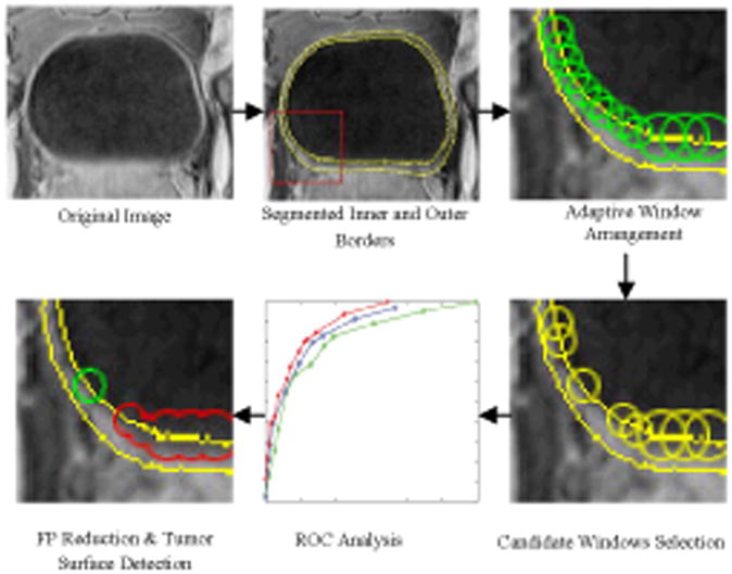
Pipeline of the bladder tumor surface segmentation by an adaptive window scheme.

III. Review of the Bladder Wall Segmentation

This section briefly reviews the coupled level set method for bladder wall segmentation. The coupled level set method was described in detail in our previous work [27]. The segmentation was automatically performed on the clinical MR images and the precision was proved by the radiologists. The level set functions used in the segmentation were also used in the following procedures.

The MR imaging procedure is non-invasive by using the urine as the endogenous contrast agent. As shown in Fig. 2, the T₁-weighted MR image provides better bladder wall contrast than the T₂-weighted MR image due to the decreased urine intensity. In addition, the partial volume (PV) effect in the T₁-weighted image goes from wall toward the lumen and is less visible, while in the T₂-weighted image it goes from lumen into the wall and can “swallow” small abnormal growth on the inner border. Therefore, the segmentation was performed on the T₁-weighted MR images [27-29]. Before segmentation, a linear interpolation procedure was performed, due to the different intra- and inter-slice resolutions. The intensity value of each interpolated voxel is the linear combination of its 6-connection neighborhood.

Fig. 2.

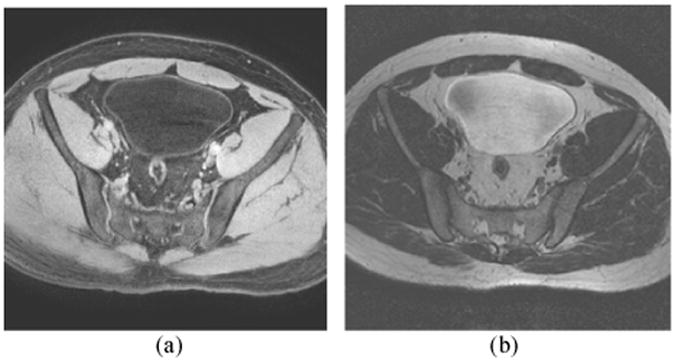
Typical bladder MR images. (a) T₁-weighted MR image. (b) T₂-weighted MR image. The bladder wall is more distinguishable in the T₁ image than in the T₂ image.

The level set method was first proposed by Osher and Sethian as a geometric deformable model to implicitly describe evolving surfaces (or a curve in 2D case) [30]. In [27], the work [30] was adapted for a coupled level set approach to segment the bladder wall borders automatically. The inner and outer borders were segmented simultaneously by using φ₁ and φ₂, where φ₁ and φ₂ are the inner level set function (ILSF) and outer level set function (OLSF), respectively. The inner and outer borders are represented by the zero level set surfaces (ZLSSs) of the ILSF and OLSF.

First, the ZLSS of the ILSF φ₁ was initialized as a ball shaped region inside the bladder lumen. The inner border of the bladder wall was segmented by a modified version from the original C-V model [31]. Then, φ₂ evolved several steps outward from the φ₁ to estimate the location of the outer border. Generally, the outer border of the bladder wall has similar shape as the inner border. The geometry property of φ₁ provides prior information for initializing and evolving φ₂. Since the intensity contrast between the bladder wall and the tissues outside the bladder wall is relatively poor and the intensity distribution of the surrounding tissues is complex, the geometry information from the ILSF is necessary for the outer border segmentation. After the inner and outer borders of the bladder wall were roughly estimated by the ZLSSs of φ₁ and φ₂, a regional adaptive clustering algorithm [27] was applied to further evolve the above two functions iteratively. The evolution stopped when a predefined energy is minimized. Fig. 3 shows an example of the segmentation result. The yellow curves are the segmented borders in this slice. More results from the coupled level set framework are reported in [27].

Fig. 3.

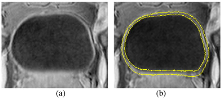
(a) A typical slice of the T₁-weighted MR image. (b) Segmentation result of the image in (a). The two yellow curves are the segmented inner and outer borders represented by ZLSSs of φ₁ and φ₂.

IV. Adaptive Window-setting Scheme

A. Window Design and Arrangement

Instead of performing voxel by voxel detection, detecting windows were designed, which were arranged throughout the segmented inner border. This idea is based on the ground truth that the bladder tumor emerges firstly on the mucosa layer (close to the inner border of the bladder wall), and then invades gradually inside the muscle layer. Therefore, the regions around the bladder wall inner border provide useful information for tumor detection. The centers of the detecting windows were aligned on the inner border. To make the window features invariant to rotation, the detecting windows are ball shaped. The windows overlapped to each other to guarantee the inner border is totally covered. The window size was determined by the ball radius which varies at different locations. The windows together constructed a band-shaped region around the inner border. The possible tumor surface were finally detected and also covered by a group of windows.

Fig. 4(a) shows an example of the window arrangement. Generally, the two adjacent windows overlap each other by putting one window's center on the other window's border. Fig. 4(b) takes the bladder wall thickness as an example to show how the features are extracted from the windows. The blue curves are the bladder wall borders. The shadow between the two curves represents the bladder wall/tumor region. The numbers are the OLSF values, and are also the distance from the voxels to the outer border. If a voxel is on the inner border, the corresponding number indicates the wall thickness at this voxel. The OLSF values were recorded in float. We converted them to integer for illustration purpose in Fig. 4(b). Suppose the upper and the lower windows lie on the bladder tumor (the protrusion) and normal bladder wall respectively, then the wall thicknesses at the window central voxels would be 6.0 and 5.0 respectively. The mean wall thicknesses would be 6.5 and 5.0, which were computed by averaging all numbers inside the windows. Therefore, the central voxel thickness and the mean thickness both have the potential of distinguishing these two windows.

Fig. 4.

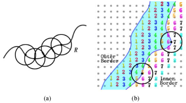
An example of the window arrangement and feature extraction. (a) The adjacent windows overlap each other. (b) Two windows on the inner border of the bladder wall with the numbers indicating the distance from each voxel to the outer border.

B. Window Radius Determination

All the features used for tumor candidate detection and FP reduction were captured from the windows, which are the basic elements for tumor surface segmentation. If a window is detected as a tumor window, then the region inside the window is considered as tumor region. Therefore, the window size should be properly set. We used “structure” to denote a continuous region on the bladder wall. One structure should include only one tissue type, and this guarantees the inner geometry/intensity property varies smoothly. The tumor and the bladder wall are different structures. Furthermore, the region including the same tissue but with prominent geometry variations also belongs to different structures. If a window including more than one structure, the window radius should be reduced. Fig. 5 shows an example that two structures are inside one window.

Fig. 5.

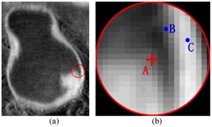
An example to show the different structures inside one window. (a) The original image. The red circle indicates the window border. (b) The enlarged image in the red circle in (a). The red cross A is the center of the window. B and C are two voxels.

The red cross A is at the window center, B and C are voxels within the same window. A is on the tumor while B and C are on the bladder wall. The gap between A and B/C is the bladder lumen. The current window radius should be reduced to exclude B and C as well as all other voxels on the bladder wall. Then, the features extracted from this window represent the bladder tumor, the same as the features from the window central voxel. On the other hand, even if voxels A, B and C are of the same tissue type, they also belong to different structures due to their discontinuous geometry properties, such as the intensity gradient. Therefore, the voxels B and C should be excluded from this window as well. Generally, the window radius would be set to include enough voxels from the same structure to guarantee the features are statistically reliable, while excluding as much as possible the unconcerned structure voxels. In other words, a bigger window would likely include unrelated structures inside, while a smaller window could be more vulnerable to the image noise. A simulative bladder tumor image and the adaptive window radius selection scheme are depicted in Fig. 6.

Fig. 6.

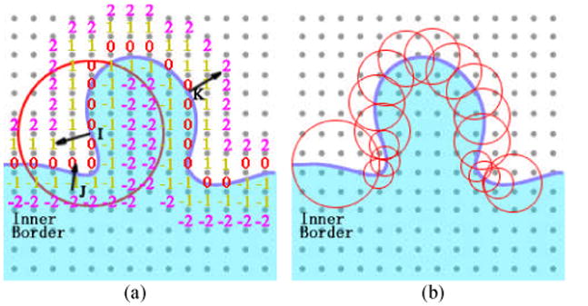
The distance function-based gradients used to distinguish different topological structures in the windows.

As shown in Fig. 6, the protrusion represents the emerging tumor. I, J, and K are three voxels on and inside the inner border. The red circle is the boundary of a 3D window on this slice. As mentioned above, the inner border of the bladder wall was obtained by the ILSF which has the form of distance function [27]. The numbers in Fig. 6(a) are the distance from an arbitrary voxel to the nearest voxel on the inner border. The black arrows indicate the gradient directions at the three voxels. A possible condition is shown by Fig. 6(a) that a window locates at the foot of a tumor. J is a voxel on the normal bladder wall and K lies on the other side of the tumor. Since J and I are on different tissues (wall and tumor) and I is the window center, then voxel J should be excluded from this window. In other words, the window shall represent the tumor surface that the voxel I belongs to. The voxel K should also be excluded from the window. If K is included, not only the tumor surface but also the bladder wall and the central part of the tumor would contribute to the window features. More specifically, as mentioned above, the bladder tumor emerges on the inner border and then invades toward the muscle layer. The texture features inside the tumor are considered to be different layer by layer. Suppose both I and K are inside one window, then delicate texture variation among layers would be diminished.

To distinguish the voxels belonging to different structures, the gradient of the distance function was used. As shown in Fig. 6(a), the gradient direction at J and K are distinctly different from that at voxel I. Suppose the angle between the gradient directions at center voxel I and another voxel J is angle(I,J), (0≤ angle (I,J) ≤π), with a predefined angle θ₀, a labeling function L(angle(I,J)) is obtained, which is

$$L\left(\mathit{\text{angle}}\left(I,J\right)\right)=\{\begin{array}{cc}1& \mathit{\text{angle}}\left(I,J\right)<{\theta }_0\\ 0& \mathit{\text{otherwise}}\end{array}.$$ (1)

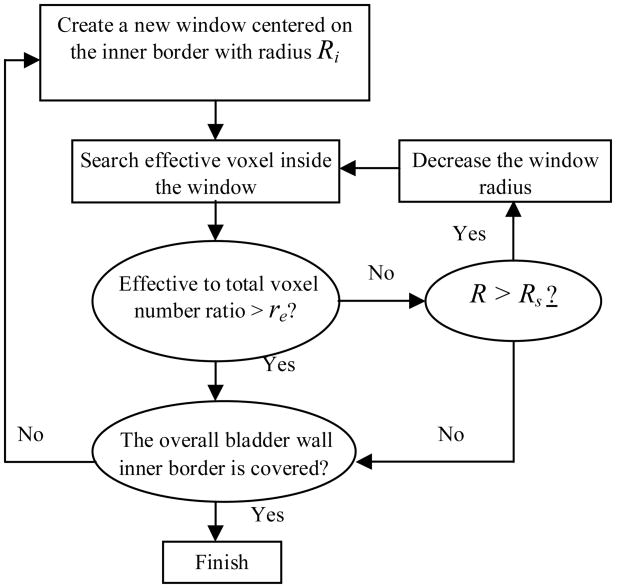
If L=1, then I and J are considered to be in the same structure, otherwise, J is excluded. Let the voxels with L=1 being the effective voxels. If the number of effective voxels is too small with respect to the total voxel number in one window (smaller than a predefined ratio r_e), it means the window is close to the boundary of two adjacent structures and a smaller window is needed. Fig. 6(b) gives an example to depict this concept. The windows cover the inner border one by one. The bigger windows are aligned on the smoother border sections such as the normal bladder wall, while the small windows are located on the region with mixed structures, such as the tumor foots. Since the windows overlap each other, the overlapped regions are considered as the tumor if it is covered by at least one tumor window. Fig. 7 illustrates the flowchart of the window radius determination procedure. The windows should cover the whole region of the bladder wall inner border. The procedure includes: (1) An initial and stop window radii were defined as R_i and R_s. (2) A new window was created on the inner border, and this window radius was set to be. R=R_i. (3) The labeling function L was renewed for all voxels inside the window. If the effective to total voxel ratio was smaller than the predefined r_e, then the window size was decreased by set R=R-2. (4) If the effective to total voxel ratio was bigger than the predefined r_e or the stop radius R_s was reached, then the window radius R was obtained. Otherwise, the operation went back to step (3). (5) Features were extracted from the window. (6) The operation went back to step (2). The center of the new window was set on the border of the current window. The above iteration procedure stopped until the windows cover the whole inner border.

Fig. 7.

Flowchart of the adaptive window assignment.

The values of θ₀ and r_e were selected by experiments. Both θ₀ and r_e work together to exclude as much as possible the unconcerned structures, and guarantee a window has a similar scale as the structure inside. Therefore, the window radii distribution depends on the θ₀ and r_e values. With the given θ₀ and r_e values, the R_i should be set larger than most of the window radii. More discussion on the values of θ₀, r_e, R_i and R_s will be given in Section VI.

V. Candidate Detection and False Positive Reduction

A. Tumor Candidate Detection

Previous work proved that bladder wall thickening is an evidence of existence of bladder tumor [14, 15, 21, 23, 24]. And it is widely accepted that the bladder tumor appears as protrusions on the inner border of the bladder wall. By assuming that a surface is defined by an iso-contour (the iso-intensity surface), the geometry-related features such as the gradient and the SI can be computed directly from the partial derivatives of the 3D image intensity functions (the image data) [32]. These features are good indicators of the protrusions on the inner border. We had used the SI for colon polyp detection [33] and obtained encouraging results. The partial derivatives of the 3D image are defined as:

$$\begin{array}{l}{o}_0\left(x\right)=c_0\left(1+\alpha \left|x\right|\right)e^{-\alpha \left|x\right|}\\ o_1\left(x\right)=-c_{1}x{\alpha }^2{e}^{-\alpha \left|x\right|}\\ o_2\left(x\right)=c_2\left(1-c_3\alpha \left|x\right|\right)e^{-\alpha \left|x\right|}\end{array}$$ (2)

where o₀, o₁, and o₂ are the smooth, first, and second derivative operators, respectively. The value of α controls the smoothing degree and should be specified in advance. We set α = 1.0 throughout our experimental work. The normalization coefficients c₀ to c₃ are determined by ${\int }_{-R}^R{o}_0\left(x\right)dx=1,{\int }_{-R}^{R}x{o}_1\left(x\right)dx=1,{\int }_{-R}^R{o}_2\left(x\right)dx=0\text{and}{\int }_{-R}^R\frac{x^2}{2}{o}_2\left(x\right)dx=1$.

In our case, the operating domain was inside the window. Given the image function I=I(x), the smoothed partial derivatives of I at voxel x=(x,y,z) are calculated by

$$\begin{array}{l}{I}_x=\left(o_1\left(x\right)o_0\left(y\right)o_0\left(z\right)\right)\ast I\left(\mathbf{\text{x}}\right)\\ I_{\mathit{\text{xx}}}=\left(o_2\left(x\right)o_0\left(y\right)o_0\left(z\right)\right)\ast I\left(\mathbf{\text{x}}\right)\\ I_{\mathit{\text{xy}}}=\left(o_1\left(x\right)o_1\left(y\right)o_0\left(z\right)\right)\ast I\left(\mathbf{\text{x}}\right).\end{array}$$ (3)

The principal curvatures at voxel x are represented by κ₁(x) and κ₂(x). The formulations of κ₁(x) and κ₂(x) can be found in [32], which are based on the operators in Eqs. (2) and (3). Furthermore, the SI is computed by using κ₁(x) and κ₂(x) according to

$$\mathit{\text{SI}}=0.5-\left(1/\pi \right)\text{arctan}\left({\kappa }_1+{\kappa }_2/{\kappa }_1-{\kappa }_2\right).$$ (4)

When the SI value is ranging from 0.0 to 1.0, the surface shape varies from cup, rub, saddle, ridge, to cap. Generally, the bladder tumor region is rut-shaped at the tumor foot and cap-shaped at the central part of tumor surface, with the SI value close to 0.0 and 1.0, respectively.

The bladder wall thickness was also obtained by using the windows. Let T be the thickness value at a voxel in the window, which is measured by the OLSF φ₂ as mentioned above. Therefore, we have T=φ₂(x) at voxel x. Within a window, a weighted thickness (WT) and normalized weighted thickness (NWT) were obtained by

$$\begin{array}{l}\mathit{\text{WT}}=\frac{{\int }_{\Omega }I\left(\mathbf{\text{X}}\right){\phi }_2\left(\mathbf{\text{X}}\right)L\left(\mathit{\text{angle}}\left(\mathbf{\text{X}},c\right)\right)d\mathbf{\text{X}}}{{\int }_{\Omega }I\left(\mathbf{\text{X}}\right)L\left(\mathit{\text{angle}}\left(\mathbf{\text{X}},c\right)\right)d\mathbf{\text{X}}}\\ \mathit{\text{NWT}}=\frac{\mathit{\text{WT}}}{\overline{\mathit{\text{WT}}}}.\end{array}$$ (5)

where Ω is the image domain inside the window. The labeling function L was defined in Eq. (1). $\overline{\mathit{\text{WT}}}=\mathit{\text{mean}}\left(\mathit{\text{WT}}\right)$ is the mean WT value of all windows of the current dataset. Since the bladder wall is thinner when the bladder is full of urine than empty, the WT value at the same place varies according to the bladder status. Therefore, the NWT of each data was used instead of the WT.

So far, two features – the SI and NWT have been computed from each window. Based on these two features, a group of predefined thresholds were used to pick out the candidate windows as listed in Table III. The windows with corresponding values between the maximum and minimum thresholds were selected as the candidate windows.

Table III. Threshold Values of the Operators for Candidates Detection.

	Operator	Value
SI	Lower Thresholds	0.00-0.05
	Higher Thresholds	0.95-1.00
NWT	Minimum value	1.10
	Maximum value	-

B. Volumetric Features for False Positive Reduction

As described above, a group of pre-defined thresholds of the SI and NWT features were used to select candidates in order to guarantee all the tumor windows are picked up. In consequence, the candidates may include FP windows. Various reasons, such as the extrusion of the prostate, may lead to the geometry changes of the bladder wall and produce the FP windows. Therefore, FP reduction is necessary. Additional features, especially texture information from the windows, which can reflect the differences between the FP windows and the true tumor windows, are needed. Comparing with the CT images, the MR images provide more delicate textural information for the soft tissue such as the bladder wall and the tumor. Furthermore, considering the fact that the tumor invades gradually from the mucosa layer toward the muscle layer, the feature variation among layers should be able to distinguish the tumor surface from the normal bladder wall inner border. Therefore, in addition to the SI and the NWT, other two groups of features were considered. One is the window statistics, and the other one is the layer-based features. These two groups of features were generated from three voxel-based raw features, which are the intensity value I, intensity gradient G_I and distance function gradient G_φ. Let w_i represent the ith candidate window, |w_i| be the number of voxels in the window, and f^j(j = 1,2,3) represent the I, G_I and G_φ together, where the gradient values G_I and G_φ were generated from the first order neighborhood, the G_φ was the gradient value of the ILSF φ₁(x), and the f^j of each voxel was computed in advance. Seven window statistics for each raw feature f^j in window w_i are computed as:

$$\begin{array}{l}\text{mean}\left(w_i,f^j\right)={\mu }_{\mathit{\text{ij}}}=\sum _{\mathbf{\text{x}}\in w_i}\frac{f^j\left(\mathbf{\text{x}}\right)}{\left|w_i\right|}\\ \text{var}\left(w_i,f^j\right)={\sigma }_{\mathit{\text{ij}}}^2=\frac{1}{\left|w_i\right|-1}\sum _{\mathbf{\text{x}}\in w_i}{\left(f^j\left(\mathbf{\text{x}}\right)-{\mu }_{\mathit{\text{ij}}}\right)}^2\\ \text{min}\left(w_i,f^j\right)=\underset{\mathbf{\text{x}}\in w_i}{\text{min}}\left\{f^j\left(\mathbf{\text{x}}\right)\right\}\\ \text{max}\left(w_i,f^j\right)=\underset{\mathbf{\text{x}}\in w_i}{\text{max}}\left\{f^j\left(\mathbf{\text{x}}\right)\right\}\\ \text{skew}\left(w_i,f^j\right)=\frac{1}{\left|w_i\right|}\sum _{\mathbf{\text{x}}\in w_i}{\left(\frac{f^j\left(\mathbf{\text{x}}\right)-{\mu }_{\mathit{\text{ij}}}}{{\sigma }_{\mathit{\text{ij}}}}\right)}^3\\ \text{kurt}\left(w_i,f^j\right)=\frac{1}{\left|w_i\right|}\sum _{\mathbf{\text{x}}\in w_i}{\left(\frac{f^j\left(\mathbf{\text{x}}\right)-{\mu }_{\mathit{\text{ij}}}}{{\sigma }_{\mathit{\text{ij}}}}\right)}^{4}3\\ \text{contrast}\left(w_i,f^j\right)=\frac{\text{min}\left(w_i,f^j\right)}{\text{max}\left(w_i,f^j\right)}.\end{array}$$ (6)

where μ_ij and σ_ij are the mean and standard deviation of f^j in w_i, min(w_i, f^j) and max(w_i, f^j) are the minimum and maximum f^j values in w_i. Other statistics were calculated by using μ_ij, σ_ij, min(w_i, f^j) and max(w_i, f^j) and |w_i|.

The layer-based features were computed by using the ILSF φ₁. While the OLSF φ₂ represents the bladder wall thickness, the φ₁ divides one window into several layers. As shown in Fig. 6(a), the layer with index l (an integer) includes voxel x, where l(x) −0.5≤φ₁(x) <l(x)+0.5. For example, l(x)=-1 includes those voxels x where −1.5≤φ₁(x) <−0.5, and l(x)=0 includes those voxels x where −0.5≤φ₁(x) <0.5. The layer-based features were computed by

$$\mathit{\text{dev}}\left(l,f^j\right)=o_1\left(l\left(\mathbf{\text{x}}\right)\right)\ast f^j\left(l\left(\mathbf{\text{x}}\right)\right).$$ (7)

where, the o₁ was defined in Eq. (2) as the first derivative operator. By using l(x) instead of x as the variable, Eq. (7) is 1D derivative, which reflects the feature variation among layers.

For each raw feature j, seven statistics plus one layer-based features were computed, which means totally 24 features were generated from the three raw features. Together with the SI and NWT, there are totally 26 features extracted from each window.

C. Segmentation of the Entire Tumor Surface

In this section, the description goes to the reduction of FPs and the use of the final windows to construct the tumor surface regions. As mentioned in the last section, 26 features from window i have been extracted and will be used to perform the discrimination. These features construct a 26D feature vector ${\mathbf{\text{F}}}_i=\left(F_i^1,F_i^2,F_i^3,\cdots F_i^{26}\right)$ .

The quadratic discriminant analysis (QDA) [34] was used to classify the windows as either true positive (TP) or FP. The windows were separated into two groups, the training group and the testing group. The tumor regions were labeled by experts in advance, i.e., each voxel was labeled as either normal bladder wall or tumor. The window type in the training group is the same as its central voxel. The candidate windows with the central voxel labeled “tumor” are the TP while the windows with the central voxel labeled “wall” are the FP. The mean and covariance matrices of the TP (μ_TP, Σ_TP) and FP (μ_FP, Σ_FP) samples in the training group were computed.

In the testing group, a feature vector F_i was extracted from window i. The quadratic discriminant function was applied to classify TPs and FPs and has the form of

$$g\left({\mathbf{\text{F}}}_i\right)=-{\left({\mathbf{\text{F}}}_i-{\mathbf{\mu }}_{\mathit{\text{TP}}}\right)}^T{\sum }_{\mathit{\text{TP}}}^{-1}\left({\mathbf{\text{F}}}_i-{\mathbf{\mu }}_{\mathit{\text{TP}}}\right)+{\left({\mathbf{\text{F}}}_i-{\mathbf{\mu }}_{\mathit{\text{FP}}}\right)}^T{\sum }_{\mathit{\text{FP}}}^{-1}\left({\mathbf{\text{F}}}_i-{\mathbf{\mu }}_{\mathit{\text{FP}}}\right).$$ (8)

The decision boundary is a hyperquadratic surface in the feature space where g(x)= t. The final decision is based on which side the feature vector is located in the feature space. The discriminant is given by

$$\text{window}i=\{\begin{array}{cc}\text{TP},& \text{if}g\left({\mathbf{\text{F}}}_i\right)\ge t\\ \text{FP},& \text{if}g\left({\mathbf{\text{F}}}_i\right)<t\end{array}$$ (9)

where t is a predefined constant.

It is noted that the datasets generated a large amount of detecting windows. Each dataset could result in far more than one feature vector. Furthermore, a tumor could be covered by several detecting windows. Therefore, a large amount of abnormal windows were generated for training from a relatively small number of patients' datasets.

VI. Results and Discussion

A. Data Acquisition

Ten T₁-weighted MR image datasets, five patients and five volunteers, were used to test the above presented segmentation method. All subjects were asked to empty the bladder and drink a cup of water about a half hour prior to the scanning so that the bladder was full of the urine when scanning started. The whole imaging procedure is noninvasive. The image data was acquired in DICOM format by using a clinic whole body 3.0T scanner. The original DICOM datasets were reformed to self-defined raw volumes with the subjects' private information being removed. Considering the anisotropic resolution of the images, a linear interpolation was performed. Then the coupled level set framework was applied to segment the inner and outer borders of the bladder wall automatically. The patients' datasets were inspected by experts, and the tumors were labeled manually in advance by the experts for comparison and evaluation purposes. Table I lists the scanning protocols, the repetition time and the echo time for acquiring the ten datasets.

Table I. Data Information and Image Acquisition Parameters.

Dataset	Scanning Protocol	TR (ms)	TE (ms)
1	3dffe-SPIR Clear	4.6666	2.2766
2	2500 Full Scan Clear	4.6747	2.2818
3	3d 25 Min Clear	4.6679	2.2756
4	MPR COR	4.6679	2.2756
5	Thri Pelpre Sense	4.3896	2.1181
6	bSPIR 3nex Clear	4.6750	2.2818
7	SPIR 2nex Clear	4.6747	2.2818
8	3DFFE-SPIR Clear	4.6747	2.2818
9	Thrive Pre Clinical Prot Sense	3.7544	1.8869
10	Thrive 4/MW Sense	4.6832	2.3113

B. Window Arrangement

Although we have limited number of datasets, the amount of detecting windows is large enough for training and testing. The final results were given by the remaining windows. Table II lists the window numbers from the 10 datasets at each step. The upper two rows show the numbers of the total wall and tumor windows. The middle two rows show the numbers of the candidate windows. The lower two rows are the numbers of the windows finally detected on the tumor surfaces after QDA. In this case, the decision boundary of QDA was chosen to include all TP windows, indicating that 100% tumor surface is covered. The FP window numbers are also listed in the Table.

Table II. The Numbers of Detecting Windows.

		Rad 2	Rad 4	Rad 6	Rad 8
Total	Wall	3848	2387	4137	119
	Tumor	79	77	67	0
Candidate	FP	1717	574	802	46
	TP	79	77	67	0
After QDA	FP	46	16	55	0
	TP	79	77	67	0

To generate the windows (listed in the upper or first two rows in Table II), the predefined angle θ₀ and ratio r_e in Section IV were set to be π/6 and 0.65 by experiments. The initial and stop window radii R_i and R_s were set to be 8 and 2 voxel units, respectively. Then, four window radii were selected which are 8, 6, 4, 2. In fact, both θ₀ and r_e have influence on the window radius distribution. For a window centered at the same place and with fixed radius, a smaller θ₀ or a larger r_e means more voxels are excluded from this window. In consequence, the window radius tends to turn smaller, and vice versa. However, the final results are not sensitive to the θ₀ and r_e values, because different θ₀ and r_e values lead to different window radii. The overall effect is to guarantee most of the voxels inside the window are the effective voxels (belong to the same structure). Therefore, the θ₀ and r_e values are allowed to vary in reasonable ranges. As shown in Table II, most windows have radii ranging from 2 through 6. Only a few windows' radii are 8. Therefore, it is proper to set the longest window radius to be 8. The shortest radius was set to be 2, because the features extracted from the window, whose radius shorter than 2, are vulnerable to the image noise.

Fig. 8 gives an example of the window arrangement. As expected, the windows with longer radii were assigned on the smoother borders. The intersections of the tumor and the normal bladder wall, where complex structures are present, were covered by smaller windows. The windows (appear as disks in 2D slices) overlapped each other, constructing an irregular band-shaped region around the inner border. The radius of disks in Figs. 8(g)–(i) is not limited to 2, 4, 6, and 8. This is because the corresponding window centers may not in this slice and therefore the radius of the disk in this slice seems shorter than the window radius.

Fig. 8.

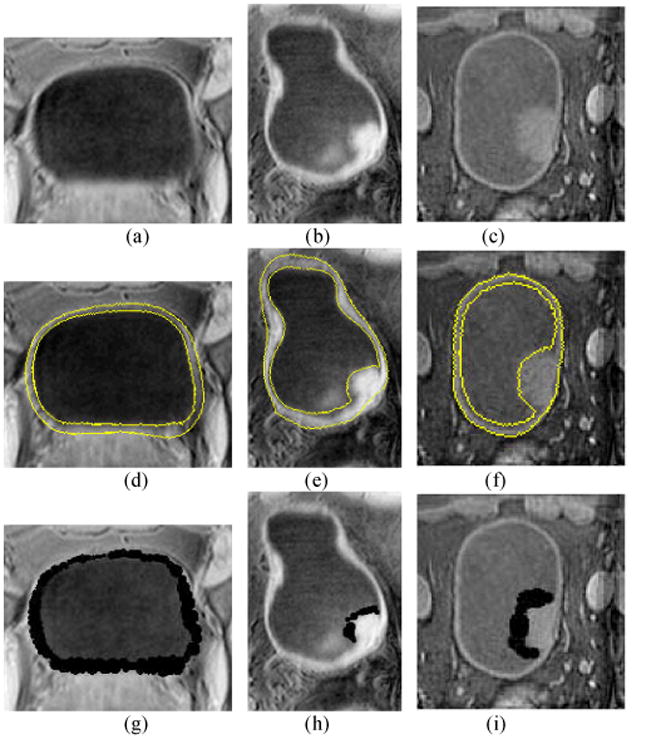
Example images to illustrate the window arrangement. The first, second and third rows show the original T₁-weighte MR images, the segmented results by the coupled level set method and the window arrangement, respectively. Each column is from the same slice of the same dataset. The left column is the image from a volunteer. The middle and right columns are two patient cases with a tumor in each case. The segmented inner and outer borders of the bladder wall on images (d)–(f) are highlighted by yellow curves. The black regions on images (g)–(i) are the overlapping windows. Picture (g) shows the window on the normal bladder wall. Pictures (h) and (i) show the windows covering the tumor surfaces.

C. Performance of the Candidates Detection

As described in Section V.A above, the candidates were detected by using the two geometry-related features, SI and NWT. The thresholds for each of these two operators are listed in Table III. Since the tumor head and tumor foot have the SI values close to 1.0 and 0.0, respectively, so we set two SI threshold intervals. The lower one was from 0.00 to 0.05 and the higher one from 0.95 to 1.00. The minimum value of NWT was set to be 1.1. The maximum value was open. The candidates included 223 TP windows and 3139 FP windows as listed in Table II. Totally 3362 candidate windows left after the two operators. Comparing with the original 10714 windows arranged on the inner borders of the ten datasets, the performance of the two operators was excellent. The 223 TPs indicate 100% coverage of the tumor surfaces by the windows in this step.

As mentioned above, previous work has proved that the bladder wall thickening is a clue for detecting the bladder tumors and can be measured by using CT images [15]. However, that work needs to map the bladder wall onto a uniform frame and applies statistical analysis using a large number of datasets. It further assumes that the thickness of normal bladder wall is similar from different subjects. This is an ill assumption in reality. The bladder shape and the wall thickness in our MR image database vary obviously because of the intrinsic variation from patient to patient and the different time points of data scanning. Among the 10 datasets used in this paper, the average wall thicknesses vary from 6 to 12 voxels. In other words, the wall thickness varies within each dataset and also varies among different datasets. Despite the latter variation among different datasets, the wall thickening is a sensitive parameter if the bladder walls scanned under different conditions can be normalized and re-parameterized on to a uniform framework. That is the reason the bladder wall thickness was normalized to generate the NWT.

However, the NWT brings uncertainties at the tumor foot where the thickness is similar to the normal bladder wall, and where the SI may contribute to the candidate extraction. Fig. 9 illustrates two phantoms, which simulate the bladder wall with tumors. The phantoms have the same resolution with the reformed T₁-weighted MR datasets used in this work. The plane is the bladder wall. Three protrusions represent tumors on the inner border. From left to right are two ball-shaped tumors with radii 5mm and 10mm, respectively. The third protrusion is an ellipsoid, which simulates a flatten tumor. Fig. 9(a) is rendered by the SI value while Fig. 9(b) uses the NWT. It is obviously that the NWT is effective to detect the bigger tumor (the middle one), and very possibly loses the smaller or flatten tumors. The tumor foot region and the normal bladder wall are not distinguishable in Fig. 9(b). However, the SI has a value close to 0.0 at the tumor foot and 1.0 at the tumor head, which makes the segmentation of the whole tumor surface possible. The color bars in Figs. 9(a)–(b) show the SI and NWT values, respectively.

Fig. 9.

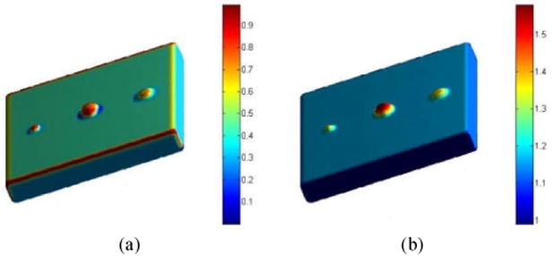
Two phantoms each with three tumors. The phantoms have the same resolution as the reformed T₁-weighed MR datasets used in this work. (a) The tumors rendered by the SI values. (b) The tumor rendered by the NWT values.

D. Evaluation of the Tumor Window Discriminant Strategy

To evaluate the performance of the features and the discriminant strategy QDA, both the ROC analysis and the free response ROC (fROC) analysis were applied. The ROC curves were used to measure the performance of different feature combinations in classifying the true tumor windows and the FPs. The fROC curve evaluated the overall performance of the tumor surface segmentation.

To generate the ROC, the threshold value t in Eq. (9) was used as the sweeping variable. The ROC curve was obtained and the area under the curve (AUC) was computed. Different feature combinations were tested. Table IV lists the results of several typical combinations. The combination in the first row outperformed all the other combinations and, therefore, was used for the following overall performance evaluation. The statistics-, geometry-, and layer-based features were applied separately and their performances are shown in the 2^nd, 3^rd and 4^th rows, respectively. The statistics-based features contributed the most to the FP reduction, which achieved a noticeable improvement over the former work of relying only on the geometry and wall thickness information. Fig. 10 depicts the ROC curves of different feature combinations.

Table IV. ROC Analysis of Different Feature Combinations.

Feature Combination	Area
1: All Features	0.95
2: Statistics	0.90
3: SI, NWT	0.88
4: Layer Derivatives	0.74

Fig. 10.

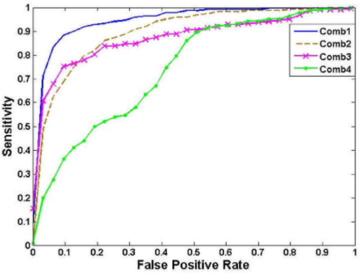
ROC curves generated from different feature combinations

The fROC was computed and displayed in Fig. 11 by using the feature combination 1. The vertical axis is the percentage of the true tumor surface covered by the detecting windows, 1.0 means the tumor surface labeled by the experts were completely covered by the windows. The FP per dataset is the FP number averaged to one dataset. One FP here means a region that consists of connective FP windows. Generally, we removed the regions smaller than 2mm which are considered as being generated by image noise [18-21]. Fig. 11 shows that 90% of the tumor surface was covered by the windows while 1.6 FPs per dataset were detected by mistake, and 100% surface was covered with 4.4 FPs per dataset. The areas under the windows were also measured. The average FP to TP surface area ratio is 0.38, where the surface area was computed by the inner border or the tumor surface covered by the windows. The lower two rows in Table I show the remaining FP window numbers after the QDA discrimination.

Fig. 11.

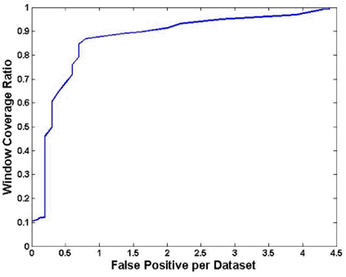
The fROC curve generated from the feature combination 1.

In Table V, more details were provided about the final results. The terms “Tumor D” and “Wall D” indicate the numbers of windows on the tumor and the normal bladder wall, respectively, as detected by our method. The “Tumor L” and “Wall L” show the numbers of tumor and wall windows labeled according to the experts' manual delineation (the ground truth). The percentages 50%, 90% and 100% in the 1^st column mean the detecting ratio of the true tumor windows. As shown in Table V, all the 223 true tumor windows were correctly detected with 117 (or FPs) out of 10374 normal wall window being detected as tumor window by mistake. If the detecting ratio lowers to 50%, then almost all FPs were excluded.

Table V. Confusion Matrix of the Final Window Distribution.

		Tumor D	Wall D
50%	Tumor L	110	113
	Wall L	3	10488
90%	Tumor L	198	25
	Wall L	19	10472
100%	Tumor L	223	0
	Wall L	117	10374

Three experts were also asked to score the results. The images were displayed with the remaining detecting windows under the 90% TP sensitivity. The scores mainly reflect how much the remaining windows can help them to find and locate the bladder tumor. In the procedure, the detected portion of the tumor surface was used as the intermediate results for the extraction of the tumor region and the analysis of the tumor features. Since the extraction and analysis operations were performed by the computer instead of the experts, therefore the expert scores provided here are only used as references. Table VI gives the mean scores from the three experts on the results of the ten datasets. The score spans from 0 to 10. Higher score means better performance. The scores of Table VI prove that the results are well accepted by the experts.

Table VI. Experts' Scores.

Dataset	1	2	3	4	5	6	7	8	9	10
Score	8.5	9.1	8.9	9.3	9.1	8.8	9.7	9.0	9.3	8.7

VII. Conclusion

This paper proposed an adaptive window-setting scheme to segment the entire bladder tumor surface with acceptable FP numbers. T₁-weighted MR images were used for that purpose due to its better bladder wall contrast, which provided the textures information for delicate analysis. Our previous coupled level set framework was employed to segment the inner and outer borders of the bladder wall simultaneously. Detecting windows with different radii were arranged on the inner border of the bladder wall. The window radius was adaptive to different bladder wall structures. The candidate windows were selected by using SI and NWT with predefined thresholds on an application-specific range. Statistics-, geometry- and layer-based features were extracted from the candidate windows. The QDA classifier was applied in the feature space to reduce the FP windows. Both ROC and fROC curves were generated to evaluate the performance of the classifier, feature combinations and the detection and segmentation procedure. This work was tested by ten clinical image datasets including five patients and five volunteers. Throughout the result report and associated discussion in the previous section, it can be observed that the bladder wall thickness and geometry features, such as the SI, are efficient for tumor detection, and the statistics of the in-window features are effective for classifying the tumor surface and the normal bladder wall surface. The layer derivatives add more necessary information for the classification. These features together provide the potential of detecting small and flattening tumors, which are hardly detected by the geometrical features individually. In summary, the results showed the effectiveness of the proposed method in detecting the bladder tumors and segmenting the whole surface of the detected bladder tumors.

In our future work, more effort will be devoted to acquire new clinical datasets from both patients and volunteers. The effectiveness and robustness of the current method need to be tested by more patient datasets including smaller tumors with different types. Based on the segmentation of the entire tumor surface, to further dig out the exact tumor regions inside the bladder wall and extract quantitative parameters from the tumor volume for computer-aided detection and diagnosis are under development. To integrate this work into a virtual cystoscopy system, further improvement on the accuracy of the detection and segmentation and the efficiency of computation will be needed and are under progress.

References

- 1.Bae KT, Kim JS, Na YH, et al. Pulmonary nodules: automated detection on CT images with morphologic matching algorithm-preliminary results. Radiology. 2005;236:286–294. doi: 10.1148/radiol.2361041286. [DOI] [PubMed] [Google Scholar]
- 2.Taylor SA, Halligan S, Burling D, et al. Computer-assisted reader software versus expert reviewers for polyp detection on CT colonography. American Journal of Roentgenology. 2006;186:696–702. doi: 10.2214/AJR.04.1990. [DOI] [PubMed] [Google Scholar]
- 3.Halligan S, Taylor SA, Dehmeshki J, et al. Computer-assisted detection for CT colonography: External validation. Clinical Radiology. 2006;61:758–763. doi: 10.1016/j.crad.2006.02.015. [DOI] [PubMed] [Google Scholar]
- 4.Liu F, Duan C, Yuan K, Liang Z, Bao S. Detecting bladder abnormalities based on inter-layer intensity curve for virtual cystoscopy. Proceedings of MICCAI 2010 Workshop: Virtual Colonoscopy & Abdominal Imaging. 2010;9:97–103. [Google Scholar]
- 5.Wu Z, Shi Z, Zhang G, Lu H. Detection of the invasion of bladder tumor into adjacent wall based on textural features extracted from MRI images. Proceedings of MICCAI 2010 Workshop: Virtual Colonoscopy & Abdominal Imaging. 2010;9:97–103. [Google Scholar]
- 6.Wingo PA, Tong T, Bolden S. Cancer statistics. A Cancer Journal for Clinicians. 1995;45:8–30. doi: 10.3322/canjclin.45.1.8. [DOI] [PubMed] [Google Scholar]
- 7.Lamm DL, Torti FM. CA: Bladder cancer. A Cancer Journal for Clinicians. 1996;46:93–112. doi: 10.3322/canjclin.46.2.93. [DOI] [PubMed] [Google Scholar]
- 8.Jemal A, Thomas A, Murray T, Thun M. Cancer statistics. A Cancer Journal for Clinicians. 2002;52:23–47. doi: 10.3322/canjclin.52.1.23. [DOI] [PubMed] [Google Scholar]
- 9.Jemal A, Siegel R, Ward E, Hao Y, Xu J, Murray T, Thun MJ. Cancer statistics. A Cancer Journal for Clinicians. 2008;58:71–96. doi: 10.3322/CA.2007.0010. [DOI] [PubMed] [Google Scholar]
- 10.American Cancer Society. Cancer Facts & Figures. 2008:4–10. [Google Scholar]
- 11.Overview: Bladder Cancer. [Retrieved June 8, 2010]; Online. Available: http://www.cancer.org.
- 12.Steiner GD, Trump DL, Cummings KB. Metastatic bladder cancer: Natural history, clinical course, and consideration for treatment. Urologic Clinics of North America. 1992;19:735–746. [PubMed] [Google Scholar]
- 13.Almallah YZ, Rennie CD, Stong J, Lancashire MJR. Urinary tract infection and patient satisfaction after flexible cystoscopy and urodynamic evaluation. Urology. 2000;56(no. 1):37–39. doi: 10.1016/s0090-4295(00)00555-0. [DOI] [PubMed] [Google Scholar]
- 14.Fielding JR, Hoyte L, Okon SA, et al. Tumor detection by virtual cystoscopy with color mapping of bladder wall thickness. The Journal of Urology. 2002;167:559–562. doi: 10.1016/S0022-5347(01)69085-2. [DOI] [PubMed] [Google Scholar]
- 15.Jaume S, Ferrant M, Macq B, Hoyte L, Fielding JR, Schreyer A, Kikinis R, Warfield SK. Tumor detection in the bladder wall with a measurement of abnormal thickness in CT scans. IEEE Transactions on Biomedical Engineering. 2003;50(no. 3):383–390. doi: 10.1109/TBME.2003.808828. [DOI] [PubMed] [Google Scholar]
- 16.Vining DJ, Zagoria RJ, Liu K, Stelts D. CT cystoscopy: An innovation in bladder imaging. American Journal of Roentgenology. 1996;166:409–410. doi: 10.2214/ajr.166.2.8553956. [DOI] [PubMed] [Google Scholar]
- 17.Liang Z, Chen D, Button T, Li H, Huang W. Feasibility studies on extracting bladder wall from MR images for virtual cystoscopy. Proc International Society of Magnetic Resonance in Medicine. 1999;3:2204. [Google Scholar]
- 18.Bernhardt TM, Rapp-Bernhardt U. Virtual cystoscopy of the bladder based on CT and MRI data. Abdominal Imaging. 2001;26:325–332. doi: 10.1007/s002610000168. [DOI] [PubMed] [Google Scholar]
- 19.Lämmle M, Beer A, Settles M, Hannig C, Schwaibold H, Drews C. Reliability of MR imaging-based virtual cystoscopy in the diagnosis of cancer of the urinary bladder. American Journal of Roentgenology. 2002;178:1483–1488. doi: 10.2214/ajr.178.6.1781483. [DOI] [PubMed] [Google Scholar]
- 20.Bernhardt TM, Schmidl H, Philipp C, Allhoff EP, Rapp-Bernhardt U. Diagnostic potential of virtual cystoscopy of the bladder: MRI v.s. CT. Preliminary report. European Radiology. 2003;13:305–312. doi: 10.1007/s00330-002-1444-9. [DOI] [PubMed] [Google Scholar]
- 21.Browne RF, Murphy SM, Grainger R, et al. CT cystography and virtual cystoscopy in the assessment of new and recurrent bladder neoplasms. European Journal of Radiology. 2005;53:147–153. doi: 10.1016/j.ejrad.2004.02.002. [DOI] [PubMed] [Google Scholar]
- 22.Li L, Wang Z, Harrington D, Huang W, Liang Z. A mixture-based computer aided detection system for virtual cystoscopy. Proc International Society of Magnetic Resonance in Medicine. 2003:1466. [Google Scholar]
- 23.Zhu H, Duan C, Jiang R, Li L, Fan Y, Yu X, Zeng W, Gu X, Liang Z. Computer-aided detection of bladder tumors based on the thickness mapping of bladder wall in MR images. Proc SPIE Medical Imaging 2010, in CD-ROM [Google Scholar]
- 24.Duan C, Tian Z, Liang Z, et al. Segmenting bladder wall and estimating wall thickness for magnetic resonance virtual cystoscopy. Journal of Tsinghua University. 2010;50(no. 9):1445–1448. [Google Scholar]
- 25.Duan C, Yuan K, Bao S, Liang Z. Bent rate based bladder lesion enhancement with application to MR Cystography. ICIC Express Letters. 2010;4(no. 6B):2425–2429. [Google Scholar]
- 26.Duan C, Yuan K, Liu F, Xiao P, Lv G, Liang Z. Volume-based features for detection of bladder wall abnormal region via MR cystography. IEEE Transactions on Biomedical Engineering. 2011;58(no. 9):2506–2512. doi: 10.1109/TBME.2011.2158541. [DOI] [PMC free article] [PubMed] [Google Scholar]
- 27.Duan C, Liang Z, Bao S, et al. A coupled level set framework for bladder wall segmentation with application to MR cystography. IEEE Transactions on Medical Imaging. 2010;29(no. 3):903–915. doi: 10.1109/TMI.2009.2039756. [DOI] [PMC free article] [PubMed] [Google Scholar]
- 28.Li L, Wang Z, Li X, Wei X, Adler H, Huang W, Rizvi S, Meng H, Harrington D, Liang Z. A new partial volume segmentation approach to extract bladder wall for computer aided detection in virtual cystoscopy. Proc SPIE Medical Imaging. 2004;5369:199–206. [Google Scholar]
- 29.Li L, Liang Z, Wang S, Lu H, Wagshul M, Zawin M, Posniak E, Lee C. Segmentation of multi-spectral bladder MR images with inhomogeneity correction for virtual cystoscopy. Proc SPIE Medical Imaging, in CD-ROM. 2008 [Google Scholar]
- 30.Osher S, Sethian J. Fronts propagating with curvature dependent speed: Algorithms based on Hamilton-Jacobi formulation. Journal of Computational Physics. 1988;79:12–49. [Google Scholar]
- 31.Chan T, Vese L. Active contours without edges. IEEE Transactions on Image Processing. 2001;10(no. 2):266–277. doi: 10.1109/83.902291. [DOI] [PubMed] [Google Scholar]
- 32.Monga O, Benayoun S. Using partial derivatives of 3D images to extract typical surface features. Computer Vision and Image Understanding. 1995;61(no. 2):171–189. [Google Scholar]
- 33.Zhu H, Duan C, Pickhardt P, Wang S, Liang Z. Computer-aided detection of colonic polyps with level set-based adaptive convolution in volumetric mucosa to advance CT colonography toward a screening modality. Cancer Management and Research. 2009;1:1–13. doi: 10.2147/cmar.s4546. [DOI] [PMC free article] [PubMed] [Google Scholar]
- 34.Fukunaga K. Introduction to Statistical Pattern Recognition. San Diego: Academic Press; 1990. [Google Scholar]