Climate forcings in the Industrial era

Abstract

The forcings that drive long-term climate change are not known with an accuracy sufficient to define future climate change. Anthropogenic greenhouse gases (GHGs), which are well measured, cause a strong positive (warming) forcing. But other, poorly measured, anthropogenic forcings, especially changes of atmospheric aerosols, clouds, and land-use patterns, cause a negative forcing that tends to offset greenhouse warming. One consequence of this partial balance is that the natural forcing due to solar irradiance changes may play a larger role in long-term climate change than inferred from comparison with GHGs alone. Current trends in GHG climate forcings are smaller than in popular “business as usual” or 1% per year CO₂ growth scenarios. The summary implication is a paradigm change for long-term climate projections: uncertainties in climate forcings have supplanted global climate sensitivity as the predominant issue.

A climate forcing is an imposed perturbation of the Earth’s energy balance with space (1). Examples are a change of the solar radiation incident on the planet or a change of CO₂ in the Earth’s atmosphere. The unit of measure is Watts per square meter (W/m²), e.g., the forcing due to the increase of atmospheric CO₂ since pre-Industrial times is approximately 1.5 W/m² (2, 3).

Climate change is a combination of deterministic response to forcings and chaotic fluctuations—the chaos being a consequence of the nonlinear equations governing the dynamics of the system (4). Quantitative knowledge of all significant climate forcings is needed to establish the contribution of deterministic factors in observed climate change and to predict future climate.

We provide a perspective on current understanding of global climate forcings, in effect an update of the Intergovernmental Panel on Climate Change (IPCC; ref. 2). We stress the need for a range of forcing scenarios in climate simulations.

Greenhouse Gases (GHGs)

GHGs absorb and emit infrared (heat) radiation. Because temperature decreases with height in the Earth’s troposphere, increasing GHGs cause emission to space to arise from higher, colder levels, thus reducing radiation to space. This temporary imbalance with incoming solar energy forces the planet to warm until energy balance is restored.

Well-Mixed Gases.

Changes of long-lived GHGs during the Industrial era are known accurately. These gases are reasonably well-mixed in the troposphere, and thus their changes can be monitored at a small number of locations. The principal GHGs have been measured in situ for the past few decades and their pre-Industrial abundances can be determined from ancient air bubbles trapped in polar ice sheets (5).

Abundances of the principal human-influenced GHGs—CO₂, CH₄, N₂O, CFC-11, and CFC-12—are shown in Fig. 1. We estimate chlorofluorocarbon (CFC) amounts before the first measurements by using Industrial production data and assuming atmospheric lifetimes of 50 and 100 years for CFC-11 and CFC-12, respectively. The early records of the other gases are based on ice core data (6, 7). Tabular data for Fig. 1 are available at www.giss.nasa.gov/data/GHgases.

Figure 1.

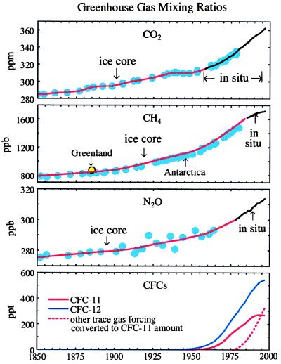
Principal anthropogenic GHGs in the Industrial era.

Climate forcings due to these trace gases can be computed accurately because the absorption properties are known within ≈10%. Analytic fits to calculations based on the correlated k-distribution method (8) are given in Table 1. The accuracies are believed to be within 10% for abundances occurring in the Industrial era, including plausible amounts in the next century.

Table 1.

Radiative forcings in industrial era

Gas	Radiative forcing
CO2	F = f(c) − f(c0), where f(c) = 5.04 ln[c + 0.0005c2]
CH4	0.04 (√m − √m0) − [g(m, n0) − g(m0, n0)] g(m, n) = 0.5 ln[1 + 0.00002(mn)0.75]
N2O	0.14 (√n − √n0) − [g(m0, n) − g(m0, n0)]
CFC-11	F = 0.25 (x − x0)
CFC-12	F = 0.30 (y − y0)

c, CO₂ (ppm); m, CH₄ (ppb); x, CFC-11 (ppb); and y, CFC-12 (ppb). 

The total climate forcing by the well-mixed GHGs in the Industrial era is ≈2.3 W/m² (Fig. 2). The forcing by CFCs includes an estimate of 0.1 W/m² for minor trace gases, which are mainly halocarbons (9, 10).

Figure 2.

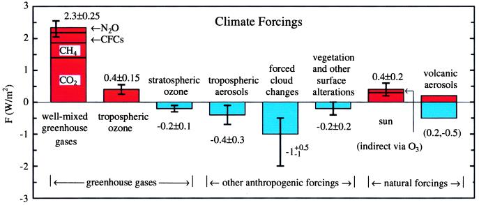
Estimated radiative forcings between 1850 and the present.

Inhomogeneously Mixed Gases.

Climate forcing by ozone is uncertain because ozone change as a function of altitude is not well measured. Ozone changes during the Industrial era include long-term tropospheric ozone increase associated with air pollution as well as stratospheric ozone depletion associated with anthropogenic chlorine and bromine emissions.

Surface ozone over Europe increased by a factor of five in the past century (11), but measurements cover a small region and calibration of early data is uncertain. Thus estimates of global tropospheric ozone change depend in part on chemistry models (12), which yield an ozone change in Europe smaller than that reported (11). We calculate a global forcing of 0.3 W/m² for the modeled tropospheric ozone change of the past century, based on an accurate radiative treatment (8) including realistic global distributions of clouds and other radiative constituents. Our estimated forcing and uncertainty in Fig. 2, 0.4 ± 0.15 W/m², reflect the range of data and models.

Ozone loss in recent years in the lower stratosphere and tropopause region, labeled “stratospheric” in Fig. 2 and derived from the most recent versions of satellite analyses, causes a climate forcing −0.2 ± 0.1 W/m² (13, 14). This negative forcing tends to offset the positive forcing due to increasing low level ozone. But this offset does not imply that ozone change has no climatic effect. Indeed, ozone change has a large effect on the temperature profile in the troposphere and stratosphere (13).

Climate forcing by stratospheric water vapor is not included in Fig. 2 because it is small and water vapor change is measured globally only for the past few years (15). Tropospheric water vapor, the strongest GHG, is not included either because this water vapor amount is a function of climate and thus represents a climate feedback, rather than a forcing (16).

Other Anthropogenic Forcings

In principal, there are any number of anthropogenic climate forcings in addition to GHGs. But forcings are likely to be important only if they involve change of one of the other major atmospheric radiative constituents, i.e., aerosols or clouds, or changes of the Earth’s surface. In fact, there appear to be significant changes of all three of these factors.

Aerosols.

Aerosols are fine particles suspended in the air. There are many aerosol sources and compositions (2, 17, 18). The anthropogenic component of atmospheric aerosols still is poorly known and thus so is the aerosol climate forcing.

Our quantitative evaluation focuses on three aerosols that probably contribute most to the anthropogenic aerosol optical depth: sulfates, organic aerosols, and soil dust. But we use realistic aerosol absorption, and thus we also implicitly include the principal radiative effect of minor aerosol constituents such as black carbon (soot).

Aerosol optical depth τ is defined such that a vertically incident solar beam is attenuated by the factor exp(−τ). Aerosol absorption effects are represented by the aerosol single scatter albedo ω. ω is the fraction of sunlight intercepted by the aerosol that is scattered (i.e., not absorbed).

Sulfate is the aerosol that has received most attention. The principal anthropogenic source is sulfur in fossil fuels, which is emitted as SO₂ during combustion and oxidized in the atmosphere to become mainly sulfuric acid. Fig. 3A shows the annual global distribution of fossil fuel sulfate derived from a chemical transport model (19).

Figure 3.

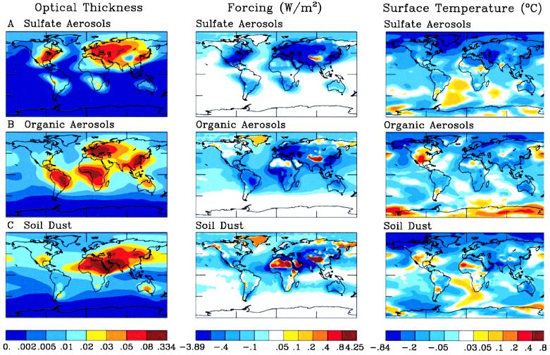
Optical depth, climate forcing, and simulated equilibrium temperature change for three assumed anthropogenic aerosol distributions. These are the three “more realistic” single scatter albedo (ω) cases of Table 2.

Organic aerosols, i.e., aerosols containing organic carbon, are produced in combustion of biomass and fossil fuels (2, 17, 20, 21). The global distribution of organic aerosols is not well known, but field studies find them to be a large portion of total aerosol amount (22). Fig. 3B shows an estimated global distribution of anthropogenic organic aerosols (20), with the aerosols in Eurasia and North America based on fossil fuel sources and those at low latitudes and in the Southern Hemisphere associated with biomass burning.

Soil (mineral) dust aerosols are produced mainly in arid and semi-arid regions, especially when the soil or vegetation is disturbed. Fig. 3C shows an estimated global distribution of anthropogenic soil dust based on an atmospheric transport model (23) with several regions of land-use disturbance.

These three aerosols may dominate anthropogenic aerosol optical depth, but the climate forcing also depends strongly on minor constituents, especially black carbon. In principal, the absorption and scattering of all constituents can be added to produce the total τ and ω that, along with the aerosol angular scattering pattern, determine the radiative effect. But this approach yields a huge uncertainty in the climate forcing. One difficulty is that ω is sensitive to whether black carbon is externally mixed or contained within the dominant aerosols (24) because internal mixing of black carbon increases its absorptive effect. ω and τ also vary with humidity.

These difficulties suggest the need to use observations more directly related to the forcing, especially for the net ω. In situ observations of ω (25) confirm substantial, but highly variable, aerosol absorption. Assessment of aerosol forcing probably requires advanced capabilities for global satellite measurement of aerosol scattering and absorption properties (26).

In the interim, aerosol forcing can be estimated by using climate model calculations with a range of values for ω. Table 2 gives the aerosol forcing and mean global temperature change in the last 20 years of 50 year simulations with a global climate model (13) that used conservatively scattering (ω = 1) and absorbing aerosols. Absorbing aerosols had ω = 0.95 for “sulfates”, ω = 0.92 (21) for “organics”, and a wavelength dependent ω appropriate for soil dust (27). Calculated forcings vary linearly in τ and (1 − ω) for plausible changes of τ or ω.

Table 2.

Global mean forcings for three aerosol types

Aerosol	ω = 1		“More realistic” ω
	ΔF(W/m2)	ΔTs(C)	ΔF(W/m2)	ΔTs(C)
“Sulfate”	−0.28	−0.19	−0.20	−0.11
Organic	−0.41	−0.25	−0.22	−0.08
Dust	−0.53	−0.28	−0.12	−0.09
Total	−1.22	−0.72	−0.54	−0.28

The regional patterns of climate response (Fig. 3) bear only crude resemblance to the geographical distribution of aerosols. This is a result of both the chaotic variability of climatic patterns and the fact that changes in atmospheric and surface heating alter atmospheric dynamics (28).

We estimate anthropogenic aerosol forcing as −0.4 ± 0.3 W/m², slightly less negative than the “more realistic” ω case in Table 2. Reasons for this choice are that ω = 0.95 for sulfates plus black carbon may understate the absorption (24, 25) and our annual global mean optical depth of anthropogenic organic aerosols (0.02) may be too high. Also soil dust forcing varies with choice of aerosol size and altitude distribution, and it can yield even a small positive forcing (3, 27). Aerosol forcing will remain very uncertain until better observations are obtained.

Clouds.

Anthropogenic cloud changes are a potentially larger climate forcing than direct aerosol effects, but they are even more uncertain. Most forced cloud changes, including aircraft contrails, are an indirect effect of anthropogenic aerosols. Aerosols serve as condensation nuclei for clouds, and thus added aerosols alter the cloud-drop size distribution. An increase of aerosols yields smaller cloud-drops, thus a larger cloud albedo (29), but it also increases cloud cover by inhibiting rainfall and thereby increasing cloud lifetime (30).

We consider two ways to estimate climate forcing by clouds. The first method is based on aerosol-cloud modeling. The second approach is an inference of the forcing from observed changes in the diurnal cycle of surface air temperature.

Aerosol-cloud models yield a range of estimates for cloud forcing. A typical result is approximately −1 W/m², but it varies by an order of magnitude as model parameters are varied within their uncertainties (31). Most models examine only sulfates, which may dominate the indirect aerosol effect because they are so hygroscopic. But mineral and carbonaceous aerosols influence cloud condensation, often being coated with a small amount of sulfuric acid, adding further uncertainty to aerosol-cloud forcing. Thus aerosol models have been fruitless, as far as providing a useful constraint on cloud forcing is concerned.

A second estimate of radiative forcing by clouds is based on damping of the diurnal cycle of surface temperature that has occurred over much of the world (32). Mechanisms that damp the local diurnal cycle include increase of soil moisture and increase of atmospheric aerosols, but quantitative analysis shows that these mechanisms are unable to account for the large observed global-scale damping (33). The only mechanism found to cause such a large global-scale effect is increased cloud cover, with the increase being mainly in the Northern Hemisphere. Increased clouds damp the diurnal cycle by decreasing solar heating of the surface in the day and decreasing surface cooling to space at night. Increased aerosols contribute a small amount to diurnal damping via the same mechanisms.

Climate simulations agree best with the observed diurnal cycle change if the forcing, due to both clouds and aerosols, is between −1 and −1.5 W/m² (33). If the aerosol forcing is only a few tenths of −1 W/m², as estimated above, this implies a cloud forcing of approximately −1 W/m². This method of obtaining the cloud forcing is a good approach because the radiative mechanisms causing cloud forcing and diurnal damping, discussed above, are closely related. A cloud’s effectiveness for climate forcing and diurnal damping varies with the cloud altitude, but relatively low clouds appear to dominate both the cloud forcing and diurnal damping (1, 33).

Observations of cloud cover and sunlight duration suggest that cloud cover has increased this century (34), although data accuracy and coverage are poor. It has been suggested that the cloud increase could be a cloud feedback accompanying global warming (35). But in doubled CO₂ and transient climate simulations (13), we find that the cloud changes accompanying an 0.5°C global warming, based on a state-of-the-art cloud simulation (36), have an impact on the diurnal cycle an order of magnitude smaller than that observed. Thus, we conclude that the observed cloud increase is probably an indirect effect of aerosols, rather than a climate feedback.

Based on the inference that clouds are the cause of the observed change of the diurnal cycle of surface temperature, we estimate that the aerosol-cloud forcing is −1 W/m² for the Industrial era with a factor of two uncertainty. The asymmetric uncertainty acknowledges the possibility of cloud forcing introduced before diurnal cycle data, but most of the aerosol-cloud forcing was probably added during the growth of fossil fuel use in 1945–1980 (see below). Confirmation of the aerosol-cloud forcing requires a coordinated research program including accurate global measurement of aerosol and cloud changes, as well as in situ field studies and aerosol modeling.

Land-Use.

The principal change imposed on the Earth’s surface during the Industrial era is probably land-use changes, including deforestation, desertification, and cultivation. Land-use changes alter the albedo (reflectivity) of the surface and modify evapotranspiration and surface roughness. One large effect of altered vegetation occurs via the impact of snow on albedo. The albedo of a cultivated field, e.g., is affected more by a given snowfall than is the albedo of an evergreen forest.

We carried out a climate simulation with pre-Industrial vegetation replaced by current land-use patterns (37). In this experiment, cropland is approximated as having the properties of grassland and deforested tropical land undergoing regrowth is treated as woodland. The global climate forcing due to current land-use, i.e., the change in the planetary radiation balance, is −0.21 W/m², with the largest contributions from deforested areas in Eurasia and North America (Fig. 4 Left).

Figure 4.

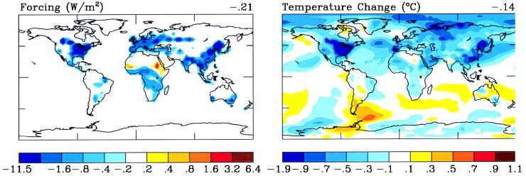
Climate forcing and simulated surface air temperature response for land-use change between the pre-Industrial era and the present.

The simulated climate response to this forcing has global cooling of 0.14°C (Fig. 4 Right). The dominant effect is increased albedo in regions of deforestation subject to snowfall, which apparently overwhelms other effects such as warming due to reduced evapotranspiration. However, this result is only an initial estimate for the climate effect of anthropogenic land-use.

Some land-use change, e.g., in China, occurred centuries ago, but there are also areas of change not included in our data set. Thus we take global land-use climate forcing as −0.2 W/m² with uncertainty 0.2 W/m² (Fig. 2). Improved determination requires comprehensive historical data on land-use change and increased realism of land processes in climate models.

Natural Forcings

Natural climate forcings are limited to factors “imposed” on the climate system. Thus fluctuations of soil dust aerosols that occur with drought conditions are an internal climate feedback process. The dominant known natural climate forcings that may be important on global and decadal time scales are changes of the sun and stratospheric aerosols from large volcanoes. Both of these forcings have been measured accurately from satellites during the past two decades and are estimated for the preceding century from indirect measures.

Solar Irradiance.

Measured changes of solar irradiance since 1979 reveal a cyclic variation of amplitude ≈0.1% in phase with the sunspot cycle (38). The variation is largest at UV wavelengths that are absorbed in the stratosphere, but ≈85% of the variation occurs at wavelengths that penetrate into the troposphere.

Variations of solar irradiance on longer time scales are hypotheses based on ad hoc relationships between irradiance and observed solar features such as sunspot number or the length of the solar cycle. The estimated solar forcing of 0.3 W/m² for the period 1850 to the present (Fig. 2) is based on the analysis of Lean et al. (39).

Additional indirect solar forcings have been hypothesized, but so far only a small effect via ozone changes has been quantified. The indirect solar forcing via ozone change is in phase with the direct solar forcing and approximately one-third of its magnitude (1). Thus, this indirect solar effect may have added a positive forcing of ≈0.1 W/m² over the past 150 years.

Volcanos.

Stratospheric aerosols from large volcanoes can cause a large negative forcing. This forcing decays approximately exponentially with a time constant of ≈1 year. The eruption of Mt. Pinatubo in 1991, which caused a peak forcing just over 3 W/m² with an uncertainty of ≈20% (13), was probably the largest volcanic aerosol forcing this century.

The climate forcing due to volcanoes in the century preceding satellite data can be estimated from measurements of atmospheric transparency (40). But, because of limitations in the spatial, temporal, and spectral coverage of these ground-based data, the accuracy of the global climate forcing is probably not better than a factor of two.

We calculate the decadal mean of this episodic forcing because our interest is long-term climate change. Fig. 2 shows the range of volcanic aerosol forcings between a decade with no large volcanoes and the decade estimated to have the greatest aerosol amount during the past 150 years (the 1880s). The forcings are calculated relative to the mean aerosol forcing for the period since 1850 (40). Note that use of the decadal mean for this episodic forcing differs from the other forcings in Fig. 2, which each represent the change since 1850.

Climate Forcings and Response: A Paradigm Change

The principal climate change issue of the past two decades, exemplified by the Charney (41) report, was climate sensitivity. That report estimated global climate sensitivity as near 3°C for doubled atmospheric CO₂ with a probable error of ±1.5°C. The large uncertainty is a result of poorly understood climate feedbacks, especially clouds and water vapor.

In the past 20 years, remarkable advances in paleoclimate data have constrained climate sensitivity (5). The causes and sequences of long-term climate change remain controversial, but the large changes in planetary surface conditions and atmospheric composition that maintained global energy balance are well known. Specifically, it has been shown that the 5°C global climate change between the last ice age and the current interglacial period was maintained by a global forcing of 7.5 ± 1.5 W/m² (16, 42, 43). Speculation that change of ocean poleward heat transport maintained the ice age cold was disproved by reconstructions of substantial cooling at all latitudes.

The result is confirmation that climate is very sensitive to global radiative forcings; we estimate, 3 ± 1°C for doubled CO₂. Crucial climate sensitivity issues remain, e.g., the possibility of a climate threshold for collapse of the ocean’s thermohaline circulation (44). Yet it seems clear that the prime issue now has become climate forcings, i.e., there is greater uncertainty in future climate forcings than in global mean climate sensitivity.

GHGs.

The growth rate of GHG climate forcing is shown in Fig. 5. Between 1950 and the early 1970s, the growth rate rocketed from 0.01 to 0.04 W/m²/yr, driven by exponential 4.6%/yr growth of fossil fuel CO₂ emission (Fig. 6). In the last 20 years, the growth rate leveled out and declined to ≈0.03 W/m²/yr due to a flattening of the CO₂ growth rate and plummeting growth rates for CFCs and CH₄ (9). Cumulative greenhouse forcing is continuing to increase rapidly, at a rate that would cause doubled CO₂ forcing in approximately one century, but the altered rate emphasizes the need to understand the changes, and it increases the importance of comparison of the greenhouse forcing with other forcings (Fig. 2).

Figure 5.

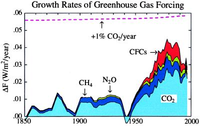
Growth rate of greenhouse climate forcing based on gas histories shown in Fig. 1. Dashed line is forcing due to 1% CO₂ increase.

Figure 6.

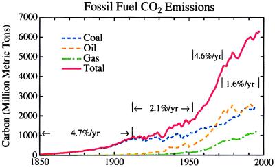
Fossil fuel CO₂ emissions (45). Mean annual growth rates are shown for four periods.

We showed individual GHG growth rates elsewhere, which raises several questions (9). Why has the CO₂ growth rate flattened despite continued increase of fossil fuel emissions, albeit at a slower growth rate; is this a long-term increase in a carbon sink or a temporary biospheric uptake presaging a later burst of CO₂ growth? Is the reduced CH₄ growth rate temporary or is there an opportunity for further decline and even a partial balancing of CO₂ growth? CH₄ is responsible for a large fraction of the anthropogenic greenhouse effect, and seems susceptible to change, but has not received commensurate attention. The role of O₃ changes is not well known because of the absence of accurate knowledge of changes in its vertical profile.

Aerosols and Clouds.

The present climate forcing by anthropogenic aerosols, the direct effect plus the impact on clouds, is probably large and negative, at least −1 W/m². But because of the short lifetime of aerosols, the forcing depends on their current rate of emission, not on prior emissions. It is likely that during the 1975–98 era of slow growth of fossil fuels, when also the sulfur fraction of fuels was being reduced in some countries, that there was little change in global aerosol forcing. Thus it is not surprising that climate simulations for the satellite era (13) achieve close agreement with observations without any tropospheric aerosol changes.

Most of the current direct and indirect aerosol forcing must have been introduced during the era of rapid fossil fuel growth, 1950–75. Such aerosol forcing, say −1 W/m², would approximately balance, on global average, increased greenhouse forcing in the same era. This partial balance of forcings may account for the lack of strong global temperature change in that era. Paradoxically, it was probably the slowdown of fossil fuel growth rates in the last 25 years that allowed greenhouse warming to dominate over aerosol cooling and a strong global warming trend to emerge.

This interpretation emphasizes the need for measurements of the aerosol and cloud forcings. This follows also from Fig. 2, which shows that the uncertainty in the net climate forcing is dominated by the uncertainty in the forced cloud changes. It is noteworthy that at present there is no major research program focused on accurately defining this latter forcing.

Land-Use.

Land-use climate forcing, not included by IPCC (2), needs more attention. Our preliminary analysis indicates that it is a minor global cooling factor, as increased albedo in snowy regions exceeds the effect of reduced evaporative cooling of low latitude deforestation. But improved assessments, based on better input data and increased realism of land surface processes in climate models, are needed.

Solar Irradiance.

Sometimes it is argued that climate forcing due to solar variability is negligible because it is much smaller than the GHG forcing. However, a more relevant comparison is with the net forcing by all other known mechanisms. Fig. 2 suggests that this net forcing may be only ≈1 W/m², with considerable uncertainty. Thus a solar forcing of even 0.4 W/m² could have played a substantial role in climate change during the Industrial era. If solar irradiance is now at a relatively high level, as some evidence suggests (39), solar forcing could be negatve in the coming century, thus tending to counteract GHG forcing rather than reinforcing it (Fig. 2). This emphasizes our need to monitor and understand solar variability.

Scenarios.

Climate forcing scenarios are essential for climate predictions, including communications with the public about potentially dangerous climate changes (46, 47). But if only one forcing scenario is used in climate simulations, as has been a recent tendency, the scenario itself is likely to be taken as a prediction, as well as the calculated climate change. Moreover, the single scenarios tend to be “business as usual” or 1% CO₂/yr forcings, which are approximately double the actual current climate forcings. As one of the purposes of simulations is to allow consideration of options for less drastic change, and as there is large uncertainty in present and future forcings, we recommend the use of multiple scenarios. This will aid objective analysis of climate change as it unfolds in coming years.

ABBREVIATIONS

GHG

greenhouse gas

CFC

chlorofluorocarbon

References

- 1. Hansen J, Sato M, Ruedy R. J Geophys Res. 1997;102:6831–6864. [Google Scholar]
- 2.Houghton J T, Meira Filho L G, Callander B A, Harris N, Kattenberg A, Maskell K, editors. Intergovernmental Panel on Climate Change. Climate Change (1995) Univ. Press, Cambridge, U.K.: Cambridge; 1996. [Google Scholar]
- 3.Hansen J, Sato M, Lacis A, Ruedy R. Philos Trans R Soc London B. 1997;352:231–240. [Google Scholar]
- 4.Lorenz E N. J Atmos Sci. 1963;20:130–141. [Google Scholar]
- 5.Lorius C, Jouzel J, Raynaud D, Hansen J, Le Treut H. Nature (London) 1990;347:139–145. [Google Scholar]
- 6.Etheridge D M, Steele L P, Francey R J, Langenfelds R L. J Geophys Res. 1998;103:15979–15993. [Google Scholar]
- 7.Machida T, Nakazawa T, Fujii Y, Aoki S, Watanabe O. Geophys Res Lett. 1995;22:2921–2924. [Google Scholar]
- 8.Lacis A A, Oinas V. J Geophys Res. 1991;96:9027–9064. [Google Scholar]
- 9.Hansen J, Sato M, Glascoe J, Ruedy R. Proc Natl Acad Sci USA. 1998;95:4113–4120. doi: 10.1073/pnas.95.8.4113. [DOI] [PMC free article] [PubMed] [Google Scholar]
- 10.Myhre G, Highwood E J, Shine K P, Stordal F. Geophys Res Lett. 1998;25:2715–2718. [Google Scholar]
- 11.Marenco A, Gouget H, Nedelec P, Pages J-P, Karcher F. J Geophys Res. 1994;99:16617–16632. [Google Scholar]
- 12.Crutzen P J. In: Low Temperature Chemistry of the Atmosphere. Moortgat G K, Barnes A J, Le Bras G, Sodeau J R, editors. Berlin: Springer; 1994. pp. 465–498. [Google Scholar]
- 13.Hansen J, Sato M, Ruedy R, Lacis A, Asamoah K, Beckford K, Borenstein S, Brown E, Cairns B, Carlson B, et al. J Geophys Res. 1997;102:25679–25720. [Google Scholar]
- 14.de Forster P M, Shine K P. J Geophys Res. 1997;102:10841–10855. [Google Scholar]
- 15.Evans S J, Toumi R, Harries J E, Chipperfield M P, Russell J M. J Geophys Res. 1998;103:8715–8725. [Google Scholar]
- 16.Hansen J, Lacis A, Rind D, Russell G, Stone P, Fung I, Ruedy R, Lerner J. In: Climate Processes and Climate Sensitivity. Hansen J E, Takahashi T, editors. Vol. 29. Washington, DC: AGU; 1984. pp. 130–163. [Google Scholar]
- 17.Andreae M. In: World Survey of Climatology. Henderson-Sellers A, editor. Vol. 16. Amsterdam: Elsevier; 1995. pp. 347–398. [Google Scholar]
- 18.Charlson R J. Ambio. 1997;26:17–24. [Google Scholar]
- 19.Chin M, Jacob D J. J Geophys Res. 1996;101:18691–18699. [Google Scholar]
- 20.Liousse C, Penner J E, Chuang C, Walton J J, Eddlelman H. J Geophys Res. 1996;103:6043–6058. [Google Scholar]
- 21.Penner J E, Dickinson R E, O’Neill C A. Science. 1992;256:1432–1434. doi: 10.1126/science.256.5062.1432. [DOI] [PubMed] [Google Scholar]
- 22.Hegg D A, Livingston J, Hobbs P V, Novakov T, Russell P. J Geophys Res. 1997;102:25293–25303. [Google Scholar]
- 23.Tegen I, Fung I. J Geophys Res. 1995;100:18707–18726. [Google Scholar]
- 24.Haywood J M, Shine K P. Geophys Res Lett. 1995;22:603–606. [Google Scholar]
- 25.Ogren J. In: Aerosol Forcing of Climate. Charlson R J, Heintzenberg J, editors. New York: Wiley; 1995. pp. 215–226. [Google Scholar]
- 26.Hansen J, Rossow W, Carlson B, Lacis A, Travis L, Del Genio A, Fung I, Cairns B, Mishchenko M, Sato M. Clim Change. 1995;31:247–271. [Google Scholar]
- 27.Tegen I, Lacis A A, Fung I. Nature (London) 1996;380:419–422. [Google Scholar]
- 28.Miller, R. L. & Tegen, I. (1998) J. Climate, in press.
- 29.Twomey S A. Atmos Environ. 1991;25A:2435–2442. [Google Scholar]
- 30.Albrecht B A. Science. 1989;245:1227–1230. doi: 10.1126/science.245.4923.1227. [DOI] [PubMed] [Google Scholar]
- 31.Pan W, Tatang M A, McRae G J, Prinn R G. J Geophys Res. 1998;103:3815–3823. [Google Scholar]
- 32.Karl T R, Jones P D, Knight R W, Kukla G, Plummer N, Razuvayev V, Gallo K P, Lindseay J, Charlson R J, Peterson T C. Bull Am Meteorol Soc. 1993;74:1007–1023. [Google Scholar]
- 33.Hansen J, Sato M, Ruedy R. Atmos Res. 1995;37:175–209. [Google Scholar]
- 34.Henderson-Sellers A. Geol J. 1992;27:255–262. [Google Scholar]
- 35.Dai A, Del Genio A D, Fung I. Nature (London) 1997;386:665–666. [Google Scholar]
- 36.Del Genio A D, Yao M S, Kovari W, Lo K K W. J Climate. 1996;9:270–304. [Google Scholar]
- 37.Matthews E. J Clim Appl Meteorol. 1983;22:474–487. [Google Scholar]
- 38.Willson R C, Hudson H S. Nature (London) 1991;351:42–44. [Google Scholar]
- 39.Lean J, Beer J, Bradley R. Geophys Res Lett. 1995;22:3195–3198. [Google Scholar]
- 40.Sato M, Hansen J, McCormick M P, Pollack J B. J Geophys Res. 1993;98:22,987–22,994. [Google Scholar]
- 41.Charney J. Carbon Dioxide and Climate. Washington, DC: Natl. Acad. Press; 1979. [Google Scholar]
- 42.Hoffert M I, Covey C. Nature (London) 1992;360:573–576. [Google Scholar]
- 43.Hansen J, Lacis A, Ruedy R, Sato M, Wilson H. Natl Geograph Res Explor. 1993;9:142–158. [Google Scholar]
- 44.Manabe S, Stouffer R J. Nature (London) 1995;378:165–167. [Google Scholar]
- 45.Marland G, Boden T. CO2 Infor. Center. Oak Ridge, TN: Oak Ridge Natl. Lab.; 1998. , [Google Scholar]
- 46.Suplee C, Pinneo J B. Natl Geogr. 1998;193:69. [Google Scholar]
- 47.Shindell D T, Rind D, Lonergan P. Nature (London) 1998;392:589–592. [Google Scholar]