A Partitioning Based Adaptive Method for Robust Removal of Irrelevant Features from High-dimensional Biomedical Datasets

Abstract

We propose a novel method called Partitioning based Adaptive Irrelevant Feature Eliminator (PAIFE) for dimensionality reduction in high-dimensional biomedical datasets. PAIFE evaluates feature-target relationships over not only a whole dataset, but also the partitioned subsets and is extremely effective in identifying features whose relevancies to the target are conditional on certain other features. PAIFE adaptively employs the most appropriate feature evaluation strategy, statistical test and parameter instantiation. We envision PAIFE to be used as a third-party data pre-processing tool for dimensionality reduction of high-dimensional clinical datasets. Experiments on synthetic datasets showed that PAIFE consistently outperformed state-of-the-art feature selection methods in removing irrelevant features while retaining relevant features. Experiments on genomic and proteomic datasets demonstrated that PAIFE was able to remove significant numbers of irrelevant features in real-world biomedical datasets. Classification models constructed from the retained features either matched or improved the classification performances of the models constructed using all features.

Introduction

Nowadays biomedical data are typically high-dimensional, often with thousands of features but much fewer samples. While more information certainly gives us potential of a better chance for knowledge discovery, many irrelevant features introduce noise that can interfere with the search for relevant features, and therefore severely hinder our efforts to produce meaningful and reliable classifiers. They also lead to a much larger model space, causing inefficiencies in data mining and model building that often necessitate greater computing power. Furthermore, most software packages for data analysis or classification have limitations in the number of features that they are capable of handling. Major modifications of existing software tools are often required for dealing with high-dimensional datasets. In this paper, we focus on removing irrelevant features so that the subsequent data analysis or modeling can be performed in a more efficient and stable manner within a smaller model space.

A feature is said to be relevant if there exists a statistically significant association between the feature and the target in a dataset or in an identifiable subset of it; otherwise, it is irrelevant to the target. Since there has been little study on irrelevant feature removal, researchers often resort to feature selection methods to remove irrelevant features. While simple statistical methods such as logistic regression1, and the Pearson correlation test2 are capable of discovering direct feature-target relationships based on univariate associations, people usually turn to more sophisticated feature selection methods to explore complex relationships in attempts to build robust models3–9.

Feature selection aims to identify a parsimonious feature subset that maximizes the prediction power. Features are to be removed as long as model performance does not begin to degrade. Therefore, feature selection methods have inherent limitations and may be prone to losing relevant features. Considered as a dual problem of feature selection, irrelevant feature removal (IFR) emphasizes the removal of only those features that are irrelevant to the target while retaining all the relevant features. This difference is evident in how they treat redundant features. Typically, redundant features are removed by feature selection methods since they do not further contribute to prediction power. Such features are retained by IFR methods as long as they are associated with the target.

We propose a novel partitioning based adaptive method that we call PAIFE for irrelevant feature removal. PAIFE performs global and local evaluations of a feature’s relevancy to the target by using the entire dataset as well as the partitioned subsets. Such a method is extremely effective in identifying features whose relationships with the target are conditional on certain other features. In contrast, most existing methods only evaluate the overall relationships between features and the target, and thus may often fail in discovering the conditionally relevant features.

For determining feature-target relationships, there is no method that works the best for all the datasets of various sample sizes, feature types and value distributions. As a data-driven approach, PAIFE adaptively employs the most appropriate evaluation method, statistical test and the parameter instantiation that are automatically adjusted by the characteristics of different datasets.

To our best knowledge, PAIFE is the first fully automated software tool for irrelevant feature removal. PAIFE uses multiple, complementary strategies such as such as coarse-to-fine level evaluations, overlapping subsets with sliding windows, and multiple adaptive significance thresholds via artificial features to ensure that relevant features are not removed. As shown in our experiments, PAIFE consistently produced robust results for both synthetic and real datasets. PAIFE’s adaptive, yet conservative nature make it an ideal candidate as a third-party data pre-processing tool for dimensionality reduction over genomic and proteomic datasets containing large numbers of features but relatively smaller numbers of examples for model building.

The remainder of this paper is organized as follows. We first describe the framework of our method and algorithmic details. We then present the experimental results of applying PAIFE to multiple synthetic datasets and twelve published genomic and proteomic datasets. Finally, we conclude the paper and discuss future work.

Framework

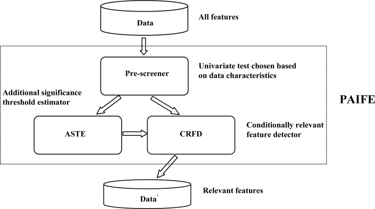
By partitioning a feature space and adaptively assessing feature-target relevancies in those subspaces, PAIFE can reliably identify subtle relationships, which otherwise are extremely difficult to detect by most feature selection methods in the presence of large numbers of features but with much fewer samples. As illustrated in Figure 1, there are two phases for irrelevant feature removal. Phase 1 is pre-screening, wherein we identify features which have direct relationships with the target that are manifested over the whole dataset. A simple univariate statistical test would be sufficient to detect these relationships. We then in phase 2 repeatedly partition the dataset into (often overlapping) subsets according to those relevant features detected by pre-screening and further identify relevant features over these partitioned subsets.

Figure 1.

Component diagram of PAIFE.

In the following subsections, we will first give definitions on feature-target relationships, followed by discussions on partitioning and conditional relationship, and how we incorporate them as the key components into our framework of PAIFE. We then discuss how data characteristics, such as sample size, number of features, and the number of multiple tests for feature-target relevancy may influence detection resolution, which is the weakest statistically significant feature-target relationship that can be found by this method. We finally describe a strategy for obtaining multiple adaptive significance thresholds in order to intelligently identify relevant features above random noise levels.

Feature-target relationships

A feature is said to be relevant to the target if there is a significant association between this feature and the target. According to their relationships with the target, we categorize features into the following three distinct groups:

• Unconditionally Relevant Features: features relevant to the target over the whole dataset;

• Conditionally Relevant Features: features relevant to the target but conditional on certain other features;

• Unconditionally Irrelevant Features: features not conditionally or unconditionally relevant to the target.

Unconditionally relevant features can be identified by a univariate test over a whole dataset. In contrast, conditionally relevant features can only be detected over certain subsets wherein such relationships manifest themselves conditional on certain other features. Features not in the first two categories fall into the category of unconditionally irrelevant features. With PAIFE, our goal is to remove the unconditionally irrelevant features to reduce the complexity of high-dimensional biomedical datasets.

Partitioning and conditional relationship

Conditional relationship refers to a concept in probability theory. In particular, two random variables X and Y are conditionally independent given a third random variable Z if the conditional probability distribution for X given Y and Z is the same as that given Z alone. That is, Prob (X = x | Y = y, Z = z) = Prob (X = x | Z = z) for any x, y, z with Prob (Z = z) > 0.

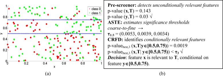
Conditional relationships are very subtle and usually extremely hard to identify. Partitioning, by dividing a domain space into a finite number of small regions, facilitates the discovery of conditional relationships since we can evaluate feature-target relationships over the partitioned subsets. Figure 2 depicts an example. Although feature x does not appear to be strongly related with the target T, by partitioning the dataset according to another feature y, PAIFE can identify a particular subset (between the dashed blue lines in Figure 2a) wherein a strong association between x and T exists. Figure 2b illustrates the step-by-step processes and results of PAIFE in identifying x and y’s relationships with T. However, when considering several thousands of features in real datasets, it is not a trivial task to effectively identify those subsets wherein meaningful feature-target associations manifest. As explained in detail later in this paper, we design PAIFE to adaptively partition a dataset and further dynamically evaluate feature-target relationships over the partitioned subsets.

Figure 2.

An example of feature-target relationships. (a) Visualization of sample data of features x, y and the target T. Horizontal and vertical axes represent features x and y, respectively. The green and red colors represent the binary classes of the target feature, T. (b) Illustration of how PAIFE works step-by-step to identify x, y’s relevancies to the target T.

While discretization methods, such as Multi-Interval Discretization10, can also be used for partitioning, they typically partition data using very coarse granularity with less control. Instead, we favor uniformly partitioning data into smaller subsets. This strategy is simple, easier to manipulate and provides control over granularity, while being computational efficient. We also adopt a coarse-to-fine strategy, starting by interrogating feature-target relationships from big and often overlapping (coarser level) subsets, and only resort to smaller (finer level) subsets when previous evaluations at the coarser level fail to reveal any significant relevancy.

Adaptive significance thresholds via artificial features

To identify the conditional relationship between a particular feature and the target, we evaluate the relevancy of this feature to the target conditional on each of the other features. This implies that the association between one feature and the target will be tested over the partitioned subsets based on each of the other features. Since there are many features and various ways of partitioning the whole dataset, we typically have to conduct thousands of tests for conditional feature-target relationships. In the presence of multiple tests, the chance of making incorrect claims of a significant (p-value ≤ 0.05) feature-target relationship is higher. Therefore, we need to define an appropriate significance threshold to avoid an inappropriately high prevalence of chance findings. The detection resolution of our method is the weakest association that can be found to be statistically significant. Larger samples and fewer multiple tests typically improve the detection resolution. Due to the fact that most genomic and proteomic datasets have thousands or more features but only a couple of hundred or fewer samples, there is often not enough power to detect the feature-target relationship conditional on two or more other features in those datasets.

We take a data-driven strategy to adaptively set up multiple significance thresholds. As previously mentioned, we evaluate feature-target relationships through multiple coarse-to-fine levels. We dynamically estimate an appropriate significance threshold at each coarse-to-fine level. In order to do so, we introduce a set of randomly generated features, which we call artificial features, similar to a concept in Tuv et al9. After pre-screening, we randomly generate a number of artificial features of the same sample size as the real features. After partitioning datasets according to those relevant features discovered during pre-screening, we test all the artificial features on their relevancies to the target over the corresponding partitioned subsets and record the lowest p-value of each artificial feature at each coarse-to-fine level and sort the corresponding p-values recorded for all the artificial features. We pick the 5^th percentile of p-values at each coarse-to-fine level as the significance threshold that we will later use to identify from the set of real features the ones relevant to the target.

Method

In this section, we describe the algorithmic and implementation details of PAIFE. PAIFE can process categorical, discrete and continuous data. In dealing with continuous data, it is important to scale data feature-wise to transform values of all the features into the same range to avoid dominance of those with larger numeric ranges. We apply a simple one-dimensional linear scaling method to scale the value of each feature. In particular, let f_max and f_min be the maximum and minimum values of feature f in a dataset. Then

$${\mathit{f}}_{\mathit{s}}=\left({\mathit{f}}_{\mathit{o}}-{\mathit{f}}_{\mathit{min}}\right)/\left({\mathit{f}}_{\mathit{max}}-{\mathit{f}}_{\mathit{min}}\right)$$

where f_o and f_s are the feature values before and after scaling, respectively. We use this scaling to map the values of each feature onto the range of [0, 1].

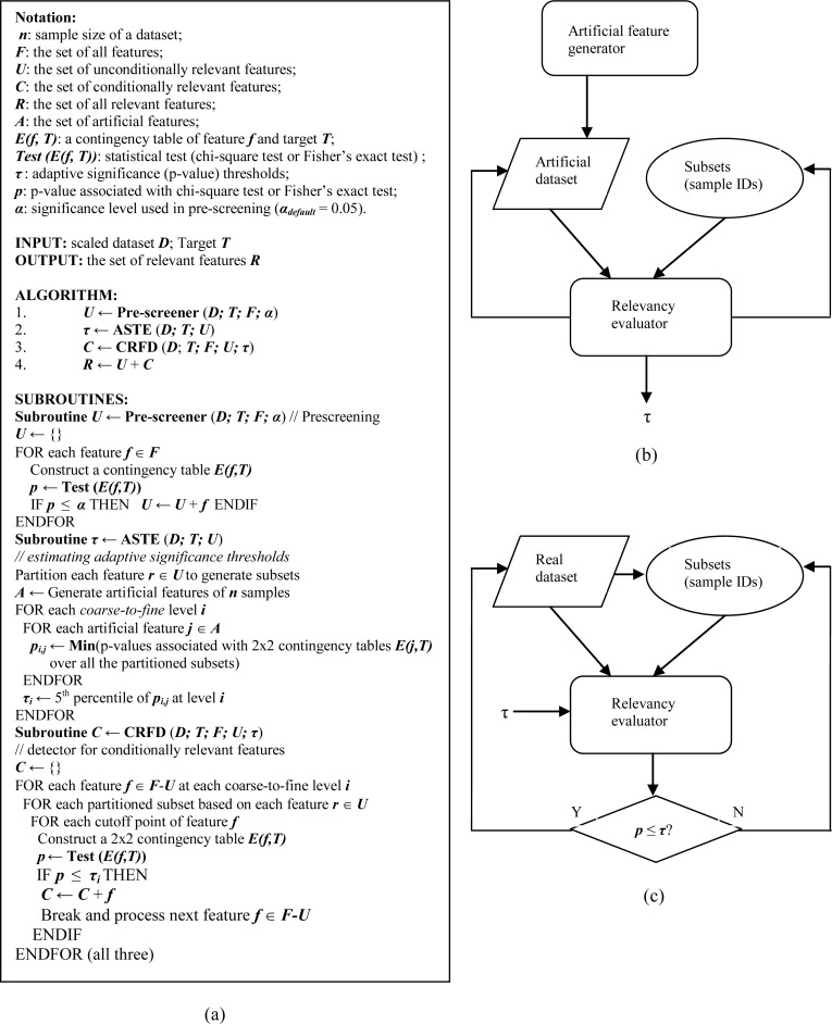
As a pre-screening process, we first identify features that are unconditionally relevant to the target by a univariate test over the whole dataset. Then according to these identified relevant features, we partition the dataset into subsets and evaluate other features’ relationships with the target over the partitioned subsets at each coarse-to-fine level. Figure 3 gives the pseudocode of algorithm PAIFE and the flowcharts of the PAIFE components: ASTE and CRFD.

Figure 3.

The algorithm of PAIFE. (a) Pseudocode; (b) the flowchart of Subroutine ASTE; (c) the flowchart of Subroutine CRFD.

Pre-screening

The goal of pre-screening is to discover all the features that are unconditionally relevant to the target typically by a univariate test, such as the chi-square test at a significance level of α = 0.05. We first divide the values of each feature into disjoint, equal-sized bins. We then discretize that feature by categorizing the feature values into the corresponding bins. After discretization, we apply the chi-square test on each feature-target contingency table. We retain all the significant features as unconditionally relevant features. At this screening stage, we chose not to apply any multiple test adjustment. Because first, there are much fewer tests involved here than in the process of evaluating conditional relationships over the partitioned datasets, the possibility of false positives is relatively low. Secondly, a larger pool of unconditionally relevant features can help capture the conditionally relevant features since more features serve as the features to be conditioned upon for partitioning. This is well in accordance with our overall conservative IFR strategy of minimizing the loss of potentially relevant features.

Univariate tests for conditional feature-target relationships

When we assess conditional feature-target relationships over the partitioned subsets, the sample size of a subset can be much smaller than that of the whole dataset. It is important to utilize appropriate univariate statistical tests to address the sample size issue for assessing the conditional feature-target relationships. We incorporated two statistical tests, namely Fisher’s exact test11 and the chi-square test12. Since Fisher’s exact test and the chi-square test are for categorical data, continuous data have to be pre-discretized for either of the tests to be applied.

Chi-square test is the most commonly used test for association between categorical variables in a form of contingency table. It has computational advantages in dealing with large and less extremely distributed datasets. However, if the counts in some cells are too small or there is a zero count, large sample approximation of chi-square distribution is no longer appropriate and the test result tends to be significant when there is no real association. Fisher’s exact test is always valid no matter how small the sample size is, but its calculation can be time-consuming.

During pre-screening, we apply the chi-square test since a whole dataset typically meets the sample size requirement imposed by chi-square test. During subsequent evaluations over partitioned subsets, we dynamically check the counts for all the cells in the corresponding contingency table. If all the cells have 5 or more samples, then we run the chi-square test; otherwise, we run Fisher’s exact test to evaluate the feature-target relationship.

Evaluating feature-target relationships over partitioned subsets

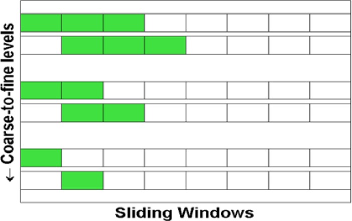
We partition the datasets according to each relevant feature identified during the pre-screening phase. We adopt a sliding window strategy to construct the subsets at each coarse-to-fine level (Figure 4). There are two parameters being involved in constructing sliding windows, one is sliding window size w; the other is step size s (s≤w), which corresponds to the window size at the finest level. Together s and w are sufficient in determining the size and overlap of the sliding windows. Assuming all the features have been scaled onto a range of [0,1], we typically set s=0.25 at each of the coarse-to-fine level while w=0.25 at the finest level and increases by 0.25 when we go one level coarser.

Figure 4.

Illustration of three-level coarse-to-fine partitioning strategy. As PAIFE moves from the coarsest (top) level to the finest level (bottom).The sliding window (green) size w decreases while the step size s remains the same.

For each partitioned subset, we adaptively apply either the chi-square test or Fisher’s exact test to identify the conditionally relevant features that are not detected in the pre-screening process. Let f be a feature under evaluation. We construct multiple 2-by-2 contingency tables of f and T using different cutoff points for f. In practice, we construct three 2-by-2 contingency tables using cutoff points 0.25, 0.50 and 0.75, respectively. We then run appropriate univariate tests on these contingency tables and compare returned p-values with the adaptive significance threshold at the same coarse-to-fine level to determine the feature’s association with the target.

Experiments

We evaluated PAIFE's performance over both synthetic and real biomedical datasets. We conducted three experiments against synthetic datasets. Experiment 1 compared PAIFE with three state-of-the-art feature selection methods in terms of absolute detection cost γ_A (being defined later). Experiments 2 and 3 evaluated PAIFE's performances with respect to changes in numbers of features and samples. We also included real-world genomic and proteomic datasets to evaluate PAIFE. We evaluated how effective PAIFE was in removing irrelevant features and how the removal of those features improved the prediction model performances.

Synthetic data

In each synthetic dataset, the target of interest was a binary variable T, 50% of samples were assigned to class 0 (T=0) and 50% to class 1 (T=1). We also generated various numbers of unconditionally and conditionally relevant features as well as random features as noise. All the features have continuous values ranging from 0 to 1, but the distribution of a particular feature depends on its relationship with the target. We numerically characterized a feature’s relevancy to the target by its classification accuracy v (0<v<1) corresponding to a particular dataset/subset.

Experiment 1

We set to compare PAIFE with some state-of-the-art feature selection/ranking methods in discovering relevant features while removing irrelevant ones. We generated a dataset including 1,000 samples of 200 features. Among all the features, 50 of them were set to be relevant to T; while the rest features were generated from a uniform distribution UNIF[0, 1], representing the noise. Among the relevant features, 10 of them were unconditionally relevant to T with v∈[0.6, 0.7]. Let set A include these 10 features and set B include the remaining 40 features that were relevant to T conditional on a feature from set A. We populated each feature x∈A as illustrated in Table 1. Specifically, we randomly chose 1,000v samples as the correctly classified cases based on feature x. If a correctly classified case was indeed in class 0 (T=0), we drew a value for x from UNIF[0, 0.5] and drew a value from UNIF(0.5, 1] if T=1. For the misclassified cases, we generated the feature values from UNIF(0.5,1] for samples in class 0 and UNIF[0,0.5] for those in class 1, respectively.

Table 1.

Illustration of feature value distribution based on classification accuracy ν.

	True Class Status
	Class 0 (T=0)	Class 1(T=1)
Correct classification	UNIF[0, 0.5]	UNIF(0.5, 1]
Incorrect classification	UNIF(0.5, 1]	UNIF[0, 0.5]

To populate values for a feature in set B, suppose that feature z∈B is associated with T conditional on feature y∈A, we randomly chose a subset with η ≤ y ≤ η + ξ, where y’s starting value η is drawn from UNIF[0, 1-0.25] and the subset range ξ = Max{0.25, UNIF[0,(1-η)/2]}. In other words, the range of y for the samples in this subset is from η to η+ξ with minimum range size of 0.25. We then generated the values of feature z for the samples in this subset in a way illustrated in Table 1, with classification accuracy v∈[0.8, 0.95]. The z values for the samples outside this subset were generated from UNIF[0,1].

We ran PAIFE at three coarse-to-fine levels with sliding window sizes of 0.25, 0.5, and 0.75, respectively. We generated 200 artificial features to adaptively estimate the significance threshold for each level of partitioning. PAIFE ranked all the features by their lowest p-values among all the tests. For comparison, we also ran three feature selection methods, namely SVM-RFE8, RELIEF4 and InfoGain13, all implemented in WEKA machine learning toolkit14, with 10-fold cross validation. All three methods returned average relevancy ranks for all the features.

We defined two metrics to measure the efficacy of a method in detecting relevant features. Suppose there are m relevant features out of totally n features. The absolute detection cost of identifying i truly relevant features, γ_A(i), is the number of features identified by a method that includes i truly relevant features. This implies that the i^th correctly identified relevant feature is ranked γ_A(i)^th by the method. Similarly, the relative detection cost, γ_R (i/m) = γ_A(i)/n, was defined as the proportion of total features needed to be detected as relevant features in order to capture a proportion of truly relevant features.

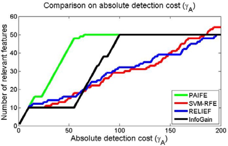
Figure 5 shows the absolute detection costs γ_A(i) of PAIFE and three other methods if we wish to detect different numbers of relevant features. We were expecting an elbow point indicating the separation between relevant and irrelevant features. The closer the elbow to the number of the truly relevant features, the higher detection power a method had. Among the four methods in comparison, all were able to identify the 10 unconditionally relevant features in set A. However, SVM-RFE and RELIEF completely failed in separating conditionally relevant features in set B from the random noise features since neither method showed any elbow at all in their γ_A curves. InfoGain indeed had the elbow point and thus, to some extent, was able to separate relevant features from noise features. However, it took about 115 features to identify all the 50 truly relevant ones. PAIFE clearly was the most effective method with an elbow at 56, which was the closest to the number (50) of truly relevant features.

Figure 5.

Comparison on absolute detection cost γ_A between PAIFE and three state-of-the-art feature selection methods: SVM-RFE8, RELIEF4 and InfoGain13.

Experiment 2

We demonstrated how well PAIFE performed against datasets of small sample sizes and varying numbers of total features and relevant features with comparisons with SVM-RFE, RELIEF and InfoGain. We fixed the sample size at 250 in all seven trials, but steadily increased the numbers of total features and relevant features up to totally 5,000 features and 2,000 relevant features from trial 1 through trial 7. The setup in trial 7 was close to the situation of real genomic datasets. We populated feature values in a way similar to experiment 1 with ν ∈[0.6, 0.7] for unconditionally relevant features and ν ∈[0.8, 0.95] for conditionally relevant features. We generated 500 artificial features to adaptively estimate the significance thresholds. To define sensitivity and specificity in the context of identifying relevant features, we refer to test positive as the case when a feature is identified as a relevant feature, and test negative as the case when a feature is claimed as an irrelevant feature by PAIFE. Thus sensitivity and specificity can be written as:

$$\begin{array}{lll}\text{Sensitivity}\hspace{0.17em}(\text{SN})\hfill & =\hfill & \frac{\#\hspace{0.17em}\text{of}\hspace{0.17em}\text{true}\hspace{0.17em}\text{positives}}{\#\hspace{0.17em}\text{of}\hspace{0.17em}\text{true}\hspace{0.17em}\text{positives}+\#\text{of}\hspace{0.17em}\text{false}\hspace{0.17em}\text{positives}}\hfill \\ \text{Specificity}\hspace{0.17em}(\text{SP})\hfill & =\hfill & \frac{\#\hspace{0.17em}\text{of}\hspace{0.17em}\text{true}\hspace{0.17em}\text{negatives}}{\#\hspace{0.17em}\text{of}\hspace{0.17em}\text{true}\hspace{0.17em}\text{negatives}+\#\text{of}\hspace{0.17em}\text{false}\hspace{0.17em}\text{negatives}}\hfill \end{array}$$

As shown in Table 2, PAIFE was robust and stable through all the trials, consistently outperformed the three compared methods in sensitivity and specificity. Furthermore, there was no significant drop in either sensitivity or specificity for PAIFE when we steadily increased the number of features through trials. In particular, in trial 7 where there were 5,000 total features, 1,000 unconditionally relevant and 1,000 conditionally relevant features, the sensitivity and specificity of PAIFE were 93.1% and 87.1%, respectively.

Table 2.

PAIFE performance against datasets of fixed sample size (250 samples) but different numbers of relevant and irrelevant features compared with SVM-RFE, RELIEF and InfoGain. #A is the number of all features; #R is the number of all relevant features; #U is the number of unconditionally relevant features; #C is the number of conditionally relevant features; #R_PAIFE is the number of features identified by PAIFE as relevant features; #TP_PAIFE is the number of correctly identified relevant features; SN (%) represents sensitivity; SP (%) stands for specificity.

Trial		1	2	3	4	5	6	7
#A		250	500	1,000	2,000	3,000	4,000	5,000
#R		100	200	400	800	1,200	1,600	2,000
#U		50	100	200	400	600	800	1,000
#C		50	100	200	400	600	800	1,000
#RPAIFE		120	242	493	907	1,391	1,776	2,248
#TPPAIFE		97	198	393	764	1,144	1,501	1,862
PAIFE	SN	97	99	98.25	95.5	95.3	93.8	93.1
	SP	84.7	85.3	83.3	88.1	86.3	88.5	87.1
SVM-RFE	SN	63.33	62.4	61.46	64.39	63.34	65.03	64.33
	SP	81.54	81.01	80.87	80.24	80.17	79.99	79.91
RELIEF	SN	62.5	62.4	60.89	63.84	62.9	64.19	63.33
	SP	80.77	81.01	80.28	79.78	79.8	79.32	78.96
InfoGain	SN	71.67	70.25	68.97	71.55	70.81	70.38	68.55
	SP	89.23	88.37	88.17	86.18	86.44	84.26	83.32

Experiment 3

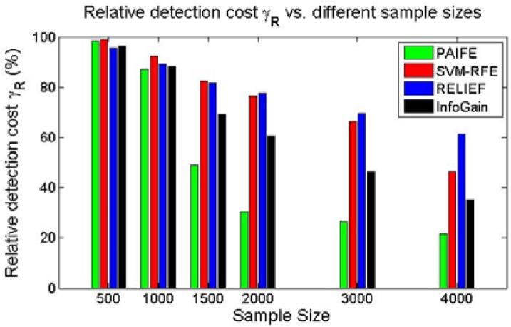
We evaluated PAIFE in identifying relevant features conditional on two other features, comparing with SVM_RFE, RELIEF and InfoGain, respectively. The setup of feature values was similar to that for experiment 1. Of totally 200 features, there were 40 relevant features (20%), among which there were 20 unconditionally relevant features and 20 conditionally relevant features. We partitioned the datasets with window size w=0.25 at the finest level and step size s=0.25. Figure 6 showed relative detection cost γ_R of the methods in comparison for identifying relevant features under different sample sizes. When sample size was not large enough (500 or lower), all four methods were powered to identify relevant features conditional on two other features. As with increasing sample size, performances of all the four methods begin to steadily improve with PAIFE consistently having the fastest pace, quickly converging to the lower bound of the relative detection cost γ_R. InfoGain came second, followed by SVM-RFE and RELIEF. Against a dataset of 4000 samples, the relative detection cost γ_R for capturing all the truly relevant features was 21.5%, approaching the theoretical lower bound of 20%, which was the ratio of the number of all truly relevant features over the number of total features. It is necessary to have sufficient number of samples in order to unambiguously identify the features that are truly associated with the target. However, methods do vary in how they are sensitive to the sample size. As we demonstrated during this experiment, although performances of all four methods improved as sample sizes increased, PAIFE converged much faster and thus needed fewer samples to achieve a reasonably high detection power than the other three methods in comparison.

Figure 6.

Relative detection cost γ_R conditional on two other features over datasets of different sample sizes.

Biomedical data

We also evaluated PAIFE over 11 genomic and 1 proteomic datasets (Table 3). For each dataset, we ran PAIFE to obtain a reduced dataset that contained only the relevant features identified by PAIFE. Then we constructed the LIBSVM classification models15 using the original full dataset and the reduced dataset respectively to evaluate their classification performance based on 10-fold cross-validation performed two times.

Table 3.

PAIFE performance over genomic (1–11) and proteomic (12) datasets.

ID	Data source	Features	Sample size		Features Removed (%)	Classification Accuracy (%)
			Class 1	Class 0		Reduced data	Full data
1	Alon et al.16	6,584	40	21	70.05	95.12	95.95
2	Beer et al.17	5,372	69	17	84.07	92.08	81.6
3	Bhattacharjee et al.18	5,372	17	52	92.68	85.71	73.1
4	Golub, et al.19	7,129	25	47	67.91	96.61	92.41
5	Hedenfalk et al.20	7,464	18	18	74.81	97.5	39.58
6	Iizuka, Oka et al.21	7,129	20	40	90.19	81.67	70
7	Pomeroy, et al.22	7,129	21	39	93.08	76.67	60.83
8	Rosenwald, et al.24	7,399	102	138	85.35	68.13	62.71
9	Singh, et al.25	12,599	52	50	46.72	64.23	57.55
10	Van’t Veer, et al.26	24,481	34	44	82.64	77.14	67.59
11	Yeoh, et al.27	12,625	48	201	90.76	87.94	80.55
12	Pusztai, et al.23	11,170	101	58	32.51	71.69	70.13

As Table 3 shows, PAIFE was in general able to remove a significant number of irrelevant features. More importantly, classification performances based on the reduced datasets either matched or improved those based on the full datasets. In average, classification accuracies across 12 datasets were improved by 14.25 percentage points.

Conclusions and future work

In this paper, we brought to attention an important problem of irrelevant feature removal that has different characteristics and goals as compared to feature selection or ranking. IFR is an important problem to study in order to avoid the risk of accidentally removing relevant features.

We proposed a novel, partitioning based adaptive method in PAIFE for irrelevant feature removal. As demonstrated in our experiments, PAIFE was robust and reliable in removing features irrelevant to the target in both synthetic and real biomedical datasets of various sample sizes, feature value distributions and feature-feature interactions. PAIFE addresses the IFR problem by adopting strategies such as coarse-to-fine level evaluations, overlapping subsets with sliding windows, and multiple adaptive significance thresholds via artificial features. We envision PAIFE to be used as an automated, data pre-processing tool for dimensionality reduction. The resulting lower-dimensional datasets would permit utilization of many readily available modeling tools.

In our future work, we plan further evaluate PAIFE with other published benchmark data, especially from genotyping studies. We would also like to investigate the feasibility of a randomization-based evaluation strategy and a more intelligent partitioning scheme to improve PAIFE’s robustness and efficacy. Furthermore, we would like to generalize our method to consider not only feature-target, but also more general feature-feature relationships.

References

- 1.Hilbe JM. 1 ed. CRC Press; 2009. Logistic Regression Models. [Google Scholar]
- 2.Edwards A. 2 ed. W H Freeman & Co (Sd); 1984. An Introduction to Linear Regression and Correlation. [Google Scholar]
- 3.Kittler J. Feature Set Search Algorithms. Pattern Recognition and Signal Processing. 1978. pp. 41–60.
- 4.Kira K, Rendell LA. Proceedings of the tenth national conference on Artificial intelligence. AAAI Press; San Jose, California: 1992. The feature selection problem: traditional methods and a new algorithm; pp. 129–134. [Google Scholar]
- 5.Kohavi R, John GH. Wrappers for feature subset selection. Artif. Intell. 1997;97(1–2):273–324. [Google Scholar]
- 6.Hall MA. Proceedings of the Seventeenth International Conference on Machine Learning. Morgan Kaufmann Publishers Inc; 2000. Correlation-based Feature Selection for Discrete and Numeric Class Machine Learning; pp. 359–366. [Google Scholar]
- 7.Breiman L. Random Forests. Mach. Learn. 2001;45(1):5–32. [Google Scholar]
- 8.Guyon I, et al. Gene Selection for Cancer Classification using Support Vector Machines. Mach. Learn. 2002;46(1–3):389–422. [Google Scholar]
- 9.Tuv E, et al. Feature Selection with Ensembles, Artificial Variables, and Redundancy Elimination. J. Mach. Learn. Res. 2009;10:1341–1366. [Google Scholar]
- 10.Fayyad, Irani Multi-Interval Discretization of Continuous-Valued Attributes for Classification Learning. 1993 [Google Scholar]
- 11.Fisher RI. Statistical methods for research workers. 14 ed. Macmillan Pub Co.; 2006. p. 362. [Google Scholar]
- 12.Plackett RL. Karl Pearson and the Chi-Squared Test. International Statistical Review / Revue Internationale de Statistique. 1983;51(1):59–72. [Google Scholar]
- 13.Mitchell TM. McGraw-Hill, Inc.; New York, NY, USA: 1997. Machine Learning; p. 432. [Google Scholar]
- 14.Witten IH. Data Management Systems. 2 ed. Morgan Kaufmann; 2005. Data Mining: Practical Machine Learning Tools and Techniques. [Google Scholar]
- 15.Chang C, Lin C. LIBSVM: A library for support vector machines. ACM Trans. Intell. Syst. Technol. 2011;2(3):1–27. [Google Scholar]
- 16.Alon U, et al. Broad patterns of gene expression revealed by clustering analysis of tumor and normal colon tissues probed by oligonucleotide arrays. Proc Natl Acad Sci U S A. 1999;96(12):6745–50. doi: 10.1073/pnas.96.12.6745. [DOI] [PMC free article] [PubMed] [Google Scholar]
- 17.Beer DG, et al. Gene-expression profiles predict survival of patients with lung adenocarcinoma. Nat Med. 2002;8(8):816–24. doi: 10.1038/nm733. [DOI] [PubMed] [Google Scholar]
- 18.Bhattacharjee A, et al. Classification of human lung carcinomas by mRNA expression profiling reveals distinct adenocarcinoma subclasses. Proc Natl Acad Sci U S A. 2001;98(24):13790–5. doi: 10.1073/pnas.191502998. [DOI] [PMC free article] [PubMed] [Google Scholar]
- 19.Golub TR, et al. Molecular classification of cancer: class discovery and class prediction by gene expression monitoring. Science. 1999;286(5439):531–7. doi: 10.1126/science.286.5439.531. [DOI] [PubMed] [Google Scholar]
- 20.Hedenfalk I, et al. Gene-expression profiles in hereditary breast cancer. N Engl J Med. 2001;344(8):539–48. doi: 10.1056/NEJM200102223440801. [DOI] [PubMed] [Google Scholar]
- 21.Iizuka N, et al. Oligonucleotide microarray for prediction of early intrahepatic recurrence of hepatocellular carcinoma after curative resection. Lancet. 2003;361(9361):923–9. doi: 10.1016/S0140-6736(03)12775-4. [DOI] [PubMed] [Google Scholar]
- 22.Pomeroy SL, et al. Prediction of central nervous system embryonal tumour outcome based on gene expression. Nature. 2002;415(6870):436–42. doi: 10.1038/415436a. [DOI] [PubMed] [Google Scholar]
- 23.Pusztai L, et al. Pharmacoproteomic analysis of prechemotherapy and postchemotherapy plasma samples from patients receiving neoadjuvant or adjuvant chemotherapy for breast carcinoma. Cancer. 2004;100(9):1814–22. doi: 10.1002/cncr.20203. [DOI] [PubMed] [Google Scholar]
- 24.Rosenwald A, et al. The use of molecular profiling to predict survival after chemotherapy for diffuse large-B-cell lymphoma. N Engl J Med. 2002;346(25):1937–47. doi: 10.1056/NEJMoa012914. [DOI] [PubMed] [Google Scholar]
- 25.Singh D, et al. Gene expression correlates of clinical prostate cancer behavior. Cancer Cell. 2002;1(2):203–9. doi: 10.1016/s1535-6108(02)00030-2. [DOI] [PubMed] [Google Scholar]
- 26.van 't Veer LJ, et al. Gene expression profiling predicts clinical outcome of breast cancer. Nature. 2002;415(6871):530–536. doi: 10.1038/415530a. [DOI] [PubMed] [Google Scholar]
- 27.Yeoh EJ, et al. Classification, subtype discovery, and prediction of outcome in pediatric acute lymphoblastic leukemia by gene expression profiling. Cancer Cell. 2002;1(2):133–43. doi: 10.1016/s1535-6108(02)00032-6. [DOI] [PubMed] [Google Scholar]