Cyber-T web server: differential analysis of high-throughput data

Abstract

The Bayesian regularization method for high-throughput differential analysis, described in Baldi and Long (A Bayesian framework for the analysis of microarray expression data: regularized t-test and statistical inferences of gene changes. Bioinformatics 2001: 17: 509-519) and implemented in the Cyber-T web server, is one of the most widely validated. Cyber-T implements a t-test using a Bayesian framework to compute a regularized variance of the measurements associated with each probe under each condition. This regularized estimate is derived by flexibly combining the empirical measurements with a prior, or background, derived from pooling measurements associated with probes in the same neighborhood. This approach flexibly addresses problems associated with low replication levels and technology biases, not only for DNA microarrays, but also for other technologies, such as protein arrays, quantitative mass spectrometry and next-generation sequencing (RNA-seq). Here we present an update to the Cyber-T web server, incorporating several useful new additions and improvements. Several preprocessing data normalization options including logarithmic and (Variance Stabilizing Normalization) VSN transforms are included. To augment two-sample t-tests, a one-way analysis of variance is implemented. Several methods for multiple tests correction, including standard frequentist methods and a probabilistic mixture model treatment, are available. Diagnostic plots allow visual assessment of the results. The web server provides comprehensive documentation and example data sets. The Cyber-T web server, with R source code and data sets, is publicly available at http://cybert.ics.uci.edu/.

INTRODUCTION

One of the most fundamental problems in bioinformatics and other sciences is the problem of differential analysis. Specifically, in its most typical bioinformatics form, this is the problem of identifying which RNA molecules, proteins, metabolites or other species behave differently between two or more different conditions or treatments, given a set of corresponding measurements. Not only is this a fundamental problem as a prerequisite for identifying the underlying driving mechanisms or deriving new diagnostic approaches, but it is also a recurrent problem both within and across different high-throughput technologies, ranging from DNA and protein microarrays, to mass spectrometry, to high-throughput sequencing in its various forms and applications (e.g. ChIP-seq, RNA-seq). While, in general, the concentrations of the molecular species within one condition are not independent of each other, during a first level of differential analysis, it is still useful to treat them as if they were independent to some extent. Furthermore, it is generally accepted that a simple fold-change approach to inference of differential behavior is not viable; rather, one must take into account the scale, i.e. the SDs, of the quantities being considered (1,2).

The Cyber-T program and web server, originally developed for DNA microarray data (3), addresses the problem of differential analysis in a way that is both flexible and efficient, using the entire set of measurements to overcome instrumental or experimental biases. The key to Cyber-T is an approach, derived from a Bayesian model, to robustly estimate the SDs, which can then be used to perform a regularized t-test.

t-test and variance regularization

More precisely, assume that, for instance, in the case of a gene X, we have a set of measurements and representing expression levels x^c and x^t, or rather their logarithms [or other normalized value (4)], in both a control and treatment situation. It is natural to assess the difference between the two groups by the difference of the means, normalized by the corresponding SD [Var(x^c − x^t)]^1/2 to yield the t statistics

(1)

Here, for each population, m = ∑_ix_i/n and s² =∑_i(x_i − m)²/(n − 1) are the well-known estimates for the mean and SD. This is exactly what a t-test does and under the proper normality assumption, it is well known that t follows approximately a Student distribution degrees of freedom, from which the corresponding P-values can be computed. While, in general, the normality assumption is reasonable for properly normalized data, it must be noted that t remains a natural statistic for ranking and assessing differences even when the normality assumptions are not perfectly satisfied, although in this case the P-values may deviate somewhat from their correct values.

The fundamental problem with the t-test for microarray or other data, however, is that the repetition numbers n_c and/or n_t are often small because experiments remain costly or tedious to repeat, even with current technologies. Small populations of size n = 1, 2 or 3 are still very common and lead to very poor estimates of the variances. Cyber-T uses a Bayesian probabilistic approach (3) to derive the following estimate of the variance in each condition, combining the empirical variance s² with a background variance :

(2)

provided ν₀ + n > 2. Here, ν₀ can be thought as a count of, pseudo-replicates with variance . The regularized variance is just a weighted average of the variances from the true and pseudo-replicates. The Student's T degrees of freedom are adjusted to account for the pseudo-replicates by simply using the total replicate count (true plus pseudo) in the well-known equation for degrees of freedom.

The background variance can be estimated by pooling all the measurements that are in a neighborhood of the measurement under consideration. While different notions of neighborhood can be introduced, Cyber-T by default ranks all the measurements by their average intensity and then uses an adjustable window around the measurement under consideration. The window neighborhood provides an empirical automated way to take into account any systematic relationship between intensity levels and their SDs, caused for instance by different technologies or instruments, without having to model this relationship explicitly.

Appropriateness for different types of data and technologies

While Cyber-T was originally developed for the analysis of DNA microarray data, the current program is applicable to any other differential analysis problem where the number of measurements is much greater than the number of experimental replicates. Since its original deployment, Cyber-T has been used extensively in the analysis of protein microarrays data (5,6) and quantitative mass spectrometry data (7).

More recently, we have begun using Cyber-T for differential analysis of RNA-Seq (8) (fragments per kilobase per million sequenced reads) FPKM values as produced by pipeline software such as cufflinks (9) or Illumina's CASAVA (in submission). While existng tools for differential analysis of RNA-Seq data use a model based on the Negative-Binomial distribution [e.g. cuffdiff (9), edgeR (10) or DESeq (11)], all of these tools use count data directly. We note that FPKM values are not discrete. Using a normal distribution approximation is reasonable in the absence of other methodologies, and to the best of our knowledge, no easy-to-use tools for differential analysis of tables of FPKM values currently exist.

Other Bayesian approaches

Although Cyber-T opportunistically mixes Bayesian and frequentist ideas by implementing a regularized t-test, a full Bayesian treatment can also be derived from the same framework. In addition, there are a number of other Bayesian approaches to differential analysis, including Efron's empirical Bayes method (12), limma (13) and BAMArray (14). There are a number of web servers implementing differential analysis tools for microarray data, e.g. as described in Morrisey and Diaz-Uriarte, 2009 (15) and references contained therein. A few of these web servers (15,16) interface to the limma R package (13). However, all of Bayesian approaches were developed after Cyber-T, and the web servers focus mainly on downstream technology-specific analysis rather than providing in-depth understanding of normalization and regularization effects. Furthermore, Cyber-T has been shown to be the most effective, or among the most effective, in many comparison studies against other Bayesian and non-Bayesian methods (17–20) especially in low-replicate regimes.

There are a couple of publicly available web server-like software packages for the differential analysis of RNA-Seq data, such as rQuant.web (21) and ExpressionPlot (22). However, facile access to these packages is limited. rQuant.web is only available as part of a larger Galaxy (23) installation. ExpressionPlot is only available for download for on-site installation. In contrast, Cyber-T is a publicly accessible web server where a user can easily upload data for analysis.

Previous Cyber-T features

As initially described (3), Cyber-T implemented the following features: limited preprocessing options including thresholding or offsetting low values and log transforms, paired and unpaired two-sample regularized t-test and a post-processing mixture model analysis of the resulting P-values. The previous web server provided only text file output. In this article, we present several new analysis features and significant improvements to the web server interface.

IMPLEMENTATION

The current version of Cyber-T is composed of a backend written in R (http://www.r-project.org/) made accessible via a web server interface. The R code requires the lattice package in addition to the vsn, multtest and geneplotter packages from Bioconductor (http://www.bioconductor.org/). The R source code and documentation are available for download. The web server interface is implemented using Django 1.3 and Python 2.7. A PostgreSQL 8.2 database is used to store results. The JavaScript JQuery library is used for interactive web features.

INPUT

Type of analysis

On the Cyber-T home page, users must select the type of experimental data to analyze. There are three basic options: (i) unpaired two conditions data; (ii) paired two conditions data and (iii) multiple conditions data. These options implement an unpaired two-sample t-test, a paired two-sample t-test and a one-way ANOVA analysis (f-test), respectively, all with the above regularization. All three of these analysis choices have similar input forms, whereby the user must upload a delimited text file and provide basic information about the layout of the data. Other parameters differ slightly by analysis type.

Preprocessing

A non-linear preprocessing step is often used with microarray and other data. A common, and previously implemented, approach is to take the natural logarithm of the data before processing. However, logarithmic transforms can have drawbacks, including being undefined for intensities less than zero, which can be generated during background subtraction by certain image quantization methods. An alternative approach called Variance Stabilizing Normalization (VSN) is based on the ‘arcsinh’ transform and an assumption of a majority of measurements being non-differentially expressed (4,24). The web server allows for preprocessing with optional low-value thresholding or offsetting and optional logarithmic or VSN normalizations. If a logarithmic or VSN is chosen, plots displaying the effect of normalization are generated (Figures 2 and 3).

Figure 2.

Plasmodium falciparum mean raw intensity versus empirical SD showing a clear mean–variance dependence. Outliers have been removed to make the relationship clearer.

Figure 3.

Plasmodium falciparum VSN mean normalized intensity versus empirical and Bayes-regularized SD. The systematic mean–variance relationship seen in the raw data has largely been removed in the empirical variance. The regularization shows regression toward the mean experiment SD.

Bayesian-regularization parameters

The user is asked to provide a window size and a confidence parameter for the Bayesian regularization. The window size determines how the estimate of the background variance is calculated. By default, the window size is set to 101 genes (50 on each side, except for boundary effects), though with an extremely low (<100) or extremely large (>50 000) number of measurements, this size should be reduced or increased, respectively. Cyber-T computes the background variance by pooling the variances of the genes in a neighborhood determined by the window size and the mean value associated with the gene under consideration.

The confidence parameter corresponds to the background pseudo-counts (ν₀) from Equation (2). A reasonable rule of thumb is to set the confidence such that the total number of replicates (biological replicates plus pseudo-counts, or n + ν₀) is = 8. For example, in a paired analysis where n = 3, the confidence parameter can be set to 5. There are two extreme confidence regimes that are handled by Cyber-T. If the confidence is left blank or is set to 0, then Cyber-T assumes no background and a standard t-test or ANOVA is performed with no regularization. At the other extreme, when the confidence is set to infinity (which is the default in the case of a single observation with n = 1), then the overall variance estimates are completely determined by the prior using the values in the sliding window, corresponding to pure regularization. Both extremes are allowed, but the user is provided with a warning. If a user inputs data with a single replicate and a confidence of 0, a default confidence of 5 is chosen to perform the Bayes-regularized analysis and the user is provided a warning.

Figure 1 shows an illustrative plot of how Bayes-regularized variance estimates can alleviate low-replicate issues.

Figure 1.

Mean versus SD plots for Condition 1 of both the low- and high-replicate Plasmodium falciparum protein microarray data sets. The Bayes-regularized estimates approximate the ‘truth’ of the high-replicate empirical measurements better than the low-replicate empirical measurements. The plots are shown with density estimate smoothing, a plotting option on the web server. Darker colors indicate high local density.

Post-processing

Multiple tests correction

High-throughput analyses in bioinformatics can involve tens of thousands of simultaneous hypothesis tests, or more. In such large multiplicity regimes, naive test statistic interpretations lead to large numbers of Type I errors (false positives) (25). In broad terms, there are two common approaches to alleviate these problems: (i) a probabilistic mixture model approach; or (ii) a frequentist correction of the P-values to control Type I errors. Both approaches are implemented in Cyber-T.

For the first approach, the t-test of Equation (1) with the Bayes-regularized SDs of Equation (3) provides for each measurement a P-value. The distribution of these P-values can typically be modeled as a mixture of 2 β- distributions, a flat distribution for the background associated with the majority of non-differential measurements, and a peaked distribution close to 0 for the differential measurements. From this mixture model, one can derive: estimates of true/false positive rates at all thresholds; estimates of true/false negative rates at all thresholds; (Receiver Operating Characteristic) ROC curves; and (Posterior Probabilities of Differential Expression) PPDEs (26,27). Frequentist P-value corrections either use the Bonferroni or Benjamini & Hochberg corrections. The Bonferroni method provides a stringent control of the Type I errors, but at the expense of a possibly large number of Type II errors (false negatives). The Benjamini & Hochberg method provides much less strict control of Type I errors, but with complementary less Type II errors. Cyber-T provides the user with the results obtained with all three methods.

Pairwise post-hoc tests

Low P-values in a one-way ANOVA are indicative only of a difference across all groups. Post-processing options are available to help determine which particular groups or comparisons are different. Pairwise posthoc tests using the regularized variance estimates and either Tukey's Honestly Significant Difference or Scheffe's method (28) are available. We note that the P-values from the pairwise post-hoc tests are ‘not’ corrected for multiple-testing. This is done to provide flexibility to the user. Post hoc P-values should only be examined for measurements that are significant at an acceptable multiple test corrected omnibus ANOVA P-value.

OUTPUT

The initial results page presents a table of the top 25 measurements ranked by P-value. This table contains normalized values and all calculated statistics including variance estimates, t statistics, and P-values. Depending on the options chosen earlier, posterior probabilities of differential expression, multiple tests corrections, and P-values from pairwise post hoc tests are given. Complete results are available as a formatted table or, through a link, as a downloadable text file. If the PPDE analysis is selected, the mixture coefficients of the models are also reported. These values provide information about the overall occurrence of differential and non-differential measurements in the data set.

Plotting

Cyber-T generates several plots to help users assess their data, depending on the options chosen. These include: scatterplots of the raw and normalized data, variance versus mean plots for raw and normalized data, variance versus mean plots for empirical variance and Bayes-regularized variance, effect of regularization plots and ROC plots. By examining these output plots, the user can identify data irregularites as well as visualize and understand the effects of normalization and regularization in the analysis (Figures 2–4).

Figure 4.

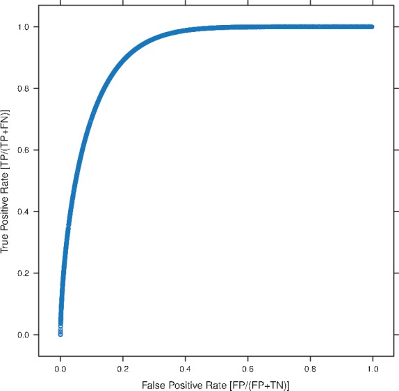
Plasmodium falciparum ROC curve from PPDE analysis. ∼25% false positives must be accepted to discover ∼90% of the true positives.

Two options for plotting are available. The first is the use of a smoothed color density representation in all scatterplots. This is implemented using utilities from the geneplotter R package. Kernel density estimates are made for the x- and y-axes and data is binned into a large grid. Then a smoothed map of these densities is plotted where dark colors represent regions of high density. This allows the user to visualize the 2D distribution of the data and identify important relationships. The second available option is outlier removal. Here datapoints more than two inter-quartile ranges above or below the first or third quartile, respectively, are removed. By choosing this option, the user may be able to identify relationships in the data that are obscured from the much lower resolution needed to plot all the data. Both plotting options are turned on by default.

EXAMPLE DATA SETS

To assist users in working with Cyber-T, several example data sets are provided along with buttons to load all the necessary parameters for their analysis. Each analysis page has a section at the top with links to use an example data set, as well as links to help sections providing additional details. At least one example data set is provided for each of the discussed high-throughput technologies, including an RNA-Seq data set of gene level FPKM values from the ENCODE project (29).

Here, we walk through the analysis of one example data set, a previously published humoral immune response protein microarray study (6). The technology is thoroughly described in the study manuscript, but briefly it measures antibody response to individual peptides on an array in a manner similar to an ELISA. The data come from a prospective study of the humoral immune response to Plasmodium falciparum in children from Kambila, Mali. The protein microarray contains 2320 P. falciparum proteins spotted on the array. The study used an unpaired two sample t-test, where the groups are sera samples from children who did (n = 29) and did not (n = 12) have clinical episodes in the following malaria season.

To exhibit Cyber-T effectiveness in low-replication regimes, we present plots from a randomly drawn subset of this data with only two replicates in each condition. A plot showing how Cyber-T regularizes the variance estimates from the low-replicate data toward the high-replicate empirical estimates are shown in Figure 1. Details of both the high- and low-replicate data sets are available on the web server, as ‘Complete P. falciparum Protein Microarray Data and Low-replicate P. falciparum Protein Microarray Data’ respectively, under ‘Example Data sets’ on the ‘Unpaired Two Conditions’ Data page. Clicking on the available links on this page will load the data and all parameters necessary for the recommended analysis.

The web server generates several diagnostic plots during the low-replicate data analysis. A few of the plots generated using the low-replicate humoral immune response data are shown here. Figure 2 shows a mean–variance plot of the raw unnormalized data and empirical SDs (with outliers removed). Figure 3 shows similar plots with VSN normalized data and both empirical and Bayes-regularized SD. By comparision, the user can see the effects of normalization: the raw data has a systematic mean–variance dependence, which is removed by normalization. Figure 3 also allows the user to visually assess the effect of regularization. Here, the empirical SDs are squashed towards the mean. Finally, Figure 4 shows the ROC plot for the analysis constructed using the PPDE analysis, allowing the user to quickly see the tradeoffs between false negatives and false positives.

CONCLUSION

The Cyber-T program and web server provides an easy to use and validated tool for differential analysis of high-throughput data. The basic idea is to use a sliding window to define a neighborhood from which to derive a more robust estimate of the SD of each measurement. Several pre-processing and postprocessing options are available to refine the analysis. Result tables and plots for interpretation are presented in a user-friendly manner.

FUNDING

National Institutes of Health (NIH) [LM010235-01A1 and 5T15LM007743 to P.B.]. Funding for open access charge: NIH [5T15LM007743].

Conflict of interest statement. None declared.

REFERENCES

- 1.Allison DB, Cui X, Page GP, Sabripour M. Microarray data analysis: from disarray to consolidation and consensus. Nat. Rev. Genet. 2006;7:55–65. doi: 10.1038/nrg1749. [DOI] [PubMed] [Google Scholar]
- 2.Miron M, Nadon R. Inferential literacy for experimental high-throughput biology. Trends Genet. 2006;22:84–89. doi: 10.1016/j.tig.2005.12.001. [DOI] [PubMed] [Google Scholar]
- 3.Baldi P, Long AD. A Bayesian framework for the analysis of microarray expression data: regularized t-test and statistical inferences of gene changes. Bioinformatics. 2001;17:509–519. doi: 10.1093/bioinformatics/17.6.509. [DOI] [PubMed] [Google Scholar]
- 4.Huber W, von Heydebreck A, Sültmann H, Poustka A, Vingron M. Variance stabilization applied to microarray data calibration and to the quantification of differential expression. Bioinformatics. 2002;18(Suppl. 1):96–104. doi: 10.1093/bioinformatics/18.suppl_1.s96. [DOI] [PubMed] [Google Scholar]
- 5.Sundaresh S, Doolan DL, Hirst S, Mu Y, Unal B, Davies DH, Felgner PL, Baldi P. Identification of humoral immune responses in protein microarrays using DNA microarray data analysis techniques. Bioinformatics. 2006;22:1760–1766. doi: 10.1093/bioinformatics/btl162. [DOI] [PubMed] [Google Scholar]
- 6.Crompton PD, Kayala MA, Traore B, Kayentao K, Ongoiba A, Weiss GE, Molina DR, Burk C, Waisberg M, Jasinskas A, et al. A prospective analysis of the Ab response to Plasmodium falciparum before and after a malaria season by protein microarray. Proc. Natl Acad. Sci. USA. 2010;107:6958–6963. doi: 10.1073/pnas.1001323107. [DOI] [PMC free article] [PubMed] [Google Scholar]
- 7.Kaake RM, Wang X, Huang L. Profiling of protein interaction networks of protein complexes using affinity purification and quantitative mass spectrometry. Mol. Cell Proteomics. 2010;9:1650–1665. doi: 10.1074/mcp.R110.000265. [DOI] [PMC free article] [PubMed] [Google Scholar]
- 8.Parkhomchuk D, Borodina T, Amstislavskiy V, Banaru M, Hallen L, Krobitsch S, Lehrach H, Soldatov A. Transcriptome analysis by strand-specific sequencing of complementary DNA. Nucleic Acids Res. 2009;37:e123. doi: 10.1093/nar/gkp596. [DOI] [PMC free article] [PubMed] [Google Scholar]
- 9.Trapnell C, Williams B, Pertea G, Mortazavi A, Kwan G, van Baren MJ, Salzberg SL, Wold BJ, Pachter L. Transcript assembly and quantification by RNA-Seq reveals unannotated transcripts and isoform switching during cell differentiation. Nat. Biotechnol. 2010;28:511–515. doi: 10.1038/nbt.1621. [DOI] [PMC free article] [PubMed] [Google Scholar]
- 10.Robinson MD, McCarthy DJ, Smyth GK. edgeR: a Bioconductor package for differential expression analysis of digital gene expression data. Bioinformatics. 2010;26:139–140. doi: 10.1093/bioinformatics/btp616. [DOI] [PMC free article] [PubMed] [Google Scholar]
- 11.Anders S, Huber W. Differential expression analysis for sequence count data. Genome Biol. 2010;11:R106. doi: 10.1186/gb-2010-11-10-r106. [DOI] [PMC free article] [PubMed] [Google Scholar]
- 12.Efron B, Tibshirani R, Storey J, Tusher V. Empirical Bayes analysis of a microarray experiment. J. Am. Stat. Assoc. 2001;96:1151–1160. [Google Scholar]
- 13.Smyth GK. Linear models and empirical Bayes methods for assessing differential expression in microarray experiments. Stats. Appl. Genet. Mol. Biol. 2004;3 doi: 10.2202/1544-6115.1027. [DOI] [PubMed] [Google Scholar]
- 14.Ishwaran H, Rao JS, Kogalur UB. BAMarraytrade mark: Java software for Bayesian analysis of variance for microarray data. BMC Bioinformatics. 2006;7:59. doi: 10.1186/1471-2105-7-59. [DOI] [PMC free article] [PubMed] [Google Scholar]
- 15.Morrissey ER, Diaz-Uriarte R. Pomelo II: finding differentially expressed genes. Nucleic Acids Res. 2009;37:W581–W586. doi: 10.1093/nar/gkp366. [DOI] [PMC free article] [PubMed] [Google Scholar]
- 16.Rainer J, Sanchez-Cabo F, Stocker G, Sturn A, Trajanoski Z. CARMAweb: comprehensive R- and bioconductor-based web service for microarray data analysis. Nucleic Acids Res. 2006;34:W498–W503. doi: 10.1093/nar/gkl038. [DOI] [PMC free article] [PubMed] [Google Scholar]
- 17.Choe SE, Boutros M, Michelson AM, Church GM, Halfon MS. Preferred analysis methods for Affymetrix GeneChips revealed by a wholly defined control dataset. Genome Biol. 2005;6:R16. doi: 10.1186/gb-2005-6-2-r16. [DOI] [PMC free article] [PubMed] [Google Scholar]
- 18.Murie C, Woody O, Lee AY, Nadon R. Comparison of small n statistical tests of differential expression applied to microarrays. BMC Bioinformatics. 2009;10:45. doi: 10.1186/1471-2105-10-45. [DOI] [PMC free article] [PubMed] [Google Scholar]
- 19.Dondrup M, Hüser AT, Mertens D, Goesmann A. An evaluation framework for statistical tests on microarray data. J. Biotechnol. 2009;140:18–26. doi: 10.1016/j.jbiotec.2009.01.009. [DOI] [PubMed] [Google Scholar]
- 20.Zhu Q, Miecznikowski JC, Halfon MS. Preferred analysis methods for Affymetrix GeneChips. II. An expanded, balanced, wholly-defined spike-in dataset. BMC Bioinformatics. 2010;11:285. doi: 10.1186/1471-2105-11-285. [DOI] [PMC free article] [PubMed] [Google Scholar]
- 21.Bohnert R, Rätsch G. rQuant.web: a tool for RNA-Seq-based transcript quantitation. Nucleic Acids Res. 2010;38:W348–W351. doi: 10.1093/nar/gkq448. [DOI] [PMC free article] [PubMed] [Google Scholar]
- 22.Friedman BA, Maniatis T. ExpressionPlot: a web-based framework for analysis of RNA-Seq and microarray gene expression data. Genome Biol. 2011;12:R69. doi: 10.1186/gb-2011-12-7-r69. [DOI] [PMC free article] [PubMed] [Google Scholar]
- 23.Goecks J, Nekrutenko A, Taylor J. Galaxy: a comprehensive approach for supporting accessible, reproducible, and transparent computational research in the life sciences. Genome Biol. 2010;11:R86. doi: 10.1186/gb-2010-11-8-r86. [DOI] [PMC free article] [PubMed] [Google Scholar]
- 24.Rocke DM, Durbin B. Approximate variance-stabilizing transformations for gene-expression microarray data. Bioinformatics. 2003;19:966–972. doi: 10.1093/bioinformatics/btg107. [DOI] [PubMed] [Google Scholar]
- 25.Dudoit S, Shaffer JP, Boldrick JC. Multiple hypothesis testing in microarray experiments. Stat. Sci. 2003;18:71–103. [Google Scholar]
- 26.Allison DB, Gadbury GL, Heo M, Fernandez JR, Lee C-K, Prolla TA, Weindruch R. A mixture model approach for the analysis of microarray gene expression data. Comput. Stat. Data Anol. 2002;39:1–20. [Google Scholar]
- 27.Hung SP, Baldi P, Hatfield GW. Global Gene Expression Profiling in Escherichia coli K12. The effects of leucine-responsive regulatory protein. J. Biol. Chem. 2002;277:40309–40323. doi: 10.1074/jbc.M204044200. [DOI] [PubMed] [Google Scholar]
- 28.Scheffé H. The Analysis of Variance. New York, NY: Wiley; 1959. pp. 66–77. [Google Scholar]
- 29. The ENCODE (ENCyclopedia Of DNA Elements) Project. (2004) Science306, 636–640. [DOI] [PubMed] [Google Scholar]