Accurate detection of outliers and subpopulations with Pmetrics, a non-parametric and parametric pharmacometric modeling and simulation package for R

Abstract

Introduction

Non-parametric population modeling algorithms have a theoretical superiority over parametric methods to detect pharmacokinetic and pharmacodynamic sub-groups and outliers within a study population.

Methods

The authors created “Pmetrics”, a new Windows and Unix R software package that updates the older MM-USCPACK software for non-parametric and parametric population modeling and simulation of pharmacokinetic and pharmacodynamic systems. The parametric iterative two-stage Bayesian (IT2B) and the non-parametric adaptive grid (NPAG) approaches in Pmetrics were used to fit a simulated population with bimodal elimination (Kel) and unimodal volume of distribution (Vd), plus an extreme outlier, for a one-compartment model of an intravenous drug.

Results

The true means (SD) for Kel and Vd in the population sample were 0.19 (0.17) and 102 (22.3), respectively. Those found by NPAG were 0.19 (0.16) and 104 (22.6). IT2B estimated them to be 0.18 (0.16) and 104 (24.4). However, given the bimodality of Kel, no subject had a value near the mean for the population. Only NPAG was able to accurately detect the bimodal distribution for Kel and to find the outlier in both the population model and in the Bayesian posterior parameter estimates.

Conclusion

Built on over three decades of work, Pmetrics contains a robust, reliable, and mature non-parametric approach to population modeling, which was better than the parametric method at discovering true pharmacokinetic sub-groups and an outlier.

Introduction

Pharmacometrics, the discipline incoporating pharmacokinetic and pharmacodynamic modeling and simulation, has revolutionized the drug development process and has the potential to revolutionize individual patient care through clinical application.^1–3 For over 35 years, our Laboratory of Applied Pharmacokinetics (LAPK) at the University of Southern California (USC) in Los Angeles, California has developed and released pharmacometric software. While we have an ITerative 2-stage Bayesian (IT2B) parametric method, for many years our focus has been on non-parametric methods. We started with the Non-Parametric Expectation Maximization (NPEM) algorithm,⁴ and moved to a combination of NPEM for the first cycle of the model fitting process, followed by cycles that use our Non-Parametric Adaptive Grid (NPAG) algorithm of Leary and Burke (described by Baek⁵ and Bustad et al,⁶ with a definitive description now submitted elsewhere for publication by Yamada et al).

We have focused on non-parametric pharmacometric methods because of some desirable properties not present in commonly used parametric methods. Non-parametric algorithms do not approximate the likelihood function, as do parametric algorithms that are not based on maximum likelihood, e.g. FO, FOCE, FOCEI. An exact likelihood function makes non-parametric methods statistically consistent.^7,8 In other words, for a given model, convergence upon true population parameter value distributions is assured as sample size increases, which is not true for approximated functions. Non-parametric methods also make no assumptions about the underlying distribution of parameter values in the population, which theoretically makes them superior to all parametric methods for detecting unexpected sub-populations or outliers. Finally, the discrete nature of non-parametric population models naturally lends itself to multiple-model optimal control, a technique that achieves target concentrations in individual patients with maximum precision,³ and has its origins in flight control algorithms employed by the aerospace industry.^9,10

Over the years, our laboratory’s pharmacometric algorithms have been implemented in DOS-based software (USC*PACK) and, later, Windows software with a graphical interface (MM-USCPACK). While the Windows software was perhaps easier to use through familiar point-and-click methods, it was hampered in several ways. The formats of the input and output files were unique to MM-USCPACK, making it difficult for researchers to use who were familiar with other packages. Graphing was rudimentary and limited to a few standard plots, and there was no easy way to analyze MM-USCPACK output with standard statistical or even spreadsheet software.

Therefore, for this manuscript, we had two aims. The first was to describe “Pmetrics” (short for pharmacometrics), our newly available package for the statistical and graphing platform R¹¹ that incorporates all of our algorithms and methods with numerous enhancements, making them available in a very powerful, integrated, and flexible way to the research community. Our second aim was to test the theoretical advantage of the non-parametric approach to accurately characterize subpopulations and outliers by estimating population and individual pharmacokinetic parameters in a simulated dataset with the parametric IT2B and non-parametric NPAG algorithms in Pmetrics.

Materials and Methods

Overall strategy

In Pmetrics, we integrated R with the three existing LAPK software components: NPAG, IT2B and a Monte Carlo Simulator, which are written in Fortran. Thus both R and a Fortran compiler are necessary to run Pmetrics. R is free and can be downloaded from the internet (http://www.r-project.org). We suggest the freely available gfortran compiler and describe where to obtain the proper version on our website and in the User’s Manual.¹²

NPAG will create a non-parametric population mixed-effects model consisting of discrete support points, each point having a set of estimates for all parameters in the model plus an associated probability (weight) of that set of estimates. There can be at most one point for each subject in the study population. Random effects are the values of the model parameters (e.g. clearance) in the population. The fixed effect is the error model, consisting of a polynomial to describe assay variance (error), and gamma, a multiplier of assay variance, or lambda, an addend to assay variance, each estimated as a single value in the population. There is no need to make any assumptions about the underlying distribution of random effects (i.e., model parameter values), such as Gaussian. IT2B is generally used to estimate initial ranges of parameter values to pass to NPAG, under the assumption that the underlying distributions of those values are normal or transformed to normal. The Simulator is a general purpose Monte Carlo simulator, which samples new sets of parameter values from prior parametric or non-parametric distributions for any pharmacokinetic/pharmacodynamic model. From each sampled set of parameter values, the Simulator will calculate observations based on a template of inputs, covariates, and output measurement times.

R is compiled line by line, and this compromise in speed would have prolonged model fitting run times considerably. Furthermore, the three components above contain over 25,000 lines of Fortran code, and we did not have the resources to rework this natively in R. Therefore, early in the process, we decided to embed the Fortran engines within R.

R has functions to enable passage of objects to and from Fortran processes executed within R, but they are rudimentary and were not flexible enough for our purposes. Furthermore, we did not want to “tie up” R while NPAG or IT2B were cycling, thereby preventing other work with R. Therefore, we decided to use R to write operating system (OS)-specific batch files that would provide the necessary input to run NPAG and IT2B, executing them as separate processes (i.e. in a Unix or DOS terminal window), and then automatically extracting the outputs. This extraction makes the results of the run available for post-processing by R, with access to all of its statistical and plotting functions. In contrast, the Simulator is run as a compiled Fortran executable entirely within an OS shell embedded in R, since simulations typically are completed in minutes.

Enhancing existing software

We made numerous enhancements to NPAG, IT2B and the Simulator. We drastically changed and standardized the structure of the subject data input files to be the same across all three components and to be very similar in format to that of other modeling packages. Our motivation was to make it as simple as possible for researchers to use Pmetrics without having to completely re-format existing datasets and risk data corruption. Input to Pmetrics is now a text file that can either be comma or semi-colon delimited. Support is recognized for period and comma decimal separators. These files can be edited in R, any text editor, or various spreadsheet programs (e.g. Excel). The overall format is one event per row, with familiar column headings such as ID, TIME and EVID for subject identifier, relative time in decimal hours, and event identifier, respectively. There is support for ADDL (additional) dosing and SS (steady state dosing), the latter using a novel algorithm, which we will publish separately, designed to efficiently calculate steady-state conditions for even the most complex non-linear model described by ordinary differential equations. Covariates are specified as columns in the data file, and users are given the option to extrapolate between covariate row entries for a given subject as piecewise constant or linear functions. Further details of the data file format are available in the Pmetrics User’s Manual.¹²

We modified the Fortran code of each component to run under Unix as well, making the package available to Macintosh users in addition to Windows users, since R is platform independent. The code contains numerous branches that depend on automatic detection of the user’s operating system (OS). There is only one version of the Fortran source code, which runs under both platforms and makes maintenance easier, although Pmetrics is distributed in OS-specific versions because the Fortran code is partially compiled.

We have also made several enhancements to the operation of NPAG and IT2B, increasing their speed and flexibility tremendously for many models. These changes are in the structural model file format, and the engine code itself. The model file is Fortran code, and several examples in a model library are available from our website (www.lapk.org). Even someone who is not familiar with Fortran coding can easily modify them.

What are these operational enhancements? Unlike previous versions of the software, up to seven inputs (e.g. combinations of drugs) and six outputs may now be modeled simultaneously. In addition to its pharmacokinetic parameters, each drug may have its own bioavailability, lag time, and initial conditions. These three parameter types, which are handled outside differential or analytic equations, can be omitted or specified as simple random variables to be estimated or as more complex equations that can include conditional statements or covariate relationships. For example, one can model three formulations of a drug simultaneously and independently fit bioavailability parameters for two, relative to the first, depending on the value of the formulation covariate. Initial conditions for a compartment can be specified as a variable to be fitted, or any equation with or without covariates, e.g. equal to a measured pre-dose concentration multiplied by the current iteration’s estimate of volume for that compartment.

For single drugs, many models that previously required differential equations to solve can now be solved analytically, thus converging approximately 10,000 times faster. Any model that can be reduced to a one- to three- compartment model with linear input and rate transfer constants can be solved analytically. This includes models with lag times, bioavailability parameters, initial conditions, conditional parameters and complex covariate models.

We have written new output routines for NPAG and IT2B to generate files specifically designed for easy importation into R. Although these files are text based like the older output files (which are still provided), they are largely free of comments, headers, and spacing that are helpful to humans, but not computers.

We have expanded our Simulator’s capabilities too. In Pmetrics, users can automatically simulate using a prior distribution from NPAG or IT2B. For the non-parametric distribution from NPAG, one can either simulate from the means and covariance matrix of the entire joint density, or can use each individual population model support point as the mean of a normal distribution within a larger, multimodal, multi-variate distribution, with each mode weighted according to the probability of the point. In this semi-parametric simulation, the covariance matrix is evenly divided across all the modes, as in the method of Goutelle et al.¹³ Of course, users may manually specify any prior they wish, without previously running either NPAG or IT2B. In all cases, the user has the option to truncate simulated parameter values to reasonable physiologic ranges. In this case, the simulator will report the means and covariances for the entire simulated population, the number of simulated sets discarded for exceeding boundaries, and the means and covariances of the final, retained set.

The Simulator uses the same data files and model files as for population analyses by NPAG and IT2B. One can specify which subjects in the data file are to be used as dosing/sampling/covariate templates for simulation of new sets of model parameter values and associated time-output profiles, making numerical and visual predictive checks for internal model validation easy. For example, in Pmetrics we have included functions to use the Simulator for automatic plotting of prediction discrepancies (pd) – also termed standardized visual predictive checks – after NPAG runs.^14,15

Finally, we have worked hard to thoroughly document Pmetrics. A comprehensive User’s Manual is available for download in .pdf format from our website¹² and all Pmetrics functions are fully documented with help files in R. Video tutorials, sample datasets, R scripts, and model files to run Pmetrics are also available from our website, as is a discussion forum. We are frequently adding new capabilities to Pmetrics (and fixing bugs!) that we and other users desire. The package will automatically notify users who have an internet connection with a brief message upon launching in R when a new version is available.

Writing R code

We began Pmetrics as a series of R functions to process outputs from NPAG and IT2B runs. Over time, the code evolved into a self-contained package that meets all standards described in the manual on “Writing R Extensions”, available at http://cran.r-project.org/ and following the “Manuals” link on the sidebar. We used the “devtools” package¹⁶ to assist with documentation for R help files and building the Pmetrics package into binaries for installation into R.

Pmetrics command overview

Pmetrics has groups of R commands or functions named logically to run each of the Fortran components and to extract the output. These are extensively documented within R by using the help(command) or ?command syntax.

• NPAG functions: NPrun, NPparse, NPload, NPreport

• IT2B functions: ITrun, ITparse, ITload, ITreport, ERRrun

• Simulator functions: SIMrun, SIMparse

For IT2B and NPAG, the “run” functions generate batch files, which when executed, launch the software programs to do the analyses. ERRrun is a special implementation of IT2B designed to estimate the assay error polynomial coefficients from the data when they cannot be calculated from assay validation data supplied by the analytical laboratory. These coefficients (C0, C1, C2, C3) are used to calculate the standard deviation (error) of each observation for appropriate weighting in the fitting process, using the equation: SD = C0 + C1*[obs] + C2*[obs]² + C3*[obs]³, where [obs] is the observation.

The batch files contain all the information necessary to complete a run, tidy the output into a date/time stamped directory with meaningful subdirectories, extract the information, generate a report, and make a saved Rdata file of parsed output which can be quickly and easily loaded into R. On Mac (Unix) systems, the batch file will automatically launch in a Terminal window. On Windows systems, the batch file must be launched manually. In both cases, the execution of the program to do the actual model parameter estimation is independent of R, so that the user is free to use R for other purposes. For the Simulator, the “run” function will execute the program directly within R.

For all programs, the “parse” functions will extract the primary output from the program into meaningful R data objects. For NPAG and IT2B, this is done automatically at the end of a successful run, and the objects are saved in the output subdirectory as NPAGout.Rdata or IT2Bout.Rdata, respectively.

For IT2B and NPAG, the “load” functions can be used to load the above Rdata files after a successful run. The “report” functions are automatically run at the end of a successful run, and these will generate an HTML page with summaries of the run, as well as the .Rdata files and other objects. The default browser will be automatically launched for viewing of the HTML report page.

Within Pmetrics there are also functions to manipulate data files and process and plot extracted data. These are summarized in Table 1, and again, all functions have extensive help files and examples that can be examined in R by using the help(command) or ?command syntax.

Table 1.

The most common Pmetrics functions used to manipulate data before and after running NPAG, IT2B, or the Simulator

Pmetrics function	Comment
Manipulate data files
PMreadMatrix	Read a Pmetrics data file into R
PMcheckMatrix	Check an R data frame for errors which would cause a run to fail
PMwriteMatrix	Write an R data frame to a new Pmetrics data file
Process data
makeAUC	Calculate AUC over any time interval from a variety of inputs using the trapezoidal approximation
makeCov†	Make a data frame (class PMcov*) containing Bayesian posterior parameter estimates for each subject with their mean covariate values, suitable for covariate analysis with linear or non- linear regression for example
makeCycle†	Make a list (class PMcycle*) containing cycle values for log-likelihood, Akaike and Bayesian Information Criteria, gamma/lambda (fixed-effect process noise multiplier of assay error), mean/median/SD values for each random model parameter normalized to the cycle 1 value, all to assist with assessment of convergence
makeFinal†	A list (class PMfinal*) with summary statistics for the final cycle parameter estimates (e.g. mean, median, covariance, etc.) after an NPAG or IT2B run, additionally with the non-parametric joint density after an NPAG run
makeNCA	Run a non-compartmental analysis on the full, predicted, first-dose profiles from an NPAG run (see makePost). This will calculate AUC by the trapezoidal rule from time 0 to the time of the next dose (or all time points for a single-dose study) and AUMC over the same interval. Extrapolation to infinity of AUC and AUMC, using the last 6 predictions in the interval is made, along with reporting of clearance, maximum concentration, time to maximum, and half-life.
makeOP†	A data frame (class PMop*) with subject identifiers, times, observations, predictions (based on population or individual posterior parameter distributions) and errors, all suitable for observed vs. predicted and residual plots
makePost†	Create predictions for each subject and output at user-specified intervals using the mean, median, or mode of individual Bayesian posterior parameter distributions
Plot Pmetrics objects*
plot.PMcov	The relationship between any two columns (i.e. Bayesian posterior parameters and covariates) of a PMcov object.
plot.PMcycle	The data in a PMcycle object vs. cycle number
plot.PMfinal	Univariate or bivariate marginal final cycle parameter value distributions in a PMfinal object
plot.PMmatrix	Raw time-observation data from a data file read by the PMreadMatrix command, with a variety of options, including joining observations with line segments, including doses, overlaying plots for all subjects or separating them, including individual posterior predictions, color coding according to groups and more
plot.PMop	Observed vs. population or individual Bayesian posterior predicted data or residual plots (see below).
plot.PMsim	Simulated time-concentration profiles from Simulator output via SIMparse, overlaid as individual curves or summarized by customizable quantiles (e.g. 5th, 25th, 50th, 75th and 95th percentiles); inclusion of observations in a population can be used to return a visual and numerical predictive check
plot.PMdiag	Generates a prediction discrepancy (pd) normal quantile-quantile (Q-Q) plot, pd histogram, pd vs. time plot, and a pd vs. prediction plot to visualize results of simulation-based internal model diagnostics accessed with the PMdiag command
Model selection and diagnostics
PMcompare	Compares any number of NPAG and/or IT2B runs on the basis of final cycle log- likelihood, Akaike and Bayesian Information Criteria, whether convergence was achieved, the root mean squared error (RMSE) of observations minus predictions, based on population and individual Bayesian posterior parameter estimates, and observed vs. predicted plots
plot.PMop (with residual option)	Three panels: 1) weighted residuals (observed - predicted) vs. time; 2) weighted residuals vs. predictions; 3) a histogram of residuals with optional superimposed normal curve, the mean of the weighted residuals (expected to be 0), the probability that it is different from 0 by chance, and three tests of normality for the residuals: D’Agostino,17 Shapiro-Wilk, and Kolmogorov-Smirnof
PMdiag	Use the Simulator to create a list with pd (prediction discrepancy) data suitable for plotting with plot.PMdiag, above, and for internal model validation

^*R is an object-oriented language. Therefore objects are assigned classes that have associated methods. For example, all plotting routines in Pmetrics are simply accessed using the command plot(…) rather than, for example, plot.OP(…). This makes it far easier for users, who do not have to remember which plot routine to call for a given object.

^†These objects are automatically created at the end of a run and loaded with the NPload() or ITload() commands. Note, however, that makeNCA and makePost are only available for use on output from an NPAG run.

Pmetrics workflow

R is used to specify the working directory containing at a minimum the data and model files, and possibly an instruction file if NPAG or IT2B have been run previously. Through the batch file generated by R, a preparation program is compiled and executed. If this is the first run, the user will answer several questions about the run, supplying necessary information. This information can be saved as an instruction file for future runs. The batch file will then compile and execute the engine, which estimates model parameter values based on the data and generates several output files upon completion. Finally, the batch file will call the R script to generate the summary report and several data objects (indicated in Table 1), saved as the NPAGout.Rdata or IT2Bout.Rdata files mentioned above, which can be loaded into R subsequently using NPload or ITload, respectively.

On subsequent runs, the user may specify the name of the instruction file as an argument to NPrun or ITrun. This will result in fully automated execution, with no further input from the user required. All input files (data, model, and instruction) are text files that can be edited directly by advanced users.

Testing Pmetrics

We used Pmetrics to simulate a dataset that highlights the major strength of the non-parametric modeling approach in comparison to the parametric approach: freedom from constraining assumptions about the underlying probability distribution of model parameter values. This makes the method well suited for detecting unsuspected subpopulations (e.g. fast and slow metabolizers) or outliers. We simulated 50 sets of parameters for a single compartment intravenous infusion pharmacokinetic model with two parameters: elimination (Kel) and volume of distribution (Vd). From each Kel-Vd pair, Pmetrics calculated the concentrations of a theoretical drug sampled at 0, 1, 2, 3, 4, 6, 8, 12, 18, and 24 hours after the end of a single 500 mg dose infused over 0.5 hours. Random noise was added to each calculated concentration, sampled from a normal distribution with mean equal to 0 and standard deviation equal to 0.10*[concentration], i.e. a 10% coefficient of variation (CV) model. Since most modern analytic assays typically have 10% CV or less, we felt that this was a reasonable model. The “true” distribution for Kel, from which the 50 parameter sets were sampled, however, was a bimodal normal distribution, with equal weights (i.e. 0.5) and means of 0.08 and 0.32 h⁻¹ (half lives of 8.6 and 2.2 hours, respectively), and a standard deviation of 0.032. Vd was a unimodal normal distribution, with mean 100 L and standard deviation 25. Kel and Vd were moderately correlated at −0.2. We also added a final, single outlier to the dataset, simulated from a Kel of 1 and Vd of 200 and then analyzed the entire dataset using both NPAG and IT2B. We have made the code and simulated datasets freely available for download from our website: www.lapk.org/teaching.php.

Results

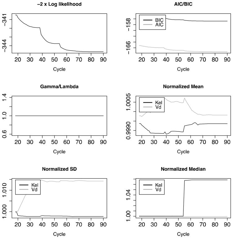
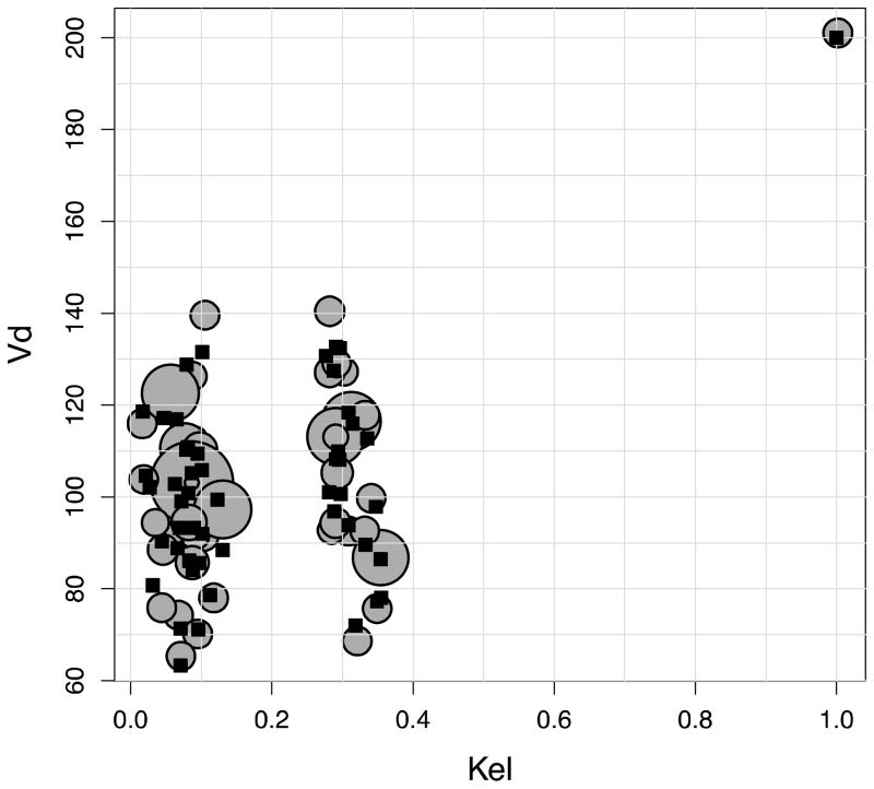
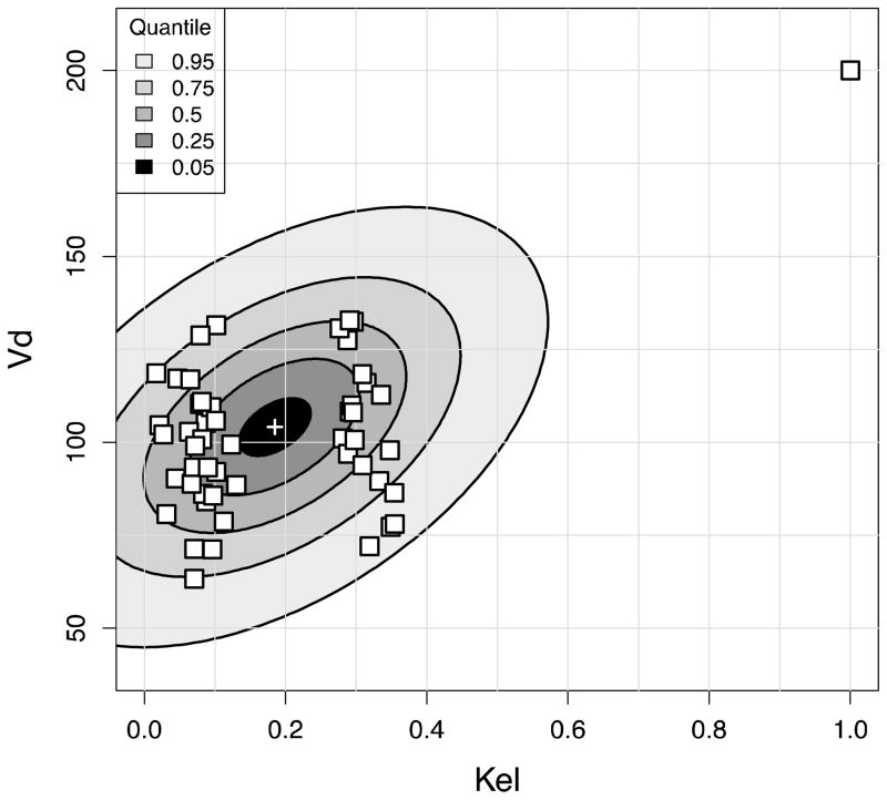
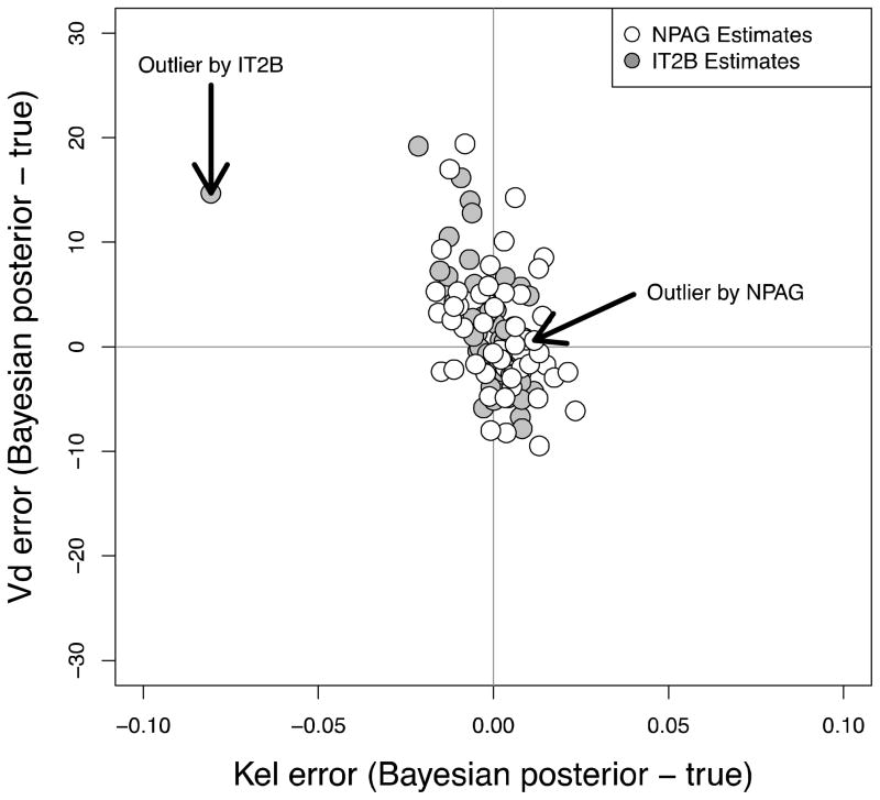
NPAG converged after 90 iterations, and IT2B converged after 4 iterations, both in less than a minute. A representative Pmetrics cycle plot for the NPAG run is shown in Figure 1. This plot was generated with the plot(cycle.1) command, after loading all the output from NPAG with NPload(1). Summary statistics for the final simulated data set with the outlier, and the NPAG and the IT2B final distributions are shown in Table 2. The summaries for NPAG and IT2B were obtained in Pmetrics by examining the final objects, also loaded with NPload and ITload. Both methods were able to discover accurately the true central tendencies and dispersions of the data. However, when it came to discovering the true bimodal distribution for Kel, and accurately describing the outlier, NPAG was far superior to IT2B, as expected from the properties of non-parametric analysis. As shown in Figure 2, the mean for the population distribution is found to be where no subject actually lies. Moreover, the assumed parametric (normal) population distribution from IT2B is unable to adequately fit the outlier. In Figure 3, the errors in the individual Bayesian posterior parameter estimates cluster around 0 for both IT2B and NPAG, except for the outlier, who is well described using the non-parametric approach, but very poorly described using the parametric approach. Both Figures 2 and 3 were generated with custom R code from Pmetrics objects (included in downloadable code at www.lapk.org/teaching.php), demonstrating that any analysis or plot is possible once the data are loaded into R.

Figure 1.

Standard Pmetrics cycle plot for NPAG to evaluate convergence. By default, the first 20% of the total cycle number are omitted from the plots to magnify the final cycles. All plots should approach a constant slope of 0 as convergence occurs. In this simulated example, there is no additional noise beyond assay noise, so gamma is one in all cycles.

Table 2.

Summaries of the simulated “true” final dataset with a single outlier, and the final cycle values from NPAG and IT2B

	True	NPAG	IT2B
Mean (SD)
Kel	0.19 (0.17)	0.19 (0.16)	0.18 (0.16)
Vd	102 (22.3)	104 (22.6)	104 (24.4)
Median
Kel	0.10	0.11	0.10
Vd	101	103	101
Kel-Vd correlation	0.50	0.48	0.48

Figure 2.

(A) Results of the NPAG fit. True parameter values from the simulated population are shown as black squares, with NPAG support points shown as circles whose size is an approximate multiple of the size of one square, proportionally increased according to the probability of each NPAG point. (B) Results of the IT2B fit. True parameter values are shown as white squares. Note the outlier in the upper right corner. The bivariate normal parameter distribution estimated by IT2B is depicted as ellipses of fading color corresponding to the percentile of the distribution. The white cross at the center is the mean.

Figure 3.

Bivariate errors in Bayesian posterior parameter estimates for each subject’s Kel and Vd when analyzed with NPAG (open circles) and IT2B (filled circles). The outlier subject is highlighted with arrows.

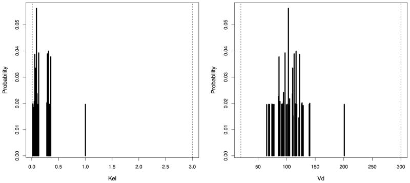
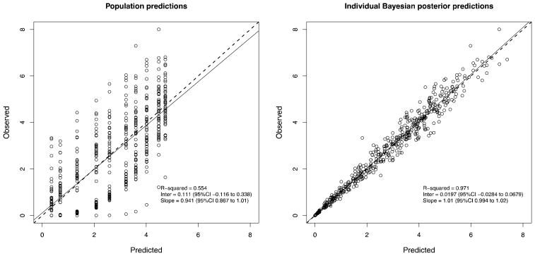
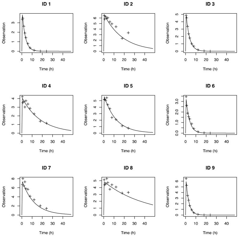
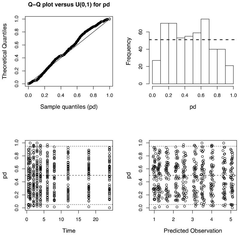
Figure 4 is a marginal plot of the final NPAG cycle population values for Kel and Vd, clearly demonstrating the two subpopulations for Kel and the outlier in both Kel and Vd. This plot was simply generated in Pmetrics with plot(final.1), again with final.1 automatically loaded using the NPload(1) command. The accuracy of predictions can be visualized in an observed vs. predicted plot, such as shown in Figure 5, or by plotting raw data for individual subjects vs. their full individual posterior predicted time-output profile, such as shown in Figure 6 for the first nine subjects. Numerous options are available for all these plotting functions, detailed within the R help file for each function. Finally, Figure 7 shows the normalized prediction discrepancies derived from simulating a further 1000 profiles from each of the 51 original subjects, and calculating the distribution of normalized prediction errors between each set of 1000 and its original, “seed” subject. This “internal” method of model validation was originally developed by Mentré et al,¹⁵ and has also been termed a standardized visual predictive check by Wang et al.¹⁴ It is also simple in Pmetrics to perform “external” model validation by using the model as a prior distribution to predict observations taken from new dataset, and this is detailed in the User’s Manual.¹²

Figure 4.

Standard Pmetrics marginal plot for Kel and Vd from final cycle population values estimated by NPAG. Dashed lines at the margins are the original ranges for each parameter specified for the run. The outlier is clearly visible at Kel=1.0 and Vd=200, as well as the bimodal distribution for Kel and unimodal distribution for Vd.

Figure 5.

Standard Pmetrics observed vs. predicted plots based on population predictions (left) or individual Bayesian posterior predictions.

Figure 6.

Standard Pmetrics plot for full individual Bayesian posterior time-output profiles from NPAG with superimposed observations (plus marks). For brevity, only the first 9 subjects are shown.

Figure 7.

Standard Pmetrics plot of prediction discrepancies (or standardized visual predictive check) for internal model validation using the simulator embedded within the PMdiag function and a multi-modal, multi-variate prior distribution of parameter values from the non-parametric population model, as described in the text. Expected distributions in the normal Q-Q plot (upper left) and histogram (upper right) are indicated by the reference lines. Distributions on the lower plots should ideally be evenly distributed between 0 and 1, with the 5^th, 50^th (median) and 95^th percentiles indicated by the reference lines. As expected from simulated data, the results in this figure show a very good model fit.

Discussion

Pmetrics is an R package for Unix and Windows that allows pharmacometric experts to use familiar input files to run parametric, and more uniquely, non-parametric population analyses of pharmacokinetic and pharmacodynamic data, including semi-parametric Monte Carlo simulation. In a simple example, we have highlighted the strengths that an accurate, reliable, and mature non-parametric approach can bring to the analysis of data: 1) easy discovery of unsuspected sub-populations (e.g. fast and slow metabolizers), and 2) accurate fitting of outliers, which does not obscure the true variability in a population that may not be sampled extensively enough for parametric methods to detect. We hope that members of the pharmacometric community will wish to add this powerful tool to their existing workflows.

A drawback to Pmetrics is that one must be familiar with R to use it. We have worked hard to minimize this requirement by including many standard plotting and data visualizing functions, but there is no doubt that more advanced R users will be able more readily to generate custom plots and analysis of the output from Pmetrics. There is usually tension between power and flexibility on the one hand, and ease of use on the other. We acknowledge that currently Pmetrics falls on the former side, but we are working to improve the balance, including the future option for users to interact with Pmetrics in a “point-and-click” fashion through a graphical user interface, which will facilitate learning and common tasks.

We have spent a lot of time documenting Pmetrics, both as a User’s Manual, and as help files within R. We have also made sample scripts, datasets, a template model library, video tutorials, and a discussion forum available on our website. It is our hope that Pmetrics will be a living project to which users may contribute useful and customized models and R code. For that reason all the R code is open-source and all components necessary to run Pmetrics are freely available.

Conclusion

Pmetrics is a Windows and Unix R package for non-parametric and parametric population modeling and simulation of pharmacokinetic and pharmacodynamic systems to improve therapeutic drug dosing in populations and individuals. We have shown here that its robust, reliable, and mature non-parametric approach to pharmacometrics, built on over three decades of work, is more adept than the parametric method at discovering unsuspected sub-groups and characterizing outlier subjects. Pmetrics brings a suite of standard, but customizable plotting functions to visualize output and diagnostics from the model fitting, and makes the data available for analysis using the full power and flexibility of R.

References

- 1.Barrett JS, Fossler MJ, Cadieu KD, Gastonguay MR. Pharmacometrics: a multidisciplinary field to facilitate critical thinking in drug development and translational research settings. J Clin Pharmacol. 2008;48(5):632–649. doi: 10.1177/0091270008315318. [DOI] [PubMed] [Google Scholar]
- 2.Neely M, Jelliffe R. Practical, individualized dosing: 21st century therapeutics and the clinical pharmacometrician. J Clin Pharmacol. 2010;50(7):842–847. doi: 10.1177/0091270009356572. [DOI] [PubMed] [Google Scholar]
- 3.Neely M, Jelliffe R. Practical therapeutic drug management in HIV-infected patients: use of population pharmacokinetic models supplemented by individualized Bayesian dose optimization. J Clin Pharmacol. 2008;48(9):1081–1091. doi: 10.1177/0091270008321789. [DOI] [PMC free article] [PubMed] [Google Scholar]
- 4.Schumitzky A. Nonparametric EM Algorithms for Estimating Prior Distributions. Applied Math and Computation. 1991;45:141–157. [Google Scholar]
- 5.Baek Y. An Interior Point Approach to Constrained Nonparametric Mixture Models. [Google Scholar]
- 6.Bustad A, Terziivanov D, Leary R, Port R, Schumitzky A, Jelliffe R. Parametric and nonparametric population methods: their comparative performance in analysing a clinical dataset and two Monte Carlo simulation studies. Clin Pharmacokinet. 2006;45(4):365–383. doi: 10.2165/00003088-200645040-00003. [DOI] [PubMed] [Google Scholar]
- 7.Kiefer J, Wolfowitz J. Consistency of the Maximum Likelihood Estimator in the Presence of Infinitely Many Incidental Parameters. The Annals of Mathematical Statistics. 1956;27(4):887–906. [Google Scholar]
- 8.Mallet A. A maximum likelihood estimation method for random coefficient regression models. Biometrika. 1986;73:645–656. [Google Scholar]
- 9.Jelliffe R, Bayard D, Milman M, Van Guilder M, Schumitzky A. Achieving target goals most precisely using nonparametric compartmental models and “multiple model” design of dosage regimens. Ther Drug Monit. 2000;22(3):346–353. doi: 10.1097/00007691-200006000-00018. [DOI] [PubMed] [Google Scholar]
- 10.Bayard DS. A forward method for optimal stochastic nonlinear and adaptive control. Auto Con IEEE Trans. 1991;36(9):1046–1053. [Google Scholar]
- 11.R Development Core Team. R project. R Foundation for Statistical Computing; 2011. [Accessed December 14, 2011]. R: A language and environment for statistical computing. Available at: http://www.R-project.org/ [Google Scholar]
- 12.Neely M. Pmetrics User’s Manual. [Accessed December 13, 2011];University of Southern California Laboratory of Applied Pharmacokinetics. Available at: http://www.lapk.org/pmetrics.php.
- 13.Goutelle S, Bourguignon L, Maire PH, Van Guilder M, Conte JE, Jelliffe RW. Population modeling and Monte Carlo simulation study of the pharmacokinetics and antituberculosis pharmacodynamics of rifampin in lungs. Antimicrob Agents Chemother. 2009;53(7):2974–2981. doi: 10.1128/AAC.01520-08. [DOI] [PMC free article] [PubMed] [Google Scholar]
- 14.Wang DD, Zhang S. Standardized Visual Predictive Check Versus Visual Predictive Check for Model Evaluation. J Clin Pharmacol. 2011 doi: 10.1177/0091270010390040. [DOI] [PubMed] [Google Scholar]
- 15.Mentré F, Escolano S. Prediction discrepancies for the evaluation of nonlinear mixed-effects models. J Pharmacokinet Pharmacodyn. 2006;33(3):345–367. doi: 10.1007/s10928-005-0016-4. [DOI] [PMC free article] [PubMed] [Google Scholar]
- 16.Wickham H. devtools: Tools to make developing R code easier. R package version 0.4. [Accessed 2011];The comprehensive R archive network (CRAN) 2011 Available at: http://CRAN.R-project.org/package=devtools.
- 17.D’Agostino R. Transformation to Normality of the Null Distribution of G 1. Biometrika. 1970;57(3):679–681. [Google Scholar]