Robust principal component analysis-based four-dimensional computed tomography

Abstract

The purpose of this paper for four-dimensional (4D) computed tomography (CT) is threefold. (1) A new spatiotemporal model is presented from the matrix perspective with the row dimension in space and the column dimension in time, namely the robust PCA (principal component analysis)-based 4D CT model. That is, instead of viewing the 4D object as a temporal collection of three-dimensional (3D) images and looking for local coherence in time or space independently, we perceive it as a mixture of low-rank matrix and sparse matrix to explore the maximum temporal coherence of the spatial structure among phases. Here the low-rank matrix corresponds to the ‘background’ or reference state, which is stationary over time or similar in structure; the sparse matrix stands for the ‘motion’ or time-varying component, e.g., heart motion in cardiac imaging, which is often either approximately sparse itself or can be sparsified in the proper basis. Besides 4D CT, this robust PCA-based 4D CT model should be applicable in other imaging problems for motion reduction or/and change detection with the least amount of data, such as multi-energy CT, cardiac MRI, and hyperspectral imaging. (2) A dynamic strategy for data acquisition, i.e. a temporally spiral scheme, is proposed that can potentially maintain similar reconstruction accuracy with far fewer projections of the data. The key point of this dynamic scheme is to reduce the total number of measurements, and hence the radiation dose, by acquiring complementary data in different phases while reducing redundant measurements of the common background structure. (3) An accurate, efficient, yet simple-to-implement algorithm based on the split Bregman method is developed for solving the model problem with sparse representation in tight frames.

1. Introduction

Respiratory motion can degrade the image quality of computed tomography (CT), and consequently cause substantial errors in the dose delivery for thoracic and upper abdominal tumors in radiation therapy (Xing et al 2006, Jiang et al 2008). With time-resolved data acquisition, four-dimensional (4D) CT possesses an unprecedented capability for accurate patient imaging and treatment planning in spite of organ/tumor motion (Vedam et al 2003, Low et al 2003, Keall et al 2004, Rietzel et al 2005, Li et al 2005).

Two methodologies for 4D CT algorithms exist. In the first one, different temporal phases (each phase corresponding to a 2D or 3D spatial image) are essentially considered as independent phases in image reconstruction. For example, with an external respiratory signal for synchronization, the acquired projection data are binned into different phases according to amplitude or phase-angle sorting (Lu et al 2006), after which the reconstruction is performed for each phase. There is no correlation between phases in reconstruction to this point. To alleviate the view-aliasing artifacts due to the reduced number of projections, the image registration based on a deformable model of respiratory motion can be used either in image space (Rueckert et al 1999) or in data space with an artifact-free reference image (Li et al 2007). The similar ideas also appear in other 4D imaging techniques (Schreibmann et al 2008), such as 4D positron emission tomography (PET) (Nehmeh et al 2003).

In contrast, in the second methodology, the ‘time’ dimension is explicitly incorporated into the reconstruction algorithm. That is, all the phases are treated as a single entity. An apparent reason for this temporal fusion is that the images at different phases are intrinsically interconnected to each other due to some underlying physical or biological mechanism. As a result, this spatiotemporal synthesis feature is highly desirable in any truly 4D algorithm. For example, a spatiotemporal regularization via non-local means is utilized to enforce the temporal similarity between two consecutive phases in 4D CT (Jia et al 2010). Another unified spatiotemporal strategy is also considered in 4D inverse planning for intensity-modulated radiation therapy (Lee et al 2009).

In this paper, we will present a different spatiotemporal model for 4D CT from matrix perspective, namely the robust PCA (principal component analysis)-based 4D CT model (RPCA-4DCT model). That is, instead of viewing the 4D object as a temporal collection of three-dimensional (3D) images and looking for local coherence in time or space independently, we perceive it as a mixture of low-rank matrix and sparse matrix to explore the maximum temporal coherence of spatial structure among phases. Here the low-rank matrix corresponds to the ‘background’ or reference state, which is stationary over time or similar in structure; the sparse matrix stands for the ‘motion’ or time-varying component, e.g., heart motion in cardiac imaging, which is often either approximately sparse itself or can be sparsified in the proper basis. Here the image sparsity is enforced in the wavelet tight frame domain rather than itself (Ron and Shen 1997).

In addition, we will also introduce a dynamic data acquisition scheme to maximize the utility of the RPCA-4DCT model and develop an efficient solution algorithm. Specifically, a temporally spiral scanning procedure can potentially maintain the similar reconstruction accuracy with far fewer projections of the data that are complementary at different phases to avoid redundant measurements of the common background structure; while being accurate, the split Bregman method offers an extremely efficient, yet simple-to-implement strategy for solving a class of general l₁-type problems, including the proposed RPCA-4DCT model (Goldstein and Osher 2009, Cai et al 2009).

The RPCA-4DCT model is motivated by the recent work for data analysis in statistics, i.e. RPCA (Candès et al 2009). That is, with the data matrix consisting of a low-rank part and a sparse part, both can be (almost) exactly recovered by minimizing the sum of the nuclear norm of the low-rank component and l₁ norm of the sparse component subject to certain assumptions (incoherence conditions). The similar models have been considered in several applications, such as video surveillance (Candès et al 2009), face recognition (Candès et al 2009), video denoising (Ji et al 2010), and others (Peng et al 2010, Liu et al 2010, Min et al 2010, Zhu et al 2010, Zhang et al 2010, Wu et al 2010). A key difference between the RPCA-4DCT model and RPCA and most existing applications is that the available data here are tomographic measurements linked to the object through some ill-posed system matrix rather than directly from the object itself. Although the required incoherence conditions for guaranteeing the success of RPCA to exactly recover both low-rank and sparse matrices cannot be rigorously justified in such an ill-posed inverse problem, we will show in this paper that the RPCA-4DCT model indeed offers not only improved overall image quality for 4D CT, but also quite satisfactory decomposition into the background and the motion/change. Moreover, the RPCA-4DCT model can be augmented when in conjunction with the tight frame transform, a dynamic data acquisition scheme pertinent to 4D CT, and the split Bregman method. Finally, we remark that the proposed RPCA-4DCT model is a general model that can be potentially applicable in other imaging problems aiming at motion reduction or/and change detection besides 4D CT, such as multi-energy CT, cardiac MRI, and hyperspectral imaging.

2. Models and algorithms

2.1. Model

The 4D object to be imaged can be viewed as a temporal sequence of 2D or 3D spatial images, i.e.

$$X=\{x_j,j\le n_t\},$$ (2.1)

where X is the 4D object with a temporal index j and x_j corresponds to one of n_t phases, that is usually a piecewise-constantly discretized image in space. Note that the respiratory cycle is generally assumed in order to acquire enough data for reconstructing each phase in the cycle (Vedam et al 2003). However, this temporal periodicity is not necessary in the model formulation; thus, it is not assumed in (2.1). The assumption we impose on the model in this study is fairly natural and practical, i.e. the temporal variation of X in space is ‘sparse’ (under certain sparsifying transform) with respect to a ‘stationary’ background. Shortly, this assumption will be quantified as a matrix decomposition model, i.e. the RPCA-4DCT model, with each component characterized in the proper norm.

The available data at each phase are

$$Y=\{y_j≔A_j{x}_j+N_j,j\le n_t\}.$$ (2.2)

Here y_j is assumed to be the x-ray transform of x_j with certain measurement noise N_j, and A_j corresponds to the system matrix that can be assembled according to line integrals in the image space between source–detector pairs (Buzug 2008). Originally, the system matrix should be independent of the index j since it is usually determined solely by the scanning geometry. In the following we will introduce a dynamic scanning strategy with the consequent dependence on j to explore the possibility of 4D low-dose CT with fewer projections of data. On the other hand, the model and the algorithm discussed later also apply to other formulations of the system matrix, such as the Fourier-based one (Buzug 2008).

2.1.1. Existing models

In 4D CT, one tries to reconstruct the 4D object X from its projection data Y. An apparent way is to reconstruct x_j solely from y_j for each phase, and then post-process x_j altogether for artifact reduction (if necessary), i.e.

$$\{\begin{array}{cc}{x}_j=\underset{x_j}{\text{arg min}}{\Vert A_j{x}_j-y_j\Vert }^2+R(x_j),\hfill & j\le n_t\hfill \\ X=F(x_1,\dots ,x_j,\dots ,x_{n_t}).\hfill & \hfill \end{array}$$ (2.3)

The first equation of (2.3) represents the solution of x_j through the minimization of a least-squares data fidelity term and a regularization term R on the image x_j. Here the regularization is necessary for reducing the image artifact that may be due to the noise or the insufficient number of projections. This is a well-known iterative reconstruction strategy that is commonly used in algebraic reconstruction techniques (ART) when the system matrix is underdetermined, i.e. the number of data is less than the number of unknowns (Buzug 2008). For comparison of models, L₂ regularization and total variation (TV) regularization (Rudin et al 1992) will be employed, i.e. the following with i the spatial index:

$${\Vert x_j\Vert }^2={\displaystyle \sum _i}{x}_{\mathit{\text{ij}}}^2\text{ and }|\nabla x_j|={\displaystyle \sum _i}\sqrt{{({\partial }_x{x}_{\mathit{\text{ij}}})}^2+{({\partial }_y{x}_{\mathit{\text{ij}}})}^2+{({\partial }_z{x}_{\mathit{\text{ij}}})}^2}.$$ (2.4)

In the second equation of (2.3), F represents the post-processing, for example, to alleviate the view-aliasing artifacts or smooth the image variation between phases. A commonly used method is based on the deformable model (Rueckert et al 1999). Alternatively, when an artifact-free reference image is available, the image deformable model can also be used to ‘smooth’ the data first, and then followed by the phase-wise reconstruction (Li et al 2007).

An immediate benefit of the model (2.3) is that the problem is computationally minimal in the sense that it is almost equivalent to solve a few CT problems with some extra cost for pre-/post-processing. However, this model is fundamentally defective. That is, the interplay between spatial images among different phases is considered a pure image registration problem rather than a truly 4D reconstruction. As a result, the embedded features that are available only through a 4D model can never be revealed otherwise, e.g., through (2.3).

Therefore, one should incorporate spatial images at different phases as a single entity into the reconstruction model. The next question is what should the model look like?

A natural thought is to consider the following:

$$X=\underset{X}{\text{arg min}}{\displaystyle \sum _j}[{\Vert A_j{x}_j-y_j\Vert }^2+R(x_j)]+R_t(X),$$ (2.5)

where the reconstruction of x_j at different phases is performed simultaneously with an additional regularization term in time, i.e. R_t(X). That is, the data fidelity term is enforced at all phases, while the solution is regularized both spatially and temporally. Note that despite the simultaneous consideration of all phases, the regularization is however independently carried out locally in space and time. In section 3, we will adopt TV regularization in both space and time for comparison of models (Weickert and Schnörr 2001). That is, with the alternative representation of X in pixels rather than phases, e.g., x_i consisting of all phases at the ith pixel,

$$X=\{x_i,i\le n_s\},$$ (2.6)

the temporal TV regularization is defined as

$$|{\nabla }_t{x}_i|={\displaystyle \sum _j|{\partial }_t{x}_{\mathit{\text{ij}}}|.}$$ (2.7)

Then, the model (2.5) becomes the following with TV regularization in both space and time:

$$X=\underset{X}{\text{arg min}}{\displaystyle \sum _j}{\Vert A_j{x}_j-y_j\Vert }^2+{\lambda }_1{\displaystyle \sum _j}|\nabla x_j|+{\lambda }_2{\displaystyle \sum _i}|{\nabla }_t{x}_i|.$$ (2.8)

Although (2.8) is a way to model 4D CT as a 4D reconstruction problem, this model is still not very satisfactory in the sense that the spatiotemporal regularization is enforced ‘locally’, while in reality the 4D entity is a ‘global’ mixture in time and space.

2.1.2. Robust PCA-based 4D CT model

The major contribution of this work is to introduce a new spatiotemporal 4D model from the matrix perspective, i.e. the RPCA-4DCT model in short. That is, X parameterized conventionally in space via (2.1) or in time via (2.6) can be represented in a matrix with row dimension for the spatial variable and column dimension for the temporal variable:

$$X=[x_1\cdots x_j\cdots x_{n_t}].$$ (2.9)

As mentioned earlier, the respiratory motion can be regarded as a sequence of spatial images with different temporal sparse ‘motion’ or ‘change’ from a common ‘background’. Motivated by this observation, we consider the following natural low-rank and sparse decomposition of X:

$$X=X_1+X_2.$$ (2.10)

In (2.10), X₁ is the low-rank matrix component for modeling the stationary background of X. Note that X₁ is assumed to resemble each other rather than to be constant in time, which can be naturally characterized as a low-rank matrix mathematically. On the other hand, X₂ is the sparse matrix component for modeling the sparse deviation from the background X₁. Here the sparsity can be the image itself or the image under the proper sparsifying transform that will be discussed shortly.

Accordingly, when the temporal change of images is sparse in the original representation, we consider the following matrix minimization problem for the RPCA-4DCT model:

$$(X_1,X_2)=\underset{(X_1,X_2)}{\text{arg min}}{\Vert A(X_1+X_2)-Y\Vert }^2+{\lambda }_{*}{\Vert X_1\Vert }_{*}+{\lambda }_1{\Vert X_2\Vert }_1,$$ (2.11)

where A represents a linear operator composed of system matrices {A_j}, the nuclear norm for penalizing the rank of the matrix X₁ (altogether for all phases) is defined as the sum of its singular values {σ_k} with the regularizing parameter λ_*, and the l₁ norm for promoting the sparsity of X₂ (independently for each phase) is simply the absolute sum of its entries with the regularizing parameter λ₁, i.e.

$${\Vert X_1\Vert }_{*}={\displaystyle \sum _k}{\sigma }_k\text{ and }{\Vert X_2\Vert }_1={\displaystyle \sum _j}\left({\displaystyle \sum _j}|X_{2,\mathit{\text{ij}}}|\right).$$ (2.12)

Compared with (2.8), the RPCA-4DCT model via (2.11) offers a unified treatment in time and space, while each 4D component is characterized via the proper norm, such as (2.12). The gain of the overall reconstruction quality via the RPCA-4DCT model will be apparent in section 3. In addition, the separation of X₂ from the background X₁ is a unique feature of the RPCA-4DCT model with captured dynamic details that would sometimes be crucial but hardly recognizable visually.

On the other hand, there may be concern that the computational cost would increase dramatically due to the simultaneous reconstruction of X at all phases. In section 2.3, we will address this question with an efficient algorithm, which shows that the collective optimization via (2.8) or (2.11) costs roughly the same as independent optimizations via (2.3).

2.1.3. Connection with prior works

The RPCA-4DCT model is motivated by RPCA for data analysis in statistics (Candès et al 2009). In Candès et al (2009), a model to recover principal component X₁ (modeled by a low-rank matrix) from data X with outliers X₂ (modeled by a sparse matrix) is converted to the following minimization problem when certain incoherence conditions are satisfied:

$$\begin{array}{c}(X_1,X_2)=\underset{(X_1,X_2)}{\text{arg min}}{\Vert X_1\Vert }_{*}+r{\Vert X_2\Vert }_1\hfill \\ \text{Subject to }{X}_1+X_2=Y,\hfill \end{array}$$ (2.13)

where r is shown to be the following for the matrix with n₁ rows and n₂ columns, so that no tuning parameter is necessary:

$$r=\frac{1}{\sqrt{\text{max}(n_1,n_2)}}.$$ (2.14)

2.1.4. RPCA-4DCT model revisited

Physical images usually have sparse structure under some carefully constructed dictionary, if not in the original representation. In this study, we find that the tight frame system derived from Ron and Shen (1997) and Daubechies et al (2003) in general serves the purpose in terms of low-rank and sparse decomposition. As a result, the RPCA-4DCT model via (2.11) is revised as

$$(X_1,X_2)=\underset{(X_1,X_2)}{\text{arg min}}{\Vert A(X_1+X_2)-Y\Vert }^2+{\lambda }_{*}{\Vert X_1\Vert }_{*}+{\lambda }_1{\Vert {\mathit{\text{WX}}}_2\Vert }_1,$$ (2.15)

where W represents the framelet analysis operator with W_TW = I. In this study, a multilevel tight framelet decomposition without downsampling under the Neumann (symmetric) boundary condition is used with piecewise linear framelets (Chai and Shen 2007, Cai et al 2008).

A key difference between our RPCA-4DCT model (2.15) and RPCA (2.13) and most existing applications is that the available data set Y here is the tomographic data of X generated by some system matrix rather than directly from X itself. As a result, the required incoherence conditions for guaranteeing the success of RPCA cannot be rigorously justified in such an ill-posed inverse problem. Another difference is that the sparsity of X₂ is enforced in the transform domain in the RPCA-4DCT model, while it is in the original image domain in RPCA. Besides, the component X₂ here is for modeling the motion or the change which is often crucial for CT, and the data/image noise is controlled by the data fidelity term; in contrast, in some applications of RPCA, the component X₂ is considered to be the noise that is of less interest.

The sparsity of images under tight framelets has been successfully used to solve many image restoration tasks including image denoising, image deblurring, image inpainting, etc (e.g. Cai et al 2008, 2009, Chai and Shen 2007). Most importantly, tight framelets are redundant systems, which lead to robust image representations. Therefore, partial loss and noise of the data in CT can be tolerated without adverse effects. Moreover, the filters in piecewise linear B-spline framelets are the first and second discrete difference operators, respectively, and the multiscale structure of the framelets enables their multilevel correspondences. These difference operators are well organized in such a way that they have the unitary property W_TW = I. Altogether, the piecewise linear B-spline framelet can provide more difference operators than traditional partial differential equation-based methods such as TV regularization, and hence it can handle images with abundant structures.

Another benefit using tight framelet systems is the availability of more efficient numerical methods to solve the resulting minimization (2.15). We will use the split Bregman method to solve (2.15), and there is a system of linear equations to be solved in each iteration of the split Bregman method. Since A is usually underdetermined and W_TW = I, it can be verified that the coefficient matrix of the resulting linear system has clustering eigenvalues. Therefore, the system of linear equations can be solved efficiently by the conjugate gradient (CG) method, and CG gives the exact solution after only a few steps.

On the other hand, with a priori knowledge of the noise in (2.2), the RPCA-4DCT model (2.15) can be further augmented by characterizing the first term (the data fidelity term) with the appropriate norm. For example, if the data come with impulse noise, l₁ norm is particularly suitable for characterizing such outliers (Alliney 1992, Nikolova 2002, Chan and Esedoglu 2005, Gao and Zhao 2010). In this study, for simplicity, we assume Gaussian data noise and penalize the data fidelity term with L₂ norm.

Finally, we remark that when the considered 4D object changes drastically in time, it can be reformulated into a few overlapping 4D objects according to the properly chosen temporal windows. Consequently, the overall reconstruction is with respect to the weighted sum of 4D components (Ji et al 2010).

2.2. Dynamic scanning

One of the major practical concerns of CT is its ionizing radiation dose. For instance, it has been estimated that although CT studies constitute only 4%of all radiological procedures, they account for 40% of the radiation dose delivered (Shrimpton and Edyvean 1998); furthermore, ‘CT could account for as much as 60% of manmade radiation exposures to Americans’ (Linton et al 2003). Tremendous effort has been devoted to dose reduction (Xing et al 2006, Jiang et al 2008, Pan et al 2009, Fahimian et al 2010, Wang et al 2010). For example, as a theoretically justified methodology, ‘interior tomography’, an internal region of interest (ROI) can be exactly reconstructed only from local projection data directly associated with this ROI, which would conventionally require the whole body x-ray illumination (Wang et al 2010, Ye et al 2007, Kudo et al 2008).

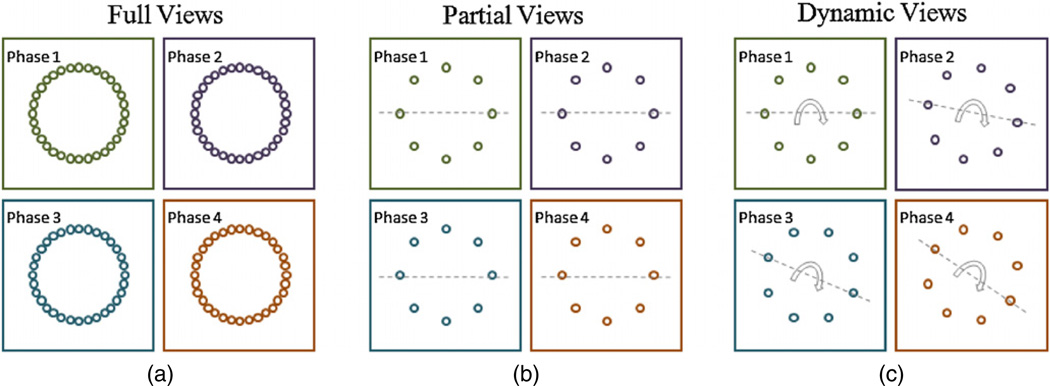
Here we propose a dynamic scanning procedure pertinent to 4D CT that can potentially offer further dose reduction through the reduced number of projections. This dynamic scanning is temporally ‘spiral’ as illustrated in figure 1.

Figure 1.

An illustration example on scanning procedures for 4D CT. (a) ‘Full views’ corresponds to full data acquisition with 32 projections for each phase; (b) ‘partial views’ corresponds to partial data acquisition with 8 projections, which is temporally stationary in each phase; (c) ‘dynamic views’, again with 8 projections, is, however, dynamically variant among phases, so that any view can be swept in some phase within a full dynamic cycle while avoiding redundant measurements of the common background structure at different phases. In this example one data acquisition cycle is synchronized with 4D images with four phases. Note that no temporal periodicity of the images is assumed.

While figure 1(a) shows full views of data (‘full views’), figure 1(b) shows a temporally stationary data acquisition scheme with the reduced number of views that is stationary over time (‘partial views’). In contrast, figure 1(c) shows a dynamic scanning procedure (‘dynamic views’). In ‘dynamic views’, the positioning of acquired views differs between consecutive phases, however changes periodically so that each view is covered at least once during a dynamic period of scanning. In this way, the redundant measurements of the common background structure at different phases can be avoided. Note that we do not assume the temporal periodicity of images.

The potential advantage of the proposed ‘dynamic views’ (figure 1(c)) is that it can achieve comparable image quality with a fewer number of views than ‘full views’ (figure 1(a)), or provide better image quality with the same number of views as ‘partial views’ (figure 1(b)). A heuristic explanation is that the acquired views in one period can be fused into a dataset of full views so that the tangible data for each phase are from full views rather than partial views. What are missing in the data acquired from ‘dynamic views’ compared with ‘full views’ mostly corresponds to the redundant measurements of the stationary background.

Moreover, ‘dynamic views’ is practically feasible as long as the object to be imaged can be regarded as a single temporal phase within the time period of each data acquisition. Next we will use the reported parameters in Vedam et al (2003) to illustrate its applicability in 4D CT for respiratory motion. That is, assuming that (1) the 4D object of interest is one respiratory cycle with 6 s in time, (2) the scanner rotation time for full views is 1.5 s, (3) a fraction of the entire views are to be used for each phase, i.e. one eighth, then it is safe to consider the 4D model with up to 32 phases.

In contrast, in the standard scanning procedure, the over-sampled views of data are first acquired without pre-arrangement of the scanning according to phases, and then are binned into different phases according to amplitude or phase-angle sorting using an external respiratory signal (Lu et al 2006). Note that the 4D objects to be imaged have to assume certain temporal periodicity in order to carry out the synchronized binning. Compared with this standard scanning procedure, the proposed dynamic scanning scheme has the following apparent advantages: (1) no external respiratory signal is necessary, (2) the 4D objects do not have to be periodic, (3) most importantly, the carefully designed periodic data acquisition scheme provides the almost equivalent image quality as the full-view acquisition. On the other hand, it is synergetic with other potential scanning procedures for dose reduction, such as multi-source interior tomography (Wang et al 2009).

2.3. Algorithm

In this section, we consider the solution of the RPCA-4DCT model via the following optimization:

$$(X_1,X_2)=\underset{(X_1,X_2)}{\text{arg min}}\frac{1}{2}{\Vert A(X_1+X_2)-Y\Vert }^2+{\lambda }_{*}({\Vert X_1\Vert }_{*}+r{\Vert {\mathit{\text{WX}}}_2\Vert }_1),$$ (2.16)

where r is defined by (2.14), and λ_* is the only regularizing parameter to be determined.

Here we adopt an accurate, efficient, but simple-to-implement algorithm for solving the non-differentiable l₁-type problems, such as (2.16), namely the split Bregman method, that is essentially equivalent to the augmented Lagrangian method; however, it was independently developed from a different perspective to improve the ROF model (Goldstein and Osher 2009, Osher et al 2005). In particular, the tight frame regularized split Bregman method is implemented here (Cai et al 2009). That is, equation (2.16) can be exactly solved through the following simple iterative scheme with X₁⁰ = X₂⁰ = 0, f⁰ = 0, d₁⁰ = υ₁⁰ = 0 and d₂⁰ = υ₂⁰ = 0:

$$\{\begin{array}{c}(X_1^{k+1},X_2^{k+1})=\underset{(X_1,X_2)}{\text{arg min}}{\Vert A(X_1+X_2)-Y+f^k\Vert }^2+{\mu }_{*}{\Vert X_1-d_1^k+{\upsilon }_1^k\Vert }^2+{\mu }_1{\Vert {\mathit{\text{WX}}}_2-d_2^k+{\upsilon }_2^k\Vert }^2,\hfill \\ d_1^{k+1}=\underset{d_1}{\text{arg min}}\frac{1}{2}{\Vert X_1^{k+1}+{\upsilon }_1^k-d_1\Vert }^2+\frac{{\lambda }_{*}}{{\mu }_{*}}{\Vert d_1\Vert }_{*},\hfill \\ d_2^{k+1}=\underset{d_2}{\text{arg min}}\frac{1}{2}{\Vert {\mathit{\text{WX}}}_2^{k+1}+{\upsilon }_2^k-d_2\Vert }^2+\frac{r{\lambda }_{*}}{{\mu }_1}{\Vert d_2\Vert }_1,\hfill \\ {\upsilon }_1^{k+1}={\upsilon }_1^k+X_1^{k+1}-d_1^{k+1},\hfill \\ {\upsilon }_2^{k+1}={\upsilon }_2^k+{\mathit{\text{WX}}}_2^{k+1}-d_2^{k+1},\hfill \\ f^{k+1}=f^k+A(X_1^{k+1}+X_2^{k+1})-Y.\hfill \end{array}$$ (2.17)

The convergence of this iterative scheme when the variables are vectors has been established in Cai et al (2009). Although the split Bregman method here by (2.17) is for matrix variables, the convergence can be obtained by mimicking the proofs in Cai et al (2009).

The first step of (2.17) corresponds to one iteration step in a typical differentiable L₂ minimization, and the solution is simply from its optimal condition. In implementation, A and W are regarded as linear operators rather than matrices. For efficiency, CG is utilized in which only the evaluations of linear operators on X_j are necessary, such as A_j X₁^j and WX²_j, without the explicit formulation and inversion of the whole system. As we have mentioned before, it can be verified that the considered matrix system has clustering eigenvalues. Therefore, CG gives the exact solution after only a few iterations. Note that if only a single iteration is used in CG, (2.17) can be viewed as a typical example of operator splitting methods (Combettes and Wajs 2005, Hale et al 2008, Zhang et al 2009). However, it is found here that the conventional CG with a few iterations is more realistic in terms of reconstruction accuracy and convergence speed, which was also mentioned in Jia et al (2010).

The second step of (2.17) can be exactly solved by the so-called singular value thresholding (SVT) algorithm (Cai et al 2010). That is,

$$d_1^{k+1}=D_{{\lambda }_{*}/{\mu }_{*}}(X_1^{k+1}+{\upsilon }_1^k),$$ (2.18)

where the thresholding is with respect to singular values σ of the input matrix, i.e.

$$D_{\tau }(X)≔U·\text{diag}(\text{max}(\sigma -\tau ,0))·V^T,\text{ with }X=U·\text{diag}(\sigma )·V^T.$$ (2.19)

For this step, the major computational cost is from singular value decomposition (SVD), which can be expensive in the overall scheme (2.17). However, it is sufficient to consider this step by SVD in this study since the number of columns of the matrix considered here (corresponding to the number of phases in 4D object) is so small that SVT (2.19) via SVD is computationally negligible overall. In the case of a large number of phases, the fast SVT without SVD can be used (Cai and Osher 2010).

The solution to the third step of (2.17) is given by the so-called shrinkage formula, i.e.

$$d_2^{k+1}=T_{r{\lambda }_{*}/{\mu }_1}({\mathit{\text{WX}}}_2^{k+1}+{\upsilon }_2^k),$$ (2.20)

with

$$T_{\tau }(X)≔\text{sgn}(X)·\text{max}(|X|-\tau ,0).$$ (2.21)

Note that the shrinkage formula (2.21) is a scalar operation for each entry of X, while SVT (2.19) is a global operation on X.

Regarding the parameters in (2.17), the following are recommended:

$$r=\frac{1}{\sqrt{\text{max}(n_1,n_2)}}\text{ and }{\mu }_{*}={\mu }_1={\lambda }_{*},$$ (2.22)

where n₁ (n₂) are the number of rows (columns) of the matrix X. Here the choice of r is supported by the rigorous analysis for RPCA (Candès et al 2009) although the theory assumptions cannot be justified rigorously here due to the system matrix A. Furthermore, it is found that λ_* ∈[0.1, 10] generally provides the satisfactory performance in terms of both accuracy and speed.

In the proposed algorithm via (2.17), the dominant component is to solve L₂ problems in the first step. Due to its iterative nature, empirically it is not necessary to solve each CG step with very high accuracy in order for the whole loop to achieve fast convergence besides the fact that the system has a good condition number as mentioned before. We found that CG with 10 to 20 inner iterations is adequate for (2.17) to have the acceptable reconstruction accuracy within 50 outer iterations.

The similar split Bregman strategy as (2.17) can be used for solving other models in section 2.1. Another advantage of the split Bregman method is that the computation cost for the RPCA-4DCT model (2.15) is similar to the corresponding L₁-type 4D models, such as (2.8) with TV regularization in both time and space, or a temporally independent sequence of 3D models, such as (2.3) with TV regularization in space.

3. Results

The purpose here is twofold: (1) to compare different models and (2) to justify the proposed dynamic scanning.

To simplify the discussion, let ‘L₂’ (‘TV’) be the 3D model that solves 4D CT by each individual phase, i.e. (2.3) with L₂ (TV) regularization; let ‘TV+TVt’ be the 4D model that solves 4D CT as a single entity, i.e. (2.8) with TV regularization in both space and time; let the RPCA-4DCT model be the proposed matrix model that solves 4D CT as a single entity, i.e. (2.15) with a low-rank component and a sparse component (in tight frames). Note that we do not compare here with the standard filtered backprojection (without regularizing solutions), which generally gives worse accuracy than ‘L₂’ when reconstructing with insufficient number of views.

In this proof-of-concept study, for simplicity, the spatial dimension is 2D rather than 3D, i.e. a 128 by 128 spatial grid. Here 32 temporal phases are adopted for the justified reasons in section 2.2. With the parallel scanning geometry, the length of the detectors with 256 detector pixels is equal to the side length of the spatial square domain, and ‘full views’ consist of 256 projections. The reconstructions with three different data acquisition schemes (figure 1) will be compared: ‘full views’ corresponds to the use of all data; ‘partial views’ corresponds to the use of 32 projections that is temporally stationary in phases; ‘dynamic views’ corresponds to the use of 32 projections that is dynamically adjusted among phases so that any view is covered in some phase within a full dynamic period while avoiding redundant measurements of the common background. Here one data acquisition cycle is synchronized with eight phases and the data are acquired with four cycles.

Except ‘L₂’, which is differentiable and therefore can be solved with iterations involving only one step that is similar to the first step of (2.17), all aforementioned other models can be solved through split Bregman iterations similar to (2.17). As a result, since the major computational cost in all models is on the L₂ step similar to the first step in (2.17), the total computation time approximately only depends on the number of iterations. It is found that roughly 20–50 iterations together with the parameters specified by (2.22) are sufficient. In particular, all models except ‘L₂’ are similar in computational cost, while ‘L₂’ fails to achieve the satisfactory accuracy (comparing with other models) regardless of the number of iterations.

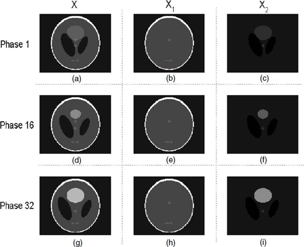
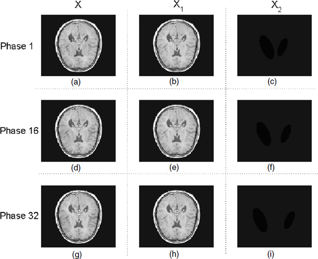
Two spatiotemporal phantoms are used for evaluation. Phantom 1 is utilized for evaluating the reconstruction with motion, while the purpose of phantom 2 is for change detection.

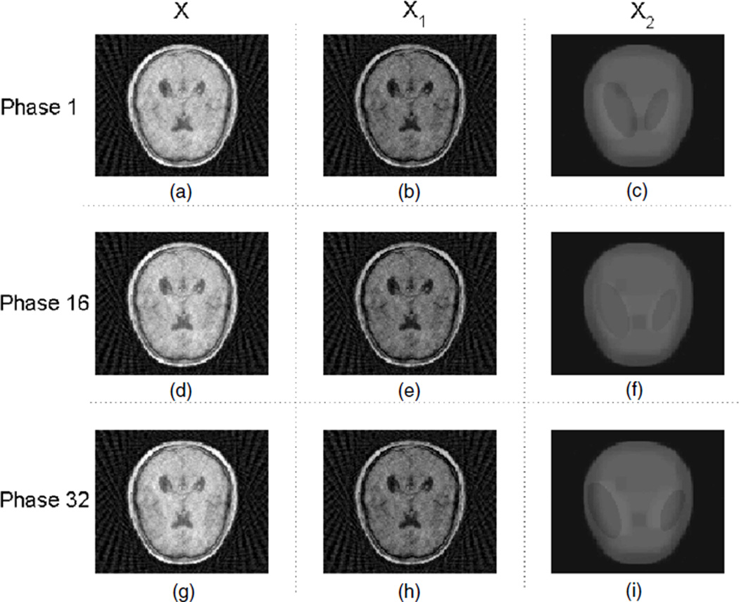
Phantom 1 is to mimic a half respiratory cycle with the cardiac motion, which is based on the modified Shepp–Logan phantom that consists of piecewise constant regions (figure 2). The cardiac phases are generated according to the model proposed in Wang et al (2002). The temporal variations consist of (1) the cardiac model: the intensity increase and the area change of the top circle (with a relatively large diameter); (2) the small deformation: the vertical movement of the lower central circle (with a relatively small diameter), and (3) the lung motion: the horizontal movement of two ellipses (with a relatively low contrast) apart from each other.

Figure 2.

Phantom 1 for 4D CT; (a), (b) and (c) are the image X, the background of the image X₁ and the motion/change of the image X₂, respectively, at phase 1, i.e. X = X₁ + X₂. Similarly, (d), (e) and (f) correspond to X, X₁ and X₂ at phase 16, and (g), (h) and (i) correspond to X, X₁ and X₂ at phase 32.

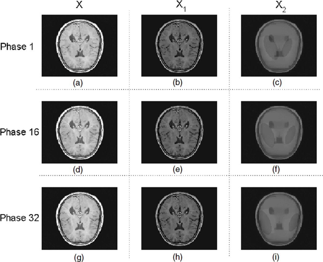
Phantom 2 is to model the case with small temporal variations, which can be even hardly recognizable by human eyes (figure 3). It is based on a MRI brain image and the temporal variations consist of the horizontal movement of two ellipses (with a relatively very low contrast) apart from each other.

Figure 3.

Phantom 2 for 4D CT; (a), (b) and (c) are the image X, the background of the image X₁ and the motion/change of the image X₂, respectively, at phase 1, i.e. X = X₁ + X₂. Similarly, (d), (e) and (f) correspond to X, X₁ and X₂ at phase 16, and (g), (h) and (i) correspond to X, X₁ and X₂ at phase 32.

3.1. Model comparison

In this section, a small fraction of full views are used, i.e. one eighth of the full data (32 projections). Specifically, we adopt ‘dynamic views’ as the data acquisition scheme (figure 1(c)).

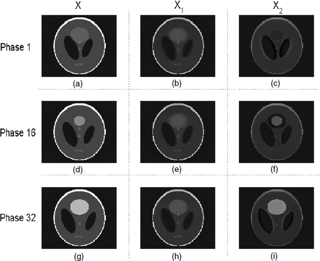
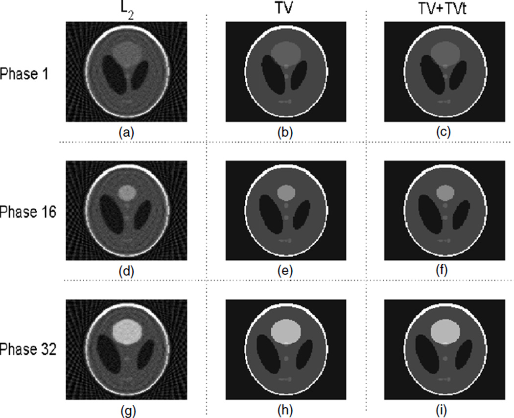
For phantom 1, the result from the RPCA-4DCT model is shown in figure 4, which clearly shows that the RPCA-4DCT model is not only able to recover images but also provide automatic image decomposition into the background (that is mathematically low-rank) and the variation (that is sparse under tight frame transform). In contrast, the results from other models are shown in figure 5. Since phantom 1 is in favor of TV regularization due to its components in piecewise constants, ‘TV’ and ‘TV+TVt’ offer the equivalent image quality although the RPCA-4DCT model is slightly better in terms of reconstruction errors (table 1).

Figure 4.

Reconstructed images with the RPCA-4DCT model for phantom 1; (a), (b) and (c) are the total image X, the low-rank component X₁ and the sparse component (in tight frames) X₂, respectively, at phase 1, i.e. X = X₁ + X₂. Similarly, (d), (e) and (f) correspond to X, X₁ and X₂ at phase 16, and (g), (h) and (i) correspond to X, X₁ and X₂ at phase 32.

Figure 5.

Reconstructed images with other various models for phantom 1; (a), (b) and (c) are from ‘L₂’, ‘TV’ and ‘TV+TVt’, respectively, at phase 1. Similarly, (d), (e) and (f) correspond to the above models at phase 16, and (g), (h) and (i) correspond to the above models at phase 32.

Table 1.

Reconstruction accuracy from various models (with ’dynamic views’). The quantities are the quotient differences between the ground truth X⁰ and the reconstructed images X, i.e. ‖X − X⁰‖/‖X⁰‖ with ‖·‖ L₂ norm.

Phantom	L2	TV	TV+TVt	LR+TF
1	0.314	0.008	0.006	0.004
2	0.197	0.076	0.040	0.022

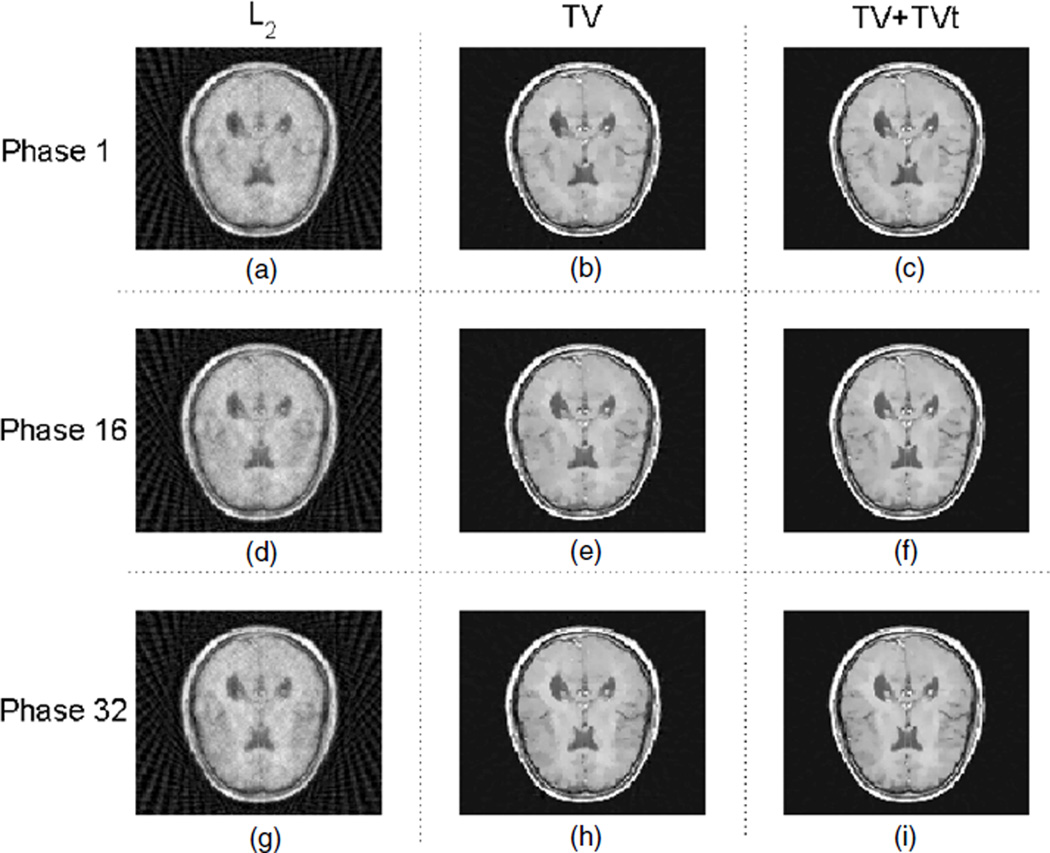
On the other hand, the result from the RPCA-4DCT model for phantom 2 is shown in figure 6, which again indicates that the matrix model is not only superior in the overall image quality, but also able to capture these small features that would be impossible otherwise. For comparison, the results from other models are shown in figure 7. With temporal TV regularization, ‘TV+TVt’ provides better overall image quality than ‘TV’ both visually (figure 7) and quantitatively (table 1), which however is worse than the RPCA-4DCT model. The blurred or smoothed details are apparent for either ‘TV’ or ‘TV+TVt’. Besides, neither clearly shows the temporal variations, which in contrast are available through the RPCA-4DCT model without extra computational cost.

Figure 6.

Reconstructed images with the RPCA-4DCT model for phantom 2; (a), (b) and (c) are the total image X, the low-rank component X₁ and the sparse component (in tight frames) X₂, respectively, at phase 1, i.e. X = X₁ + X₂. Similarly, (d), (e) and (f) correspond to X, X₁ and X₂ at phase 16, and (g), (h) and (i) correspond to X, X₁ and X₂ at phase 32.

Figure 7.

Reconstructed images with other various models for phantom 2; (a), (b) and (c) correspond to ‘L₂’, ‘TV’ and ‘TV+TVt’, respectively, at phase 1. Similarly, (d), (e) and (f) correspond to the above models at phase 16, and (g), (h) and (i) correspond to the above models at phase 32.

Note that although the decomposition via the RPCA-4DCT model is non-unique, the variations are clearly captured as in figures 4 and 6. Furthermore, such a clear decomposition with captured details via the RPCA-4DCT model is usually not available through the post-processing of images from other models, such as the simple subtraction of images with respect to the first phase.

3.2. Scanning comparison

The reconstructions are performed on phantom 2 with the RPCA-4DCT model to compare three different data acquisition schemes (figure 1), i.e. ‘full views’ with 256 projections for each phase, ‘partial views’ with 32 projections for each phase that are temporally invariant in terms of positioning of projections, and ‘dynamic views’ with 32 projections for each phase that are dynamically variant so that each view is available for some phase in a full scanning cycle. Here one data acquisition cycle is synchronized with eight phases and the data are acquired with four cycles.

The reconstruction results for ‘dynamic views’, ‘partial views’ and ‘full views’ are presented in figures 6, 8 and 9, respectively, and the quantitative reconstruction accuracy is summarized in table 2. The results clearly show that ‘dynamic views’ has a great potential for dose reduction since it offers a satisfactory accuracy with only a small fraction of the full data.

Figure 8.

Reconstructed images with the RPCA-4DCT model for phantom 2 with ‘partial views’.

Figure 9.

Reconstructed images with the RPCA-4DCT model for phantom 2 with ‘full views’.

Table 2.

Reconstruction accuracy from various data scanning schemes with the RPCA-4DCT model. The quantities are the quotient differences between the ground truth X⁰ and the reconstructed images X, i.e. ‖X − X⁰‖/‖X⁰‖ with ‖·‖ L₂ norm.

Phantom	Partial views	Dynamic views	Full views
2	0.187	0.022	0.005

References

- Alliney S. Digital filters as absolute norm regularizers. IEEE Trans. Signal Process. 1992;40:1548–1562. [Google Scholar]
- Buzug T. Computed Tomography: From Photon Statistics to Modern Cone-Beam CT. Berlin: Springer; 2008. [Google Scholar]
- Cai JF, Candès EJ, Shen Z. A singular value thresholding algorithm for matrix completion. SIAM J. Optim. 2010;20:1956–1982. [Google Scholar]
- Cai JF, Chan RH, Shen Z. A framelet-based image inpainting algorithm. Appl. Comput. Harmon. Anal. 2008;24:131–149. [Google Scholar]
- Cai JF, Osher S. Fast singular value thresholding without singular value decomposition. UCLA CAM Report 10–24. 2010 [Google Scholar]
- Cai JF, Osher S, Shen Z. Split Bregman methods and frame based image restoration. Multiscale Model. Simul. 2009;8:337–369. [Google Scholar]
- Candès EJ, Li X, Ma Y, Wright J. Technical Report. Stanford University; 2009. Robust principal component analysis? [Google Scholar]
- Chai A, Shen Z. Deconvolution: a wavelet frame approach. Numer. Math. 2007;106:529–587. [Google Scholar]
- Chan TF, Esedoglu S. Aspects of total variation regularized L1 function approximation. SIAM J. Appl. Math. 2005;65:1817–1837. [Google Scholar]
- Combettes PL, Wajs VR. Signal recovery by proximal forward-backward splitting. Multiscale Model. Simul. 2005;4:1168–1200. [Google Scholar]
- Daubechies I, Han B, Ron A, Shen Z. Framelets: MRA-based constructions of wavelet frames. Appl. Comput. Harmon. Anal. 2003;14:1–46. [Google Scholar]
- Fahimian BP, Mao Y, Cloetens P, Miao J. Low dose x-ray phase-contrast and absorption CT using equally-sloped tomography. Phys. Med. Biol. 2010;55:5383–5400. doi: 10.1088/0031-9155/55/18/008. [DOI] [PubMed] [Google Scholar]
- Gao H, Zhao HK. Multilevel bioluminescence tomography based on radiative transfer equation: part 2. Total variation and l1 data fidelity. Opt. Express. 2010;18:2894–2912. doi: 10.1364/OE.18.002894. [DOI] [PubMed] [Google Scholar]
- Goldstein T, Osher S. The split Bregman algorithm for l1 regularized problems. SIAM J. Imaging Sci. 2009;2:323–343. [Google Scholar]
- Hale E, Yin W, Zhang Y. Fixed-point continuation for l1-minimization: methodology and convergence. SIAM J. Optim. 2008;19:1107–1130. [Google Scholar]
- Ji H, Liu C, Shen Z, Xu Y. Robust video denoising using low rank matrix completion. IEEE Conf. Computer Vision and Pattern Recognition (CVPR); San Francisco. 2010. [Google Scholar]
- Jia X, Lou Y, Dong B, Tian Z, Jiang S. 4D computed tomography reconstruction from few-projection data via temporal non-local regularization. Lect. Not. Comput. Sci. 2010;(6361):143–150. doi: 10.1007/978-3-642-15705-9_18. [DOI] [PubMed] [Google Scholar]
- Jiang SB, Wolfgang J, Mageras GS. Quality assurance challenges for motion-adaptive radiation therapy: gating, breath holding, and four dimensional computed tomography. Int. J. Radiat. Oncol. Biol. Phys. 2008;71:S103–S107. doi: 10.1016/j.ijrobp.2007.07.2386. [DOI] [PubMed] [Google Scholar]
- Keall PJ, Starkschall G, Shukla H, Forster KM, Ortiz V, Stevens CW, Vedam SS, George R, Guerrero T, Mohan R. Acquiring 4D thoracic CT scans using a multislice helical method. Phys. Med. Biol. 2004;49:2053–2067. doi: 10.1088/0031-9155/49/10/015. [DOI] [PubMed] [Google Scholar]
- Kudo H, Courdurier M, Noo F, Defrise M. Tiny a priori knowledge solves the interior problem in computed tomography. Phys. Med. Biol. 2008;53:2207–2231. doi: 10.1088/0031-9155/53/9/001. [DOI] [PubMed] [Google Scholar]
- Lee L, Ma Y, Ye Y, Xing L. Conceptual formulation on four-dimensional inverse planning for intensity modulated radiation therapy. Phys. Med. Biol. 2009;54:N255–N266. doi: 10.1088/0031-9155/54/13/N01. [DOI] [PMC free article] [PubMed] [Google Scholar]
- Li T, Koong A, Xing L. Enhanced 4D cone-beam CT with inter-phase motion model. Med. Phys. 2007;34:3688–3695. doi: 10.1118/1.2767144. [DOI] [PubMed] [Google Scholar]
- Li T, Schreibmann E, Thorndyke B, Tillman G, Boyer A, Koong A, Goodman K, Xing L. Radiation dose reduction in four-dimensional computed tomography. Med. Phys. 2005;32:3650–3660. doi: 10.1118/1.2122567. [DOI] [PubMed] [Google Scholar]
- Linton OW, Fred A, Mettler FA. National conference on dose reduction in CT, with an emphasis on pediatric patients. Am. J. Roentgenol. 2003;181:321–329. doi: 10.2214/ajr.181.2.1810321. [DOI] [PubMed] [Google Scholar]
- Liu G, Lin Z, Yu Y. Robust subspace segmentation by low-rank representation. Proc. 26th Int. Conf. on Machine Learning (ICML); Haifa, Israel. 2010. [Google Scholar]
- Low D, et al. A method for the reconstruction of four-dimensional synchronized CT scans acquired during free breathing. Med. Phys. 2003;30:1254–1263. doi: 10.1118/1.1576230. [DOI] [PubMed] [Google Scholar]
- Lu W, Parikh PJ, Hubenschmidt JP, Bradley JD, Low DA. A comparison between amplitude sorting and phase-angle sorting using external respiratory measurement for 4D CT. Med. Phys. 2006;33:2964–2974. doi: 10.1118/1.2219772. [DOI] [PubMed] [Google Scholar]
- Min K, Zhang Z, Wright J, Ma Y. Decomposing background topics from keywords by principal component pursuit. Proc. ACM Int. Conf. on Information and Knowledge Management (CIKM); Toronto, Canada. 2010. [Google Scholar]
- Nehmeh SA, Erdi YE, Rosenzweig KE, Schoder H, Larson SM, Squire OD, Humm JL. Reduction of respiratory motion artifacts in PET imaging of lung cancer by respiratory correlated dynamic PET: methodology and comparison with respiratory gated PET. J. Nucl. Med. 2003;44:1644–1648. [PubMed] [Google Scholar]
- Nikolova M. Minimizers of cost-functions involving nonsmooth data fidelity terms. Application to the processing of outliers. SIAM J. Numer. Anal. 2002;40:965–994. [Google Scholar]
- Osher S, Burger M, Goldfarb D, Xu J, Yin W. An iterative regularization method for total variation-based image restoration. Multiscale Model. Simul. 2005;4:460–489. [Google Scholar]
- Pan X, Sidky EY, Vannier M. Why do commercial CT scanners still employ traditional, filtered back-projection for image reconstruction? Inverse Problems. 2009;25 doi: 10.1088/0266-5611/25/12/123009. 123009. [DOI] [PMC free article] [PubMed] [Google Scholar]
- Peng Y, Ganesh A, Wright J, Xu W, Ma Y. RASL: robust alignment by sparse and low-rank decomposition for linearly correlated images. IEEE Conf. Computer Vision and Pattern Recognition (CVPR); San Francisco. 2010. [DOI] [PubMed] [Google Scholar]
- Rietzel E, Pan T, Chen GT. Four-dimensional computed tomography: image formation and clinical protocol. Med. Phys. 2005;32:874–889. doi: 10.1118/1.1869852. [DOI] [PubMed] [Google Scholar]
- Rueckert D, Sonoda LI, Hayes C, Hill DLG, Leach MO, Hawkes DJ. Non-rigid registration using free-form deformations: application to breast MR images. IEEE Trans. Med. Imaging. 1999;18:712–721. doi: 10.1109/42.796284. [DOI] [PubMed] [Google Scholar]
- Ron A, Shen Z. Affine systems in L2(Rd): the analysis of the analysis operator. J. Funct. Anal. 1997;148:408–447. [Google Scholar]
- Rudin L, Osher S, Fatemi E. Nonlinear total variation based noise removal algorithms. J. Phys. D: Appl. Phys. 1992;60:259–268. [Google Scholar]
- Schreibmann E, Thorndyke B, Li T, Wang J, Xing L. Four-dimensional image registration for image-guided radiotherapy. Int. J. Radiat. Oncol. Biol. Phys. 2008;71:578–586. doi: 10.1016/j.ijrobp.2008.01.042. [DOI] [PMC free article] [PubMed] [Google Scholar]
- Shrimpton PC, Edyvean S. CT scanner dosimetry. Br. J. Radiol. 1998;71:1–3. doi: 10.1259/bjr.71.841.9534691. [DOI] [PubMed] [Google Scholar]
- Vedam SS, Keall PJ, Kini VR, Mostafavi H, Shukla HP, Mohan R. Acquiring a four-dimensional computed tomography dataset using an external respiratory signal. Phys. Med. Biol. 2003;48:45–62. doi: 10.1088/0031-9155/48/1/304. [DOI] [PubMed] [Google Scholar]
- Wang G, Ye Y, Yu H. Interior tomography and instant tomography reconstruction from truncated limited angle projection data. 7697658 B2. US Patent. 2010 doi: 10.1155/2008/427989. [DOI] [PMC free article] [PubMed]
- Wang G, Yu HY, Ye YB. A scheme for multisource interior tomography. Med. Phys. 2009;36:3575–3781. doi: 10.1118/1.3157103. [DOI] [PMC free article] [PubMed] [Google Scholar]
- Wang G, Zhao S, Heuscher D. A knowledge based cone beam x-ray CT algorithm for dynamic volumetric cardiac imaging. Med. Phys. 2002;29:1807–1822. doi: 10.1118/1.1494989. [DOI] [PubMed] [Google Scholar]
- Weickert J, Schnörr C. Variational optic flow computation with a spatio-temporal smoothness constraint. J. Math. Imaging Vis. 2001;14:245–255. [Google Scholar]
- Wu L, Ganesh A, Shi B, Matsushita Y, Wang Y, Ma Y. Robust photometric stereo via low-rank matrix completion and recovery. Proc. Asian Conf. on Computer Vision; Queenstown, New Zealand. 2010. [Google Scholar]
- Xing L, Thorndyke B, Schreibmann E, Yang Y, Li TF, Kim GY, Luxton G, Koong A. Overview of image-guided radiation therapy. Med. Dosim. 2006;31:91–112. doi: 10.1016/j.meddos.2005.12.004. [DOI] [PubMed] [Google Scholar]
- Ye YB, Yu HY, Wei YC, Wang G. A general local reconstruction approach based on a truncated Hilbert transform. Int. J. Biomed. Imaging. 2007;(2007):63634. doi: 10.1155/2007/63634. [DOI] [PMC free article] [PubMed] [Google Scholar]
- Zhang X, Burger M, Bresson X, Osher S. Bregmanized nonlocal regularization for deconvolution and sparse reconstruction. UCLA CAM Report 09-03. 2009 [Google Scholar]
- Zhang Z, Liang X, Ganesh A, Ma Y. TILT: transform invariant low-rank textures. Proc. Asian Conf. on Computer Vision; Queenstown, New Zealand. 2010. [Google Scholar]
- Zhu G, Yan S, Ma Y. Proc. ACM Multimedia. Firenze: Italy; 2010. Image tag refinement towards low-rank, content-tag prior and error sparsity. [Google Scholar]