Abstract
The correct segmentation of blood vessels in optical coherence tomography (OCT) images may be an important requirement for the analysis of intra-retinal layer thickness in human retinal diseases. We developed a shape model based procedure for the automatic segmentation of retinal blood vessels in spectral domain (SD)-OCT scans acquired with the Spectralis OCT system. The segmentation procedure is based on a statistical shape model that has been created through manual segmentation of vessels in a training phase. The actual segmentation procedure is performed after the approximate vessel position has been defined by a shadowgraph that assigns the lateral vessel positions. The active shape model method is subsequently used to segment blood vessel contours in axial direction. The automated segmentation results were validated against the manual segmentation of the same vessels by three expert readers. Manual and automated segmentations of 168 blood vessels from 34 B-scans were analyzed with respect to the deviations in the mean Euclidean distance and surface area. The mean Euclidean distance between the automatically and manually segmented contours (on average 4.0 pixels respectively 20 µm against all three experts) was within the range of the manually marked contours among the three readers (approximately 3.8 pixels respectively 18 µm for all experts). The area deviations between the automated and manual segmentation also lie within the range of the area deviations among the 3 clinical experts. Intra reader variability for the experts was between 0.9 and 0.94. We conclude that the automated segmentation approach is able to segment blood vessels with comparable accuracy as expert readers and will provide a useful tool in vessel analysis of whole C-scans, and in particular in multicenter trials.
OCIS codes: (170.4500) Optical coherence tomography; (110.6880) Three-dimensional image acquisition; (100.0100) Image processing; (100.3008) Image recognition, algorithms and filters
1. Introduction
Optical coherence tomography (OCT) has revolutionized the in vivo imaging capacities in ophthalmology. The technique uses low coherence infrared light to visualize the reflectance of retinal structures in depth, similar to ultrasound. Since the early days about 20 years ago, technical advances in image quality and acquisition have made this technique crucial in the diagnostic procedure of many retinal and optic nerve disorders. The transition from Time-Domain (TD-OCT) to Spectral-Domain (SD-OCT) based OCT systems increased sensitivity, resolution (from 15 µm axial resolution to 6 µm) and recording speed (from 400 axial scans/s to 40000 axial scans/s) [1]. In contrast to the image quality of modern devices, image analysis tools are still quite restricted. Most commercial OCT devices currently perform only the segmentation of the entire retina or segmentation of the retinal nerve fiber layer (RNFL). It is of note though that the high resolution of SD-OCT scans theoretically allows for the analysis of more structures, including all discernible intra-retinal layers, blood vessels, druses, and fluid filled regions. However, a meaningful analysis requires the identification and segmentation of all of these structures in the same OCT B-scan.
The analysis of retinal blood vessels can be important not only in the diagnosis of various retinal diseases like diabetic retinopathy or glaucoma, it may also be an important tool to align different images taken from patients at different clinical visits. In addition, the RNFL thickness measurement can be made more accurate if the vessels are separated from the actual nerve fibers by a reliable segmentation method. However, manual segmentation of small retinal structures like blood vessels is extremely time consuming, and reliability is limited due to inter- and intra-grader variability. Due to the huge amount of data to be analyzed in a C-scan, it is practically impossible to perform segmentation tasks by an expert in clinical routine.
To make the amount of data available for routine diagnostics, automated segmentation algorithms may be the solution, as they can reduce analysis time and increase reliability for repeatable and quantitative results.
Most published vessel segmentation approaches are based on fundus images. For example, a thresholding based method was proposed by Hoover et al. [2], where the fundus image is examined in pieces and the pieces are tested for a number of criteria, and the algorithm is driven by a matched filter response. Budai et al. [3] proposed a multiscale algorithm for automatic segmentation, which uses a Gaussian resolution hierarchy and an efficient neighborhood analysis approach on each level to segment vessels of different diameters. A neural network classification based method was described by Sinthanayothin et al. [4], where the inputs for a multilayer perceptron neuronal network were derived from a principal component analysis (PCA) of the fundus image and edge detection of the first component of PCA. However, all these examples of vessel segmentation approaches were only performed on fundus images.
The first segmentation method based on OCT images was presented by Niemeijer et al. [5]. The method is based on a supervised pixel classification of a 2-D projection created by information from certain automatically segmented retinal layers in a 3-D volume. The performance of the method depends on the robustness of the retinal layer segmentation and axial segmentation is not performed. A second classification based method to segment blood vessels in lateral direction was proposed by Xu et al. [6], in which a training set of vessel and non-vessel A-scans is created to segment vessel A-scans in unseen images (i.e. all images that were not used for training) by classification. Again, an axial segmentation of the blood vessels is not performed.
The first method to segment vessels in lateral and axial direction was proposed by Lee et al. [7]. The algorithm is based on a 3-D graph search. A graph is composed of a set of nodes and a set of arcs and is created from the image, where the nodes correspond to the image pixels and the arcs connect the nodes. The retinal blood vessel segmentation in the 3-D graph search method was based on a vessel model. To create the triangular mesh of an initial 3-D vessel model in x- and y-direction, the OCT projection image was calculated by averaging two retinal layer surfaces. Additional information for the model creation concerning the depth position in z-direction was gathered from optical Doppler tomography images.
In this paper we present for the first time the use of a shape model approach for automated segmentation of retinal blood vessels with cross sectional B-scans, where a-priori knowledge about the shape characteristics of retinal blood vessels is used. The shape model is used to segment objects in unseen images, where plausible variations of the model are created and compared to the image data until the object fits best. The proposed method performs segmentation in lateral and axial direction compared to most other approaches where only the lateral position is determined.
2. Materials and methods
OCT images were acquired from 8 different healthy eyes for statistical shape model creation and from 13 different healthy eyes for algorithm evaluation using the Spectralis OCT system (Heidelberg Engineering, Heidelberg, Germany) with an axial resolution of 4 µm, a transversal resolution of 14 µm and an acquisition speed of 40000 A-Scans/sec. The volume and circular scan protocols were used for acquisition of images with sizes of 768 × 496, 1024 × 496 pixels and 1536 × 496 pixels. The image data were exported as raw data, and no processing steps were done by the OCT device itself. The algorithms were written in C/C++.
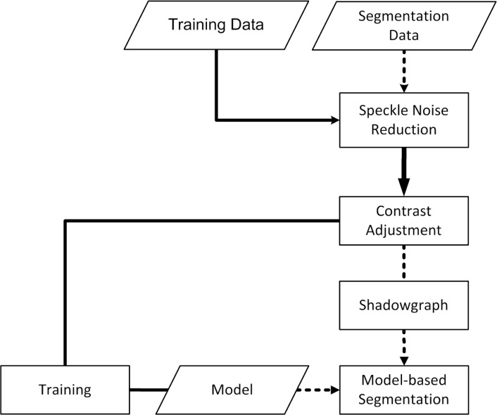
The development of the algorithm consisted of two major parts. In the first part, a statistical shape model (SSM) was created in a training step via the point distribution model, in which training data were segmented manually by so called landmarks. In the second part, the actual segmentation procedure was performed on unseen images by creating a shadowgraph of the scan to assign the lateral vessel position followed by the active shape model (ASM) method to segment the vessels in vertical direction. Pre-processing procedures, such as noise reduction and contrast adjustment were done prior to the segmentation. The basic segmentation algorithm flow is summarized in Fig. 1 .
Fig. 1.
The segmentation algorithm consists of two parts. First, a statistical shape model is trained via the point distribution model in the solid procedure flow. The actual segmentation process of unseen images is then performed with the creation of a shadow graph and with the active shape model method based on the data of the statistical shape model from the first step (dotted arrows in the flow chart).
2.1. Speckle noise reduction
Different speckle noise reduction approaches have been developed in the past years and were used by OCT segmentation algorithms for suppression. Fernández [8] showed that denoising by a nonlinear complex diffusion filter [9] is an essential processing step for detection of fluid-filled region boundaries by a deformable contour model (also known as snakes). Kajić et al. [10] applied a dual-tree wavelet algorithm [11] for image data denoising for intra-retinal layer segmentation.
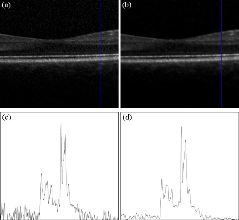
Our algorithm uses a general Bayesian estimation based method for speckle noise reduction, in which the image is projected into the logarithmic space to estimate the noise-free data using a conditional posterior approach [12]. Figure 2 shows that the method provides effective speckle noise reduction on Spectralis OCT scans in our set up. The algorithm was processed on a section of 300 A-Scans centered on the human healthy macula and provides effective noise reduction while preserving thin retinal layers and small retinal blood vessels.
Fig. 2.
(a) Input B-scan recorded with the Spectralis OCT centered on a healthy human macula. (b) Processed speckle noise suppression with the Bayesian estimation approach. (c) Sampled A-scan of the raw image. The noise component is strong and blurs the original signal. (d) Sampled A-scan of the suppressed image. The noise component is much lower and the retinal structures are preserved.
2.2. Statistical shape model creation
The starting point of creating a statistical shape model is the generation of manually segmented samples. In our project, the retinal blood vessel shape model is based on the work of Cootes et al., who proposed a point distribution model (PDM), in which the shape of a manually segmented object is defined by points, so called landmarks [13]. An object is defined by a vector of image coordinates of n landmarks , in which the number of landmarks must be the same for all objects of the sample. Corresponding landmarks of the manual segmentations are aligned by performing translation, rotation and scaling using a Procrustes analysis.
The mean shape vector represents the mean object shape of the sample with s elements, where the landmarks of all objects are averaged by Eq. (1):
| (1) |
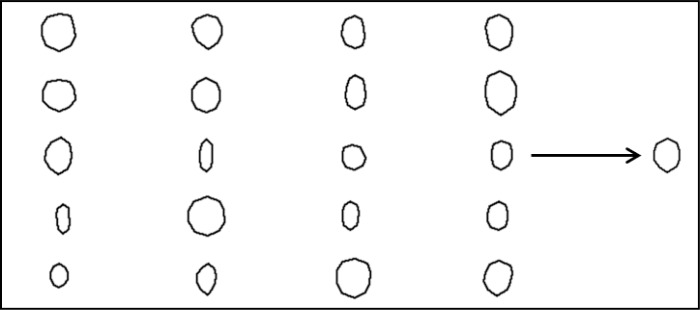
The entire set of manually segmented shapes consists of 52 blood vessels from 8 B-scans from 8 different healthy eyes. Figure 3 shows 20 blood vessel shapes of the entire set of 52 blood vessels, in which each shape is defined by 10 landmarks in equal distance along the boundary. The resulting mean shape of the set of shapes is shown on the right side of Fig. 3.
Fig. 3.
On the left side, 20 shapes of different manually segmented blood vessels are shown. On the right side, the mean blood vessel shape is shown that has been obtained by averaging the 10 landmarks for all shapes of the set.
To reduce the number of dimensions of the training set, a principal component analysis (PCA) is applied to find a small set of modes that describes the shape variation. The deviation of each shape dxt from the mean shape is calculated by Eq. (2) and the covariance matrix is calculated by Eq. (3):
| (2) |
| (3) |
An eigendecomposition gives the principal modes of variation pl (eigenvectors) and the corresponding variances λl (eigenvalues) of S. The matrix P is built from each eigenvector ordered in descending order of the eigenvalues λl in Eq. (4):
| (4) |
The goal of calculating a PCA is to reduce the number of parameters in the SSM. The t modes of variation are chosen until the accumulated variance λl reaches a certain ratio. Here the common ratio of 0.98 was chosen, and the retinal blood vessel model includes 98% of the training set shape variations.
A shape instance x of the training set is then approximated by Eq. (5):
| (5) |
New conformable shapes of the model are created by varying the shape coefficients in b within suitable limits in order to position the population of landmarks between three times the standard deviation in Eq. (6):
| (6) |
By defining pose parameters, an instance of the model is created in the image frame by Eq. (7):
| (7) |
where is a scaling by s and a rotation by θ, and defines the center position.
2.3. Grey-level appearance model creation
Regions surrounding corresponding landmarks are similar in different images. Therefore, we used a formulation for the analysis of the grey-level appearance [14]. On each landmark i of each image Ij the grey-level profile gij of np pixel length is sampled on the normal to the boundary (see Fig. 4 ). We used a profile length of 25 pixels. The kth grey-level element of the profile is sampled by Eq. (8):
Fig. 4.
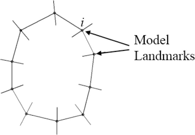
The grey-level variations are sampled on the normal of each landmark for all blood vessel shapes of the training set. The grey-level appearance is used to search for blood vessel objects in unseen images.
| (8) |
The grey-level profile will be normalized in order to be less sensitive to variations in a profile by Eq. (9):
| (9) |
For each landmark i the mean profile and the covariance matrix are calculated in Eq. (10) and Eq. (11):
| (10) |
| (11) |
2.4. Search for objects in unseen images
In unseen images, blood vessel contours are calculated by the active shape model (ASM) [14], in which the statistical shape model and the grey-level variations of each landmark are combined. The segmentation process starts by placing the mean shape nearby the object to be segmented. The shape coefficients are changed iteratively until the object fits optimally. We have included grey-level profile models for each landmark ensuring that the ASM searches for regions that fit best to the profile models in new images. On each model landmark a profile is sampled with a larger length then the model profile (>np). The model profile is compared to the sampled profile to find the best position. We used the Mahalanobis distance to calculate the optimal fit position between the grey-level profile of the object in the new image and the model profile for each landmark i by Eq. (12):
| (12) |
where h(d) is a sub-interval of the model profile length np of the sampled profile (length > np) centered at d [14]. Therefore, for each shape model landmark a vector with position movements results in Eq. (13):
| (13) |
The landmarks of the current model X should be moved to the best new locations (X + dX), which need to be within conformable possible object shape variations. This is achieved by finding the deviations in translation (dXc, dYc), rotation dθ and scale ds that fit best the current instance to the new positions (X + dX). This is done by the Procrustes analysis. The residual adjustments dx in the local model coordinate frame is given by Eq. (14):
| (14) |
This results in
| (15) |
where. To adjust the model points as closely to dx as possible, the changes of the shape coefficients db is defined by Eq. (16):
| (16) |
The segmentation process stops when changes to the current shape model instance are calculated. The ASM procedure is shown in Fig. 5 for one iteration.
Fig. 5.
Segmentation procedure with the active shape model for one iteration. The mean shape model is placed near the image object (left) and the grey-level profiles of the image are compared to the model profiles for each landmark (middle). The model parameters are updated to move the model to the best positions marked as crosses (right).
2.5. Initialization
An important prerequisite of the ASM segmentation procedure is that the initial model instance must be placed nearby the object in the unseen images. Otherwise, the algorithm will not be able to calculate the grey-level profiles of the vessels (see Fig. 5) to provide reliable results.
The easiest way to initialize the shape model would be by user interaction [15,16]. The mean shape is placed nearby the object manually. Such a manual initialization was proposed by Hug et al. [17] where the user defines a principal control polygon for the shape with a small number of landmarks. However, this procedure is time consuming and results in different segmentations, and is therefore not used in our algorithm.
To perform the initialization of the ASM automatically, we use a search strategy [18–20], in which parts are based on the initialization by a global genetic search algorithm [21,22]. The respective calculation steps are summarized below.
In relation to the blood vessel sizes the search space of an OCT image is large. The maximum resolution of a B-scan at the Spectralis OCT device is 1536 × 496 = 761856 pixels, but samples of the grey-level profiles on the normals of each landmark are just 25 pixels long.
The search strategy for retinal blood vessels is based on the initialization algorithm of [20]. The ASM optimization algorithm with the grey-level appearance model is used to find the initial pose and model parameters. The search algorithm starts with an initial population of shape model configurations. The best matching candidates survive and are reused in further estimation rounds. Candidates with the best configuration are used for initialization. The algorithm flow including pseudo-code is described in detail in [20].
As an important parameter, any available a-priori knowledge is used to narrow the range of possible configurations. In our case, the retinal structure intensity above and below vessels in an OCT A-scan differs compared to regions without vessels.
Wehbe et al. [23] determined the lateral blood vessel positions by a so called shadowgraph, where two basic processing steps are calculated. First, a retinal layer segmentation approach was performed to remove the upper retinal layers. Second, the sum of each A-scan was calculated, in which non-vessel A-scans got a large sum, whereas A-scans with vessel got a small sum. Hence, the lateral positions of the blood vessels were determined by the first derivative of a shadowgraph. However, the graph in our algorithm is not created by the sum but by the grey-level centers of each A-scan position x Eq. (17):
| (17) |
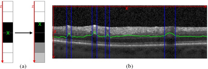
where h is the height of the B-scan image. Figure 6a shows the switch from a non-vessel A-scan to an A-scan with blood vessel and the effect on the grey-level center, and Fig. 6b shows the center positions for all A-scans of the image marked as green line. In A-scans with blood vessels, the peaks of the grey-level center are strong, which means that the lateral position and the width of the blood vessel shadows were determined by thresholding.
Fig. 6.
(a) The basic concept of the blood vessel shadowgraph with the grey-level centers of each A-scan. If the grey-level intensities are distributed in the same manner for the top and bottom region of the A-scan, the center lies in the middle. If the intensities got weaker due to the blood vessel shadows, the center migrates upward. (b) The grey-level centers processed for an entire B-scan are visualized as green line and the lateral segmentation of the blood vessel shadow is marked by blue vertical lines after thresholding.
The information of the shadowgraph was used to pre-estimate a number of initial search configurations and specific search ranges. The number of vessels, their locations in lateral direction, the widths and the locations in axial direction were approximated.
3. Results
The above described algorithm for automated blood vessel segmentation in B-scans taken with a Spectralis OCT device was evaluated for accuracy and reliability against three expert readers. In total, 168 retinal blood vessels in 34 OCT B-scans from 13 healthy eyes were manually segmented with markers. The first method to validate the performance of the algorithm was to compare the mean Euclidean distance between the contours defined by the algorithm and the contours defined by the experts. The method has been widely used to analyze algorithms for contour segmentation [9]. In a second validation step, we compared the areas of the blood vessels.
3.1. Mean Euclidian distance comparison
The mean Euclidean distance between a set of landmark points A (in this case A is the set of automated landmarks) and a second set M (in this case M is the set of expert’s landmarks) is calculated by Eq. (18):
| (18) |
where n is the number of landmarks within the set M and b within the set A. A(a) and M(m) represent the coordinate vector of the ath and mth landmark.
However, the mean Euclidean distance of Eq. (18) is not symmetric, . To get a symmetric definition, Eq. (19) is calculated:
| (19) |
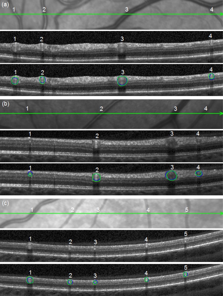
Figure 7 shows three B-scans together with the detail of the respective infrared fundus image. The segmentation results of the algorithm and one expert (expert 1) are shown as an example in order to visualize the obtained vessel contours. The average automated processing time for the three B-scans with 13 retinal blood vessels is about 9 seconds (Windows 7 Professional 64 bit, used one processor core of Intel Core i7 @ 2.8 GHz and 4 GB RAM). In contrast, expert readers need at least 120 seconds for all three B-scans.
Fig. 7.
Segmentation results of the automated approach (blue lines) and the clinical expert 1 (green lines). (a), (b) and (c) references to the B-scans.
The average distances of the measured contours within the group of experts and between each expert and the algorithm for all 168 blood vessels are detailed in Table 1 . The distances between algorithm and the three experts are on average approximately 4 pixels respectively (resp.) 20 µm. The minimal distance is 4.01 ± 1.97 pixel resp. 19.58 ± 9.76 µm between the automated method and expert 2. The maximal distance is 4.13 ± 1.967 pixel resp. 20.44 ± 10.06 µm between the automated method and expert 1. Compared to the distances among the expert readers, there is a small disagreement with a minimal inter-reader distance of 3.66 ± 1.73 pixel resp. 18.06 ± 8.91 µm and a maximal inter-reader distance of 3.85 ± 1.92 pixel resp. 19.67 ± 9.63 µm.
Table 1. Mean Euclidian distance between the measured vessel contours for the entire set of 168 blood vessels.
|
Mean Euclidean distance ± SD | ||
|---|---|---|
| Auto.—Expert 1 | Auto.—Expert 2 | Auto.—Expert 3 |
| 4.13 ± 1.97 pixel 20.44 ± 10.06 µm | 4.01 ± 1.97 pixel 19.58 ± 9.76 µm | 4.05 ± 1.74 pixel 20.05 ± 8.95 µm |
| Expert 1—Expert 2 | Expert 1—Expert 3 | Expert 2—Expert 3 |
|---|---|---|
| 3.85 ± 1.92 pixel 19.67 ± 9.63 µm | 3.66 ± 1.73 pixel 18.06 ± 8.91 µm | 3.72 ± 1.7 pixel 18.26 ± 8.48 µm |
In order to evaluate the accuracy of the segmentation results and to correlate the measurements with the anatomical structures, we measured the diameter of the vessel contour of all vessels in Fig. 7 on the fundus image and correlated them with the calculated contour diameter on the B scan. The results are shown in Table 2 . It is of note to mention that the diameter of the contour and not the real vessel diameter was compared, as the vessel diameter can only be evaluated if the angle of intersection of the vessel on the fundus image or OCT scan is taken into account. On average, the correlation of the contour diameter on the OCT scan and the vessel contour diameter on the fundus image was high (0.99), indicating a meaningful segmentation of the vessels by expert readers and algorithm.
Table 2. Contour diameters compared between the infrared fundus image and the OCT segmentations of Fig. 7.
| B-Scan | Blood vessel |
Contour diameter [µm] |
||||
|---|---|---|---|---|---|---|
| Fundus | Automated Seg. | Expert 1 | Expert 2 | Expert 3 | ||
| Fig. 7(a) | 1 | 183.07 | 173.73 | 173.73 | 179.16 | 195.45 |
| 2 | 114.66 | 124.87 | 119.44 | 103.15 | 130.3 | |
| 3 | 237.79 | 249.74 | 244.31 | 228.6 | 228.02 | |
| 4 | 113.19 | 114.01 | 124.87 | 119.44 | 105.58 | |
| Fig. 7(b) | 1 | 73.97 | 91.67 | 80.21 | 85.94 | 98.51 |
| 2 | 170.24 | 161.17 | 161.17 | 177.62 | 166.16 | |
| 3 | 199.35 | 217.73 | 203.53 | 206.27 | 217.73 | |
| 4 | 145.71 | 143.24 | 132.01 | 137.56 | 154.51 | |
| Fig.7(c) | 1 | 167.45 | 159.78 | 170.8 | 181.82 | 154.27 |
| 2 | 85.68 | 104.78 | 88.15 | 110.19 | 77.13 | |
| 3 | 74.50 | 82.64 | 82.64 | 82.64 | 71.62 | |
| 4 | 81.11 | 82.64 | 82.64 | 71.62 | 77.13 | |
| 5 | 79.18 | 88.15 | 77.13 | 82.64 | 77.13 | |
3.2. Contour Area Comparison
The second method to evaluate the accuracy of our algorithm was to compare the obtained surface areas of the contours. Table 3 summarizes the mean area and the standard deviation for the segmentations of the experts and the automated method for all 168 blood vessels. The minimal surface area is 11040 ± 7254 µm2 for the segmentations of expert 3 and the maximal surface area is 13969 ± 9461 µm2 for the segmentations of expert 2. The automated segmentations were well within the range of the minimal and maximal surface areas (12435 ± 8738 µm2).
Table 3. Area evaluation for the automated contours compared to the contours of the three experts for the entire set of 168 blood vessels.
|
Mean Area [µm2] ± SD [µm2] |
Correlation of the automated method and the 3 experts | |||
|---|---|---|---|---|
| Expert 1 | Expert 2 | Expert 3 | Automated method | |
| 12810 ± 8344 | 13969 ± 9461 | 11040 ± 7254 | 12435 ± 8738 | 0.83 |
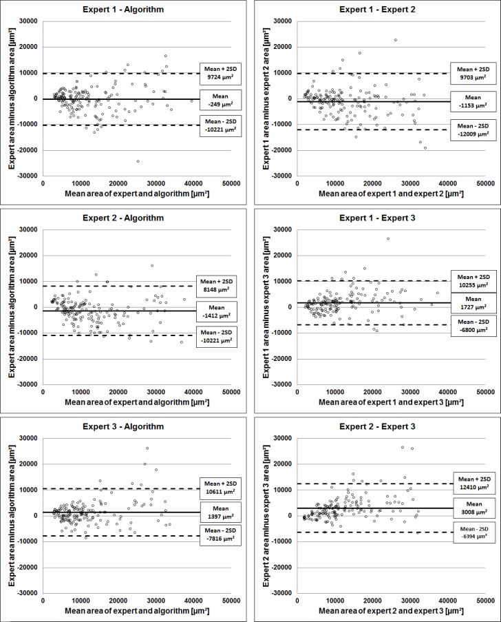
The area deviations of all vessels from the 168 B-scans are shown in a Bland-Altman plot [24] in Fig. 8 in order to compare the inter-reader deviations and the deviations of each expert with the algorithm.
Fig. 8.
Area deviations between the algorithm and the three experts and the inter grader deviations are visualized as Bland-Altman plots.
It can be seen on all plots that as the measurement increases, so does the disagreement, exceeding the standard deviation more likely for larger vessels. The smallest discrepancy between experts and the algorithm is a mean area deviation of −249 ± 9973 µm2 (2×SD) for expert 1, while the biggest discrepancy is a mean area deviation of 1397 ± 9214 µm2 (2×SD) for expert 3. Similarly, the smallest discrepancy among the experts is between expert 1 and expert 2 with a mean area deviation of −1153 ± 10856 µm2 (2×SD), while the biggest discrepancy is between the segmentations of expert 2 and expert 3 with a mean area deviation of 3008 ± 9402 µm2 (2×SD).
The intra reader variability was also tested using the intraclass correlation coefficient (ICC) [25]. The repeated segmentations of 23 blood vessels of 4 different eyes at several time points showed good agreement. An ICC of 0.93 was obtained for the first expert, 0.91 for the second, and 0.94 for the third expert. An ICC between 0.4 and 0.75 is considered fair to good and a higher value excellent agreement.
4. Discussion
In this work we present an algorithm for automatic segmentation of retinal blood vessels in SD-OCT B-scans in lateral and vertical direction. The algorithm uses a model based approach based on a SSM for initial training of blood vessel contours and an ASM application for blood vessel segmentation in unseen images. Compared to the approach for 3-D vessel segmentation based on the graph search [7], retinal surface segmentation is not required. A limitation of our method is that it performs 2-D B-scans rather than 3-D C-scans, as performed in the graph search approach [7]. However, it is possible to segment an entire C-scan by processing the segmentation for each B-scan separately.
We used B-scans from healthy eyes for the verification of our approach, and therefore, the robustness of the proposed algorithm in the context of diseased eyes remains to be demonstrated. Further studies characterizing blood vessels in diseased retinae are underway.
B-scans used in this study were obtained from Spectralis OCT devices and, therefore, are averaged over a defined number of scans in order to reduce speckle noise. Other OCT devices use single B-scans, which may possess a higher speckle noise and can potentially alter detection efficiency. Even though increased noise may therefore be a limitation of the approach, we think that the algorithm performs well under such conditions. The robustness of a SSM for intra-retinal layer segmentation under conditions of increased noise was successfully demonstrated elsewhere [10].
To avoid manual interaction for approximating vessel position prior to segmentation, we implemented a shadowgraph built by the grey-level centers of each A-scan [23]. This feature makes the algorithm fully automatic, which is important for the segmentation of large C-scans and when time is an issue.
The algorithm was validated against manual segmentations on a large set of 168 blood vessels of different sizes from 34 B-scans from 13 healthy eyes done by three different experts. Contour diameter analysis was done between fundus image measurements and B-scan measurements in order to demonstrate proximity of the obtained data to the real anatomical structures. The correlation was always above 0.98. In order to verify the accuracy of vessel boundary segmentation, the mean Euclidean distances of the boundaries were evaluated between the automatic and manual segmentations. Furthermore, the area discrepancy between automatically and manually segmented vessels was tested. The results of the validation indicate that the SSM approach for initial training of the algorithm, and the ASM for segmentation in unseen images, are feasible approaches to obtain accurate segmentations. Overall, the mean Euclidean distances between algorithm and experts are very small in all three situations, approximately 4 pixels resp. 20 µm. The distances among the three experts are approximately 3.8 pixels resp. 18 µm. In the paper proposing the 3D graph search approach [7], only the distances between manually marked blood vessel center points and the automated contour center points were evaluated, rather than comparing entire contour positions, which makes it impossible to compare the accuracy of such an approach with our algorithm.
The evaluation demonstrates that the proposed algorithm is similarly accurate compared to expert readers, and with a very short segmentation time it would be advantageous to use the algorithm in large scale analyses, such as multicenter clinical trials.
Nevertheless, as seen in Fig. 5, even our algorithm is not able to segment the boundaries of every given blood vessel with 100% accuracy. This small discrepancy is due to the limited adaption potential of the ASM, as this is restricted to the available range of trained variations, and local high frequency deformations cannot be fitted exactly by the model. This limitation of automatic segmentation algorithms for locally limited structures is known and cannot be avoided. In any case, the obtained results displayed very high accuracy.
Evaluation of the surface area measurements also revealed a good correlation between automatic segmentation and expert results. The deviations between the algorithm and each of the three experts were not larger than the deviations among the experts themselves. The disagreement among experts and between experts and algorithm increased when the size of the vessel was larger (Fig. 8), which is due to the multiplication of the errors during surface calculation. However, as the aim of the verification method was to demonstrate that the measurements of the algorithm would not differ from expert measurements, this observation is not in disagreement with the general conclusion. This is particularly important, as errors in the surface area measurement would have marked effects on the reliability of the data.
Measurement of blood vessel surfaces is a valuable clinical application, as knowledge about the vessel surface on a B-scan enables further analytical possibilities for the ophthalmologist. For example, the retinal nerve fiber layer (RNFL) can be characterized with or without embedded blood vessels. As large blood vessels make an important part of the RNFL thickness, changes may be better detectable without the presence of the vessels. This algorithm would be a useful tool in the diagnosis of diseases, in which the RNFL thickness may be reduced, such as glaucoma or other optic neuropathies.
In conclusion, the algorithm presented herein is an accurate and reliable tool for the automated segmentation of retinal blood vessels. This enables the ophthalmologist to analyze blood vessels in B- and C-scans and may open the way for new and innovative diagnostic possibilities in the prevention of ocular diseases.
Acknowledgment
The work was supported by a grant from the von Behring Röntgen Foundation (58-0038).
References and links
- 1.Geitzenauer W., Hitzenberger C. K., Schmidt-Erfurth U. M., “Retinal optical coherence tomography: past, present and future perspectives,” Br. J. Ophthalmol. 95(2), 171–177 (2011). 10.1136/bjo.2010.182170 [DOI] [PubMed] [Google Scholar]
- 2.Hoover A., Kouznetsova V., Goldbaum M., “Locating blood vessels in retinal images by piecewise threshold probing of a matched filter response,” IEEE Trans. Med. Imaging 19(3), 203–210 (2000). 10.1109/42.845178 [DOI] [PubMed] [Google Scholar]
- 3.A. Budai, G. Michelson, and J. Hornegger, “Multiscale Blood Vessel Segmentation in Retinal Fundus Images,” in Proceedings of Bildverarbeitung für die Medizin (Springer Verlag, 2010), pp. 261–265. [Google Scholar]
- 4.Sinthanayothin C., Boyce J. F., Cook H. L., Williamson T. H., “Automated localisation of the optic disc, fovea, and retinal blood vessels from digital colour fundus images,” Br. J. Ophthalmol. 83(8), 902–910 (1999). 10.1136/bjo.83.8.902 [DOI] [PMC free article] [PubMed] [Google Scholar]
- 5.Niemeijer M., Garvin M. K., van Ginneken B., Sonka M., Abràmoff M. D., “Vessel segmentation in 3D spectral OCT scans of the retina,” Proc. SPIE 6914, 69141R–, 69141R-8. (2008). 10.1117/12.772680 [DOI] [Google Scholar]
- 6.J. Xu, D. Tolliver, H. Ishikawa, C. Wollstein, and J. Schuman, “Blood vessel segmentation with three-dimensional spectral domain optical coherence tomography,” International Patent no. WO/2010/138645 (Feb. 12, 2010).
- 7.K. Lee, “Segmentations of the intraretinal surfaces, optic disc and retinal blood vessels in 3D-OCT scans,” Ph.D. dissertation (University of Iowa, 2009), pp. 57–69. [Google Scholar]
- 8.Fernández D. C., “Delineating fluid-filled region boundaries in optical coherence tomography images of the retina,” IEEE Trans. Med. Imaging 24(8), 929–945 (2005). 10.1109/TMI.2005.848655 [DOI] [PubMed] [Google Scholar]
- 9.Perona P., Malik J., “Scale-space and edge detection using anisotropic diffusion,” IEEE Trans. Pattern Anal. Mach. Intell. 12(7), 629–639 (1990). 10.1109/34.56205 [DOI] [Google Scholar]
- 10.Kajić V., Považay B., Hermann B., Hofer B., Marshall D., Rosin P. L., Drexler W., “Robust segmentation of intraretinal layers in the normal human fovea using a novel statistical model based on texture and shape analysis,” Opt. Express 18(14), 14730–14744 (2010). 10.1364/OE.18.014730 [DOI] [PubMed] [Google Scholar]
- 11.Selesnick I. W., Baraniuk R. G., Kingsbury N. G., “The dual-tree complex wavelet transform,” IEEE Signal Process. Mag. 22(6), 123–151 (2005). 10.1109/MSP.2005.1550194 [DOI] [Google Scholar]
- 12.Wong A., Mishra A., Bizheva K., Clausi D. A., “General Bayesian estimation for speckle noise reduction in optical coherence tomography retinal imagery,” Opt. Express 18(8), 8338–8352 (2010). 10.1364/OE.18.008338 [DOI] [PubMed] [Google Scholar]
- 13.Cootes T., Taylor C., Cooper D., Graham J., “Active shape models—their training and application,” Comput. Vis. Image Underst. 61(1), 38–59 (1995). 10.1006/cviu.1995.1004 [DOI] [Google Scholar]
- 14.T. Cootes, C. Taylor, A. Lanitis, D. Cooper, and J. Graham, “Building and using flexible models incorporating grey-level information,” in Fourth International Conference on Computer Vision, 1993. Proceedings (1993), pp. 242–246. [Google Scholar]
- 15.Kelemen A., Székely G., Gerig G., “Elastic model-based segmentation of 3-D neuroradiological data sets,” IEEE Trans. Med. Imaging 18(10), 828–839 (1999). 10.1109/42.811260 [DOI] [PubMed] [Google Scholar]
- 16.Lamecker H., Seebaß M., Hege H.-C., Deuflhard P., “A 3D statistical shape model of the pelvic bone for segmentation,” Proc. SPIE 5370, 1341–1351 (2004). 10.1117/12.534145 [DOI] [Google Scholar]
- 17.J. Hug, C. Brechbühler, and G. Székely, “Model-based Initialisation for Segmentation,” in Computer Vision—ECCV 2000 (Springer, 2000), pp. 290–306. [Google Scholar]
- 18.G. Edwards, T. Cootes, and C. Taylor, “Advances in active appearance models,” The Proceedings of the Seventh IEEE International Conference on Computer Vision (IEEE, 1999), Vol. 1, pp. 137–142. [Google Scholar]
- 19.R. Fisker, N. Schultz, N. Duta, and J. Carstensen, “A general scheme for training and optimization of the Grenander deformable template model,” in IEEE Conference on Computer Vision and Pattern Recognition,2000. Proceedings (IEEE, 2000), pp. 698–705. [Google Scholar]
- 20.M. Stegmann, R. Fisker, and B. Ersbøll, “Extending and applying active appearance models for automated, high precision segmentation in different image modalities,” in Scandinavian Conference on Image Analysis, (2001), pp. 90–97. [Google Scholar]
- 21.D. Goldberg, Genetic Algorithms in Search, Optimization, and Machine Learning (Addison-Wesley, Bonn, 1989). [Google Scholar]
- 22.Hill A., Taylor C., “Model-based image interpretation using genetic algorithms,” Image Vis. Comput. 10(5), 295–300 (1992). 10.1016/0262-8856(92)90045-5 [DOI] [Google Scholar]
- 23.Wehbe H., Ruggeri M., Jiao S., Gregori G., Puliafito C. A., Zhao W., “Automatic retinal blood flow calculation using spectral domain optical coherence tomography,” Opt. Express 15(23), 15193–15206 (2007). 10.1364/OE.15.015193 [DOI] [PubMed] [Google Scholar]
- 24.Bland J. M., Altman D. G., “Statistical methods for assessing agreement between two methods of clinical measurement,” Lancet 327(8476), 307–310 (1986). 10.1016/S0140-6736(86)90837-8 [DOI] [PubMed] [Google Scholar]
- 25.H. Fleiss, Statistical Methods for Rates and Proportions, 2nd ed. (Wiley New York, 1981). [Google Scholar]


