Abstract
Purpose: This work is to provide a direct, quantitative comparison of image features measured by film and full-field digital mammography (FFDM). The purpose is to investigate whether there is any systematic difference between film and FFDM in terms of quantitative image features and their influence on the performance of a computer-aided diagnosis (CAD) system.
Methods: The authors make use of a set of matched film-FFDM image pairs acquired from cadaver breast specimens with simulated microcalcifications consisting of bone and teeth fragments using both a GE digital mammography system and a screen-film system. To quantify the image features, the authors consider a set of 12 textural features of lesion regions and six image features of individual microcalcifications (MCs). The authors first conduct a direct comparison on these quantitative features extracted from film and FFDM images. The authors then study the performance of a CAD classifier for discriminating between MCs and false positives (FPs) when the classifier is trained on images of different types (film, FFDM, or both).
Results: For all the features considered, the quantitative results show a high degree of correlation between features extracted from film and FFDM, with the correlation coefficients ranging from 0.7326 to 0.9602 for the different features. Based on a Fisher sign rank test, there was no significant difference observed between the features extracted from film and those from FFDM. For both MC detection and discrimination of FPs from MCs, FFDM had a slight but statistically significant advantage in performance; however, when the classifiers were trained on different types of images (acquired with FFDM or SFM) for discriminating MCs from FPs, there was little difference.
Conclusions: The results indicate good agreement between film and FFDM in quantitative image features. While FFDM images provide better detection performance in MCs, FFDM and film images may be interchangeable for the purposes of training CAD algorithms, and a single CAD algorithm may be applied to either type of images.
Keywords: full-field digital mammography (FFDM), screen-film mammography, clustered microcalcifications, textural features, computer-aided diagnosis (CAD)
INTRODUCTION
Mammography is currently the standard clinical tool for breast cancer screening. With the introduction of full-field digital mammography (FFDM), there have been recent studies comparing FFDM images with traditional film mammograms. These two types of mammograms, i.e., screen-film vs FFDM, have advantages and limitations on certain aspects, related or unrelated to the diagnostic accuracy of breast cancer.1 The digital mammographic imaging screening trial (DMIST) (Ref. 2) showed that radiologists’ screening performance using FFDM is similar to that obtained using screen-film mammography (SFM); however, FFDM was superior when imaging women with dense breasts.
There has been interest in comparing the effects of film and digital mammograms on computer-aided diagnosis (CAD). For example, in the study of Rana et al. the diagnostic performance of existing CAD algorithms, developed based on film mammograms, was investigated when applied to FFDM images.3 It was demonstrated that similar results could be obtained by FFDM mammograms, suggesting that CAD algorithms developed using film mammograms can be applied to FFDM mammograms without substantial modification. Also, Boone et al. showed that FFDM images tend to have higher signal-to-noise ratio than film images for the same x-ray exposure.4
In this work, we conduct a direct, quantitative comparison of image features measured by film and FFDM images acquired from same breast specimens. The goal is to investigate in a controlled manner whether the two types of images yield comparable image features for use in CAD algorithms. It should be noted that this is quite different from previous comparison studies, such as that of Rana et al., wherein the diagnosis performance was compared across different datasets.3
The use of cadaveric specimens is well suited for our purposes, since it permits comparable images to be acquired on screen-film and FFDM systems, thereby allowing meaningful quantitative comparisons. In addition, it permits multiple images to be acquired, which is not usually possible for live subjects. There is ample precedent for this approach: mastectomy specimens and cadaveric breasts have been used in numerous studies to achieve anatomically realistic backgrounds,4, 5, 6, 7, 8 and are particularly useful for comparisons between imaging systems. While it is possible to obtain FFDM and SFM on the same patient, the two images are not comparable. It is impossible to position and compress a breast in the exact same manner on both systems (with the possible exception of CR mammograms). Therefore, a distinctive advantage of using cadaver breasts over using multiple mammograms of same subjects is that it allows for image acquisition of the breast tissue in the same position and compression between film and FFDM.
The motivation for our study is to determine whether image features derived from film and FFDM are significantly different from one another to warrant that they be treated separately when developing CAD algorithms. CAD development requires the availability of a large database of mammograms; thus, it would be desirable to utilize existing data sets of both film and FFDM if it can be demonstrated that the features derived from these two types of images are interchangeable. This would greatly increase the amount of data available to CAD systems.
We used pairs of images (acquired using film and FFDM) to compare feature values obtained from these two types of images; the features considered are ones that have been previously used in CAD to characterize microcalcifications.9 We compared the paired feature values, and also studied the performance of CAD algorithms derived using these values. In particular, we consider both a CAD detection algorithm and a CAD classification algorithm for discriminating against false positives; for the latter, we investigate how the performance of the CAD classifier will be affected when it is trained on one type of images but tested on a different type.
In this study, we focus on analyzing images containing microcalcification (MC) lesions. MCs are tiny calcium deposits which appear as bright spots in mammograms. Clustered MCs can be an important early sign of breast cancer, appearing in 30%–50% of mammographically diagnosed cases.10 In the literature, there has been significant interest in the development of CAD algorithms for detection and classification of MC lesions.
The rest of the paper is organized as follows. A description of the image dataset and quantitative image features used in this study is given in Sec. 2, followed in Sec. 3 by a comparison study on how the image features from film or FFDM images may affect the performance of CAD algorithms. Experimental results on image feature values and performance of CAD algorithms are furnished in Sec. 4, and conclusions are drawn in Sec. 5.
QUANTITATIVE COMPARISON OF IMAGE FEATURES
In this section, we focus on direct comparison of quantitative image features extracted from film and FFDM images of the same specimens. In particular, we consider two broad types of quantitative image features: (1) image textural features, and (2) microcalcification image features, both of which have been commonly used in the literature for detection and classification of MC lesions in CAD algorithms.11, 12
Description of dataset acquisition
We make use of a set of images of anonymized cadaveric breast specimens obtained from the University of Chicago Anatomical Gift Association. Each specimen was fixed in a Lucite container and immersed in water. The x-ray attenuation coefficient of water is similar to that of breast tissue, and was used to minimize the radiographic appearance of macroscopic skin wrinkles. Simulated MCs consisting of bone and tooth fragments with a range of sizes from 100 to 1000 μm (on their long axes) were fixed in glass dishes, and were overlaid on the breast specimens. The cadaver breasts overlaying the simulated calcifications were imaged at 31 kVp with Mo anode and a Rh filter. Using the automatic exposure control, images were made on the screen-film system. The same exposure conditions were used on the FFDM system.
The FFDM images were acquired using a Senographe 2000D FFDM system (General Electric Medical Systems; Milwaukee, WI), with a resolution of 100 μm per pixel and each pixel was represented using 14 bits. We used the for-processing images. The film images were acquired using a Min-R 2000 screen-film system (Eastman Kodak, Rochester, NY) on a DMR mammography system (General Electric Medical Systems; Milwaukee, WI). They were scanned on a Lumiscan film digitizer (Lumisys; Sunnyvale, CA), which produced images with spatial and gray-scale resolution of 50 μm and 12-bit, respectively. These were down sampled to 100 μm to match the FFDM images.
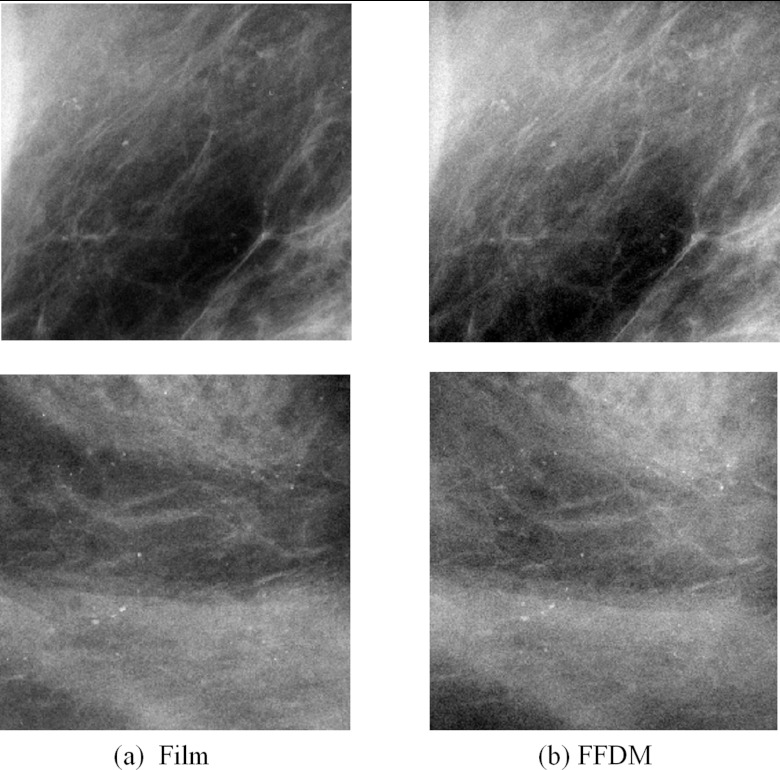
Figure 1 shows regions of interest (ROIs) in two example pairs of film and FFDM images, illustrating the relatively subtle visual differences between film and FFDM. For quantitative comparison in this study, we extracted 20 matched pairs of film and FFDM ROIs, each with dimension of 512 × 512 pixels. These ROIs were from cadaver breasts of five different female subjects (four ROIs from each subject, all with different simulated MC clusters) and they were spatially nonoverlapping.
Figure 1.
Two film-FFDM image pairs, in which bone and tooth fragments with a range of sizes from 100 and 1000 μm were used to simulated MCs.
Quantification of textural features
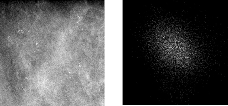
To obtain textural features for each image, we use the method of spatial gray level dependence (SGLD) matrices,13 a method that has found many applications in medical image analysis, including characterizing tissue regions containing clustered MCs in mammograms.9 For a given image, a SGLD matrix (also known as a co-occurrence matrix) is formed by the joint distribution of the gray levels at two pixels that are separated by a specified distance along a fixed orientation. By varying both the separation distance and orientation parameters, one can obtain a set of SGLD matrices. As an example, we show in Fig. 2 the SGLD matrix of a sample FFDM mammogram ROI obtained when the distance and direction parameters were 16 pixels and 0°, respectively.
Figure 2.
A FFDM mammogram ROI (left) and its corresponding SGLD matrix (right).
From the SGLD matrices, we calculate a set of 12 textural features: (1) energy (ENER), (2) entropy (ENTR), (3) difference average (DFAV), (4) difference variance (DFVR), (5) difference entropy (DFEN), (6) sum average (SMAV), (7) sum variance (SMVR), (8) sum entropy (SMEN), (9) inverse difference moment (INVD), (10) correlation (COR), (11) and (12) information measures of correlation (ICO1, ICO2). A detailed definition of these textural features is given in the Appendix. These textural features are used to characterize image properties related to transition of gray levels in an image. For example, the entropy measures the uniformity of the SGLD matrix. A large entropy value implies a more uniform SGLD matrix and correspondingly more random variations in gray-level pairs in the image. The features related to the sum (or difference) are used to characterize the distribution of the sum (or difference) of the gray-level pairs in the image. These features were demonstrated previously to be salient for classifying MC lesions.9
Prior to calculation of these features, a background correction step was first applied to the images to remove the effect of nonuniform tissue background.9 Afterward, all images were normalized to have zero mean and unit variance. Then the resulting images were quantized to the same number of gray levels and the SGLD matrices were formed, from which the above textural features were calculated. Note that the normalization step was to ensure that the same quantization was applied to the different images, so that the extracted texture features would be invariant to scaling in image intensity. This is because the texture patterns in an image remain the same when the intensity of the image is adjusted in a linear proportion.
Quantification of MC image features
Besides textural features, we also characterized the individual MCs by using a set of six features that have been used previously to detect and classify clustered MCs:11, 14, 15 (1) area (or size) of a MC, measured by the number of pixels, (2) mean image intensity value of the pixels of a MC, (3) standard deviation of the image intensity values among the MC pixels, (4) image contrast, computed as the difference between the mean intensity value of the MC and its surrounding background, (5) the effective volume of the MC (area times effective thickness), and (6) shape irregularity, measured by the variance of the distance from MC boundary to its geometric center.14
Prior to extraction of these features, the individual MCs in the images were first segmented out using a local threshold method.16 For each MC the segmentation threshold was set as T = μ + c × σ, where μ and σ denote the local mean and standard deviation, respectively, which were estimated from a 101 × 101-pixel region centered around the MC, and the coefficient c was set to 3. From the 20 ROIs, we extracted the aforementioned six features for a total of 495 individual MCs.
COMPARISON OF IMAGE FEATURES IN CAD ALGORITHMS
In this section, we investigate how choice of film or FFDM may affect the performance of CAD algorithms. In particular, we first study whether these two types of images would yield the same level of detection accuracy when a CAD algorithm is applied for MC detection. We then investigate how the performance of a CAD classifier would be affected when it is trained on features extracted from one type of images but applied to images of a different type; the task of this classifier is to discriminate true positives from false positives in the context of MC detection.
Detectability of microcalcifications
In this study, the locations of the MCs in the test specimens were known exactly, allowing us to measure and compare the detectability of the MCs in the two types of images. To perform the MC detection, we applied the difference of Gaussian (DoG) detector which was previously described in the literature.16, 17 While there exist other more sophisticated methods for MC detection in the literature, we chose the DoG detector in this study in favor of its simplicity because it does not require retraining. The DoG detector consists of two Gaussian kernels of different width parameters, which were set to σ1 = 1.1 and σ2 = 1.4.16
For MC detection in each image, the DoG output was first compared to an operating threshold; the surviving pixels that were adjacent to each other were grouped to form MC objects. To reduce the number of false positives (FPs), detected objects smaller than 3 pixels were discarded as spurious detections. Afterward, the detection performance was computed for each type of images (film or FFDM) using free-response receiver operating characteristic (FROC) curves,18 which plot the fraction of correct detections of MC objects (i.e., true positive fraction (TPF)) versus the average number of FPs per image, over the continuum of values for the operating threshold.
Saliency of MC image features in CAD algorithms
In this section, we investigate whether film and FFDM are interchangeable when training a CAD system. Specifically, when the task is to discriminate MC objects from FPs, we seek to determine whether different results are obtained when film images, FFDM images, or a mixture of both types are used for training.
Our experiments consisted of the following steps. First, a set of data examples of both MC objects and non-MC objects (i.e., FPs) was extracted from all the film images (as described later in detail), and the six image features in Sec. 2C were extracted for each of these examples; this set of examples will subsequently be denoted by S1. Next, a set of MC and non-MC examples was similarly obtained from the FFDM images, denoted by S2. Afterward, these two sets of examples were used to compare the classifier performance across different choices of the image types used in training and testing, as further explained later.
To determine whether the classifier performance is affected by the choice of the image type used for training (film or FFDM), we tested and compared classifiers trained using the following sources of training images: (1) film examples (S1) only, (2) FFDM examples (S2) only, and (3) mixture of film and FFDM samples (equal number of samples selected randomly from S1 and S2).
The film examples in S1 were obtained as follows. First, all the known 495 MC objects were extracted from the images as MC-class examples. Afterward, an equal number of non-MC class examples were extracted from these images; these non-MC examples were randomly selected from the FPs generated by the DoG detector in these images. The operating threshold of the DoG was set as at a level such that the average number of FPs would be about 5 times the number of true MCs in each image, the purpose being to ensure the detection rate to be above 90% for true MCs. The FFDM samples in S2 were similarly obtained.
A support vector machine (SVM) classifier with Gaussian radial basis function (RBF) kernel was used to classify the MC and FP samples.19 The kernel width parameter σ and the penalty parameter C were determined during training. To evaluate the classifier performance, we applied a fivefold cross validation procedure in which all the examples were randomly partitioned into five equal-sized subsets. Each of these subsets was held out in turn for testing, with the rest being used to train the classifier. Afterward, the classifier output was analyzed by the ROCKIT software,20 and the performance was summarized using ROC curves.
It should be noted that the MC examples from film and FFDM images have near-perfect correspondence in terms of their locations, while non-MC examples have no accurate correspondence, since they consist of mostly noise. For purpose of fair cross validation as described earlier, we built a correspondence map for non-MC examples based on their distance from each other, i.e., for each non-MC example in a film image, its corresponding non-MC example from FFDM image was identified as the one with smallest Euclidean distance from it. The purpose is to make sure that samples from a film image are not used to train a classifier that will be tested on their corresponding samples from a FFDM image if they are too close to each other.
RESULTS AND DISCUSSIONS
Quantification of textural features
In Table 1 we show statistics (mean and variance) and comparison results (correlation coefficients and p-values) for the 12 textural features described in Sec. 2B obtained from the 20 film-FFDM image pairs. The Pearson's correlation coefficient, which measures concordance between the feature values obtained from film and FFDM, ranges from 0.8303 to 0.9602 for the 12 textural features. When these features are considered together as a vector for each image (after standardizing each feature to have zero mean and unit variance so that the correlation coefficient will be not dominated by those features with exceedingly large values), the correlation coefficient between the film and FFDM is 0.8877. There is indeed a high degree of agreement between the textural features extracted from film and FFDM image pairs.
Table 1.
Comparison between film and FFDM for 12 textural features.
| Film value | FFDM value | |||
|---|---|---|---|---|
| Features | (std. dev.) | (std. dev.) | Corr. coeff. | p-value |
| DFAV | 21.88 (4.431) | 21.69 (4.458) | 0.9190 | 1.0000 |
| DFVR | 329.2 (123.7) | 321.0 (126.3) | 0.9602 | 1.0000 |
| DFEN | 5.809 (0.3456) | 5.797 (0.3486) | 0.9057 | 1.0000 |
| SMAV | 256.8 (3.648) | 256.8 (3.063) | 0.8338 | 0.8238 |
| SMVR | 1706 (257.2) | 1731 (216.5) | 0.8773 | 1.0000 |
| SMEN | 7.320 (0.1115) | 7.335 (0.0930) | 0.8568 | 0.5034 |
| INVD | 0.0487 (0.0149) | 0.0494 (0.0127) | 0.8801 | 0.5034 |
| ENER | 0.0003 (0.0001) | 0.0003 (0.0001) | 0.8910 | 0.5034 |
| ENTR | 12.04 (0.2924) | 12.05 (0.2857) | 0.9008 | 0.5034 |
| COR | 0.3790 (0.2357) | 0.4035 (0.2364) | 0.9435 | 0.2632 |
| ICO1 | 0.1743 (.0264) | 0.1753 (0.0235) | 0.8303 | 0.8238 |
| ICO2 | 0.9468 (.0186) | 0.9480 (0.0158) | 0.8534 | 0.8238 |
As a further comparison of feature values derived from film and FFDM, we applied Fisher sign test to the feature pairs.21 The Fisher sign test is a nonparametric approach that is robust to the underlying distributions. The results in Table 1 show that all p-values exceed the significance level of 0.05 for all 12 features (the smallest p-value being 0.2632). Thus, no statistically significant difference was observed between the features derived from film and that derived from FFDM. We caution that the above comparison was based on only 20 samples, which did not show statistical significance between SFM and FFDM features.
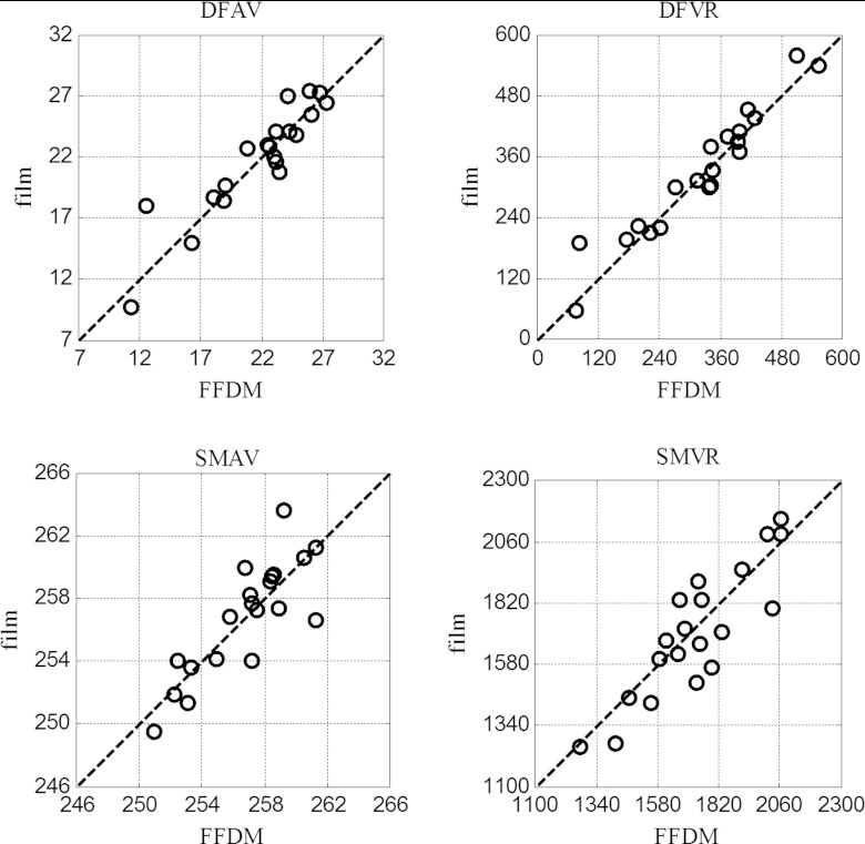
In Fig. 3 we show the scatter plots of the feature values of the film-FFDM image pairs for the following four textural features: DFAV, DFVR, SMAV, and SMVR; in these plots, each data point represents the feature values from a particular film-FFDM image pair. Note that in the ideal case of a perfect match between film and FFDM, all the data points would fall precisely on the 45° line. Similar plots were also obtained for the other eight textural features, but since they look essentially similar, they are not shown here. Collectively, these results suggest strong agreement between the film and FFDM feature values.
Figure 3.
Comparison of film vs FFDM for four example textural features for lesion region in the 20 ROIs.
In the above results the following parameters were used for calculating the SGLD matrices: 8-bit quantization intervals were used, and the distance and direction parameters were set to 16 pixels and 0°, respectively. We also tested with other parametric settings, and similar results were obtained.
Quantification of MC image features
In Table 2 we summarize results obtained on the six MC image features described in Sec. 2C, namely, (1) MC size (AREA), (2) mean image intensity value of the MC pixels (INTAV), (3) standard deviation of the image intensity value among the MC pixels (INTSD), (4) MC image contrast (CONT), (5) effective volume of the MC (VOLU), and (6) shape irregularity (SHAPE). These results were obtained from all the 495 MCs in the 20 film-FFDM image pairs, from which the mean and standard deviation were computed for each feature.
Table 2.
Comparison between film and FFDM for six image features of MCs.
| Film value | FFDM value | |||
|---|---|---|---|---|
| Features | (std. dev.) | (std. dev.) | Corr. coef. | p-value |
| AREA | 0.1349 (0.0706) | 0.1370 (0.0701) | 0.8909 | 0.3676 |
| INTAV | 1.392 (1.027) | 1.398 (1.049) | 0.8643 | 0.4930 |
| INTSD | 0.3630 (0.2105) | 0.3720 (0.1997) | 0.7448 | 0.1417 |
| CONT | 1.105 (0.5898) | 1.058 (0.5545) | 0.8812 | 0.2813 |
| VOLU | 17.01 (17.32) | 16.64 (17.19) | 0.9269 | 0.3781 |
| SHAPE | 1.030 (0.2483) | 1.047 (0.6551) | 0.7326 | 0.6244 |
Table 2 shows the correlation coefficients between MC features derived from the film and FFDM images, ranging from 0.7326 to 0.9269. When these features are considered together as a vector for each MC, the correlation coefficient between the film and FFDM is 0.8236. Similar to the textural features, there is considerable agreement between film and FFDM. We also applied a Fisher sign test to the six MC features, yielding no significant difference between the film and FFDM distributions (p-values ranged from 0.1417 to 0.6244, all greater than the significance level of 0.05).
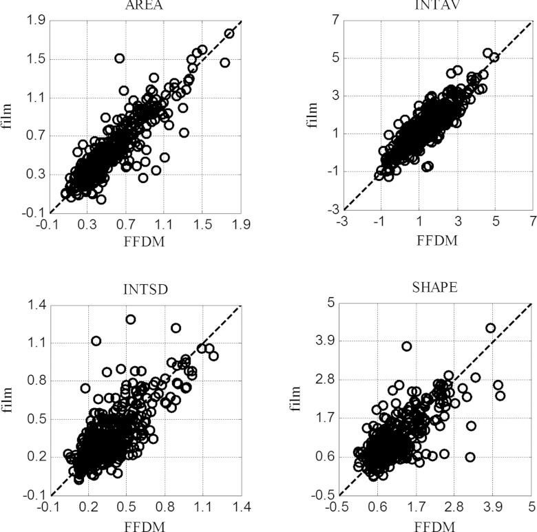
In Fig. 4 we show the scatter plots for the AREA, INTAV, INTSD, and SHAPE features. In these plots, each data point represents the feature values of a particular MC in the film-FFDM image pairs. Similar plots were also obtained for the other two MC features, but not shown here for the sake of brevity.
Figure 4.
Comparison of film vs FFDM for four image features obtained from 495 MCs.
By comparing with the results earlier in Sec. 4A, it is noted that the agreement between film and FFDM is generally higher for the textural features than for the MC features. This is likely caused by the fact that the textural features were computed from the entire image region, while the MC features were computed from individual MC objects which were much smaller in size. The latter features would become more sensitive to the image noise due to fewer pixels for averaging. This in particular is reflected by the results for the SHAPE feature, which has the smallest correlation coefficient among the six MC features; the shape of a small MC object can be easily affected by the noise even when only one or two pixels are incorrectly segmented.
Comparison of MC detectability
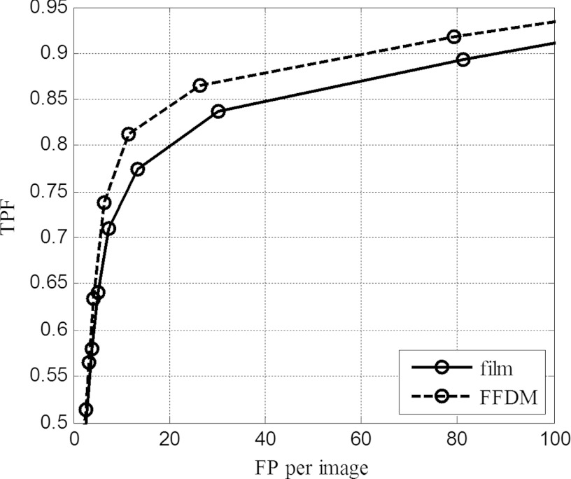
The MC detection results of film and FFDM images by the DoG detector are summarized using FROC curves in Fig. 5. In this plot, the abscissa is the average number of FP detections per image, and the ordinate is the detection rate of the MCs. Thus, a higher FROC curve indicates better detection by a detector. The figure shows that better detection is obtained when the detector is applied to the FFDM images than to the film images. For example, with the false detection level at 20 FP signals per image, the MC detection rate is around 85% for FFDM, compared to about 80% for film. A p-value of 0.0260 was obtained for comparison of the FROC curves using a bootstrapping method,22 which implies a significant difference between the detection performance by the DoG detector on this set of film and FFDM images. This is likely a result of higher image quality (less noisy) in FFDM, as reported in other studies in the literature.23, 24 For example, it was reported that MC detection in patients was better on FFDM for two of the three human observers.23 Equivalent or better MC detection by FFDM was also reported in phantom studies.25, 26 Our results in Fig. 5 using matched film-FFDM image pairs are consistent with findings from these reported studies.
Figure 5.
FROC curves obtained from film and FFDM obtained with DoG detector.
Comparison of saliency of MC features
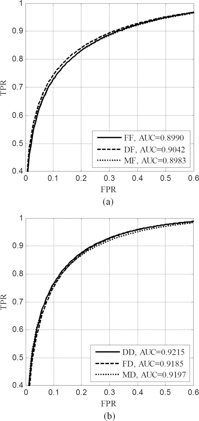
In Fig. 6a we show the classification results obtained by the SVM classifier on the set of MC and non-MC samples in S1 (film images). For comparison, the resulting ROC curves are shown when the classifier was trained with each of the following: (1) film examples S1 (FF), (2) FFDM examples S2 (DF), and (3) a mixture of film and FFDM examples (MF); the corresponding area under the ROC curve (AUC) for these three cases was found to be 0.8990 (std. = 0.0102), 0.9042 (std. = 0.0102), and 0.8983 (std. = 0.0103), respectively. The p-value from a statistical comparison between FF and DF was 0.2782, and the p-value between FF and MF was 0.6422. These results indicate that the classification performance on the film images does not depend substantially on whether the classifier was trained with film images, FFDM images, or a mixture of the two image types.
Figure 6.
Classification performance for discrimination of MC from false-positives in different images: (a) film and (b) FFDM. In each case, the classifier was trained with different types of images.
Similarly, in Fig. 6b we show the classification results obtained by the SVM classifier on the set of MC and non-MC samples in S2, which was from FFDM images; the classifier was trained on each of the three types of samples, i.e., film samples S1, FFDM samples S2, or their mixture. The corresponding area under the ROC curve was 0.9215 (std. = 0.0094), 0.9185 (std. = 0.0096), and 0.9197 (std. = 0.0094), respectively. The p-value from a statistical comparison between DD and FD was 0.1814, and the p-value between DD and MD was 0.1514. Similar to the results on film images above, there was no significant difference in the classification performance when the classifier was trained with different types of images.
Furthermore, comparing the results in Fig. 6a with those in Fig. 6b, it is noteworthy that the overall classification performance is higher when the classifier is applied to FFDM images than to film images, with the average AUC = 0.9199 for FFDM and 0.9005 for film. The p-value from a statistical comparison between the two was 0.0134. (It should be noted that the non-MC samples from film and FFDM images have only loose correspondence.) This indicates that the classifier can better separate MCs from FPs in FFDM images than in film images. This is likely due to the higher image quality in FFDM. Interestingly, this is also consistent with the better detection performance for MCs in FFDM images observed in Sec. 4C.
Further discussions
The classification results for film and FFDM examples in Sec. 4D show slightly better classification performance for FFDM images; however, the performance of the classifier is observed to be relatively unaffected by the choice of image types used for training. This is intriguing, as it may indicate that, while there might be some difference in image quality between film and FFDM, the extracted image features might be interchangeable when training a CAD system.
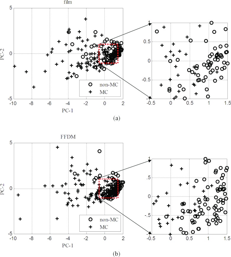
To better understand this, we further investigated the distribution of the MC image features for both film and FFDM by using principal component analysis (PCA). In Fig. 7a, we show a scatter plot of the first two PCA components of the feature vectors of the film examples S1, where the MC and non-MC samples are indicated with different symbols; for clarity in the graph, only 100 samples randomly selected from each class are shown. Similarly, in Fig. 7b, we show a scatter plot for the FFDM examples S2.
Figure 7.
PCA plot for MC and non-MC samples from different types of images: (a) film and (b) FFDM.
From Fig. 7 it can be observed that the film and FFDM features show similar distributions in the scatter plots. This is consistent with the results in Sec. 4B, where good agreement was observed between film and FFDM in terms of individual features of MC. However, the scatter plots also reveal that there is slightly better separation between MC and non-MC samples in FFDM than in film. Indeed, we computed the Fisher discriminant ratio (FDR) between the two classes in the PCA plots in Fig. 7. The obtained FDR values are 1.99 and 2.15 for film and FFDM, respectively, indicating a higher degree of separability in FFDM. Interestingly, this is consistent with the better classification performance in FFDM observed in Fig. 6. The plot in Fig. 7a shows more overlap between non-MC and MC samples; such confusion is likely caused by the higher noise in film. This is also consistent with the higher detection performance in FFDM observed in Fig. 5.
CONCLUSIONS
In this work, we conducted a comparison study of image features measured by film and FFDM. By making use of a set of matched film-FFDM image pairs acquired from cadaveric breast specimens, we were able to provide a meaningful comparison of the two types of images in terms of both their quantitative image features and their influence on CAD algorithms. The image features considered include textural features of lesion regions and image features of individual MCs, both of which have been used in CAD algorithms for breast lesions. The results show that there is a great degree of agreement in the image features measured from film and FFDM images, and no significant difference was observed between them. Furthermore, the results also show that there is little difference in the classification performance of a CAD classifier when it is trained with image features extracted from film or FFDM images or even a mixture of them. However, better detection performance for MCs was observed when the algorithm is applied to the FFDM images than to the film images, which is likely attributed to the better image quality (lower noise) in FFDM. These results indicate that film and FFDM images may be used interchangeably in training a CAD system without sacrificing performance. However, in consideration of the specific imaging systems, limited number of images, features and specific algorithms investigated in this work, the consistency between film and FFDM features should be examined with caution given the complexity of real CAD systems.
ACKNOWLEDGMENT
This work was supported in part by NIH/NIBIB (Grant No. R01EB009905).
APPENDIX: TEXTURAL FEATURES USED IN THIS STUDY
Let p(i, j) denote the (i, j) th element in a SGLD matrix. Then these 12 features are derived from p(i, j) as follows:
| (A1) |
| (A2) |
| (A3) |
| (A4) |
| (A5) |
| (A6) |
| (A7) |
| (A8) |
| (A9) |
| (A10) |
| (A11) |
| (A12) |
In the above definitions, is the marginal probability of the ith entry over x, μx, and σx are its associated mean and standard deviation, HX is its entropy, and Ng is the number of gray levels. Furthermore,
| (A13) |
| (A14) |
| (A15) |
| (A16) |
| (A17) |
References
- Tice J. and Feldman M., “Full-field digital mammography compared with screen-film mammography in the detection of breast cancer: Rays of light through DMIST or more fog,” Breast Cancer Res. Treat. 107, 157–165 (2008). 10.1007/s10549-007-9545-4 [DOI] [PubMed] [Google Scholar]
- Pisano E. et al. , “Diagnostic performance of digital versus film mammography for breast-cancer screening,” N. Eng. J. Med. 353, 1773–1783 (2005). 10.1056/NEJMoa052911 [DOI] [PubMed] [Google Scholar]
- Rana R. et al. , “Independent evaluation of computer classification of malignant and benign calcifications in full-field digital mammograms,” Acad. Radiol. 14, 363–370 (2007). 10.1016/j.acra.2006.12.012 [DOI] [PMC free article] [PubMed] [Google Scholar]
- Boone J. et al. , “Dedicated breast CT: Radiation dose and image quality evaluation,” Radiology 221, 657–667 (2001). 10.1148/radiol.2213010334 [DOI] [PubMed] [Google Scholar]
- Niklason L. and Christian B. et al. , “Digital tomosynthesis in breast imaging,” Radiology 205, 399–406 (1997). [DOI] [PubMed] [Google Scholar]
- Suryanarayanan S. et al. , “Comparison of tomosynthesis methods used with digital mammography,” Acad. Radiol. 7, 1085–1097 (2000). 10.1016/S1076-6332(00)80061-6 [DOI] [PubMed] [Google Scholar]
- KimmeSmith C. et al. , “Mammography fixed grid versus reciprocating grid: Evaluation using cadaveric breasts as test objects,” Med. Phys. 23, 141–147 (1996). 10.1118/1.597695 [DOI] [PubMed] [Google Scholar]
- Shepherd J. et al. , “Measurement of breast density with dual x-ray absorptiometry: Feasibility,” Radiology 223, 554–557 (2002). 10.1148/radiol.2232010482 [DOI] [PubMed] [Google Scholar]
- Chan H. et al. , “Computerized analysis of mammographic microcalcifications in morphological and texture feature space,” Med. Phys. 25, 2007–2019 (1998). 10.1118/1.598389 [DOI] [PubMed] [Google Scholar]
- American Cancer Society, Cancer Facts and Figures 2009 (American Cancer Society (ACS), Atlanta, GA, 2009). [Google Scholar]
- Elter M. and Horsch A., “CADx of mammographic masses and clustered microcalcifications: A review,” Med. Phys. 36, 2052–2068 (2009). 10.1118/1.3121511 [DOI] [PubMed] [Google Scholar]
- Soltanian-Zadeh H., Rafiee-Rad F., and Pourabdollah-Nejad S., “Comparison of multiwavelet, wavelet, Haralick, and shape features for microcalcification classification in mammograms,” Pattern Recogn. 37, 1973–1986 (2004). 10.1016/j.patcog.2003.03.001 [DOI] [Google Scholar]
- Haralick R., Shanmugam K., and Dinstein I., “Textural features for image classification,” IEEE Trans. Syst. Man Cybern. 3, 610–621 (1973). 10.1109/TSMC.1973.4309314 [DOI] [Google Scholar]
- Jiang Y., Nishikawa R. M., Wolverton E. E., Metz C. E., Giger M. L., Schmidt R. A., and Vyborny C. J., “Malignant and benign clustered microcalcifications: Automated feature analysis and classification,” Radiology 198, 671–678 (1996). [DOI] [PubMed] [Google Scholar]
- Rangayyan R., Fabio J., and Desautels J., “A review of computer-aided diagnosis of breast cancer: Toward the detection of subtle signs,” J. Franklin Inst. 344, 312–348 (2007). 10.1016/j.jfranklin.2006.09.003 [DOI] [Google Scholar]
- Salfity M., Nishikawa R., Jiang Y., and Papaioannou J., “The use of a priori information in the detection of mammographic microcalcifications to improve their classification,” Med. Phys. 30, 823–831 (2003). 10.1118/1.1559884 [DOI] [PubMed] [Google Scholar]
- Dengler J., Benrens S., and Desaga H. F., “Segmentation of microcalcifications in mammograms,” IEEE Trans. Med. Imaging 12, 664–669 (1993). 10.1109/42.251116 [DOI] [PubMed] [Google Scholar]
- Bunch P. et al. , “A free-response approach to the measurement and characterization of radiographic-observer performance,” J. Appl. Photogr. Eng. 4, 166–172 (1978). [Google Scholar]
- Bishop C., Pattern Recognition and Machine Learning (Springer, Singapore, 2006). [Google Scholar]
- Metz C., Herman B. A., and Shen J., “Maximum-likelihood estimation of ROC curves from continuously-distributed data,” Stat Med. 17, 1033–1053 (1998). 10.1002/(SICI)1097-0258(19980515)17:9%3C1033::AID-SIM784%3E3.0.CO;2-Z [DOI] [PubMed] [Google Scholar]
- Mendenhall W., Wackerly B., and Scheaffer R., “15: Nonparametric statistics,” in Mathematical Statistics with Applications, 4th ed. (PWS-Kent, Boston, 1989), pp. 674–679. [Google Scholar]
- Samuelson F. and Petrick N., “Comparing image detection algorithms using resampling,” in Proceedings of the 3rd IEEE International Symposium on Biomedical Imaging (IEEE, Piscataway, NJ, 2006), pp. 1312–1315.
- Fischmann A. et al. , “Comparison of full-field digital mammography and film-screen mammography: Image quality and lesion detection,” Br. J. Radiol. 78, 312–315 (2005). 10.1259/bjr/33317317 [DOI] [PubMed] [Google Scholar]
- Yang W. et al. , “Comparison of full-field digital mammography and screen-film mammography for detection and characterization of simulated small masses,” Am. J. Roentgenol. 187, W576–W581 (2006). 10.2214/AJR.05.0126 [DOI] [PMC free article] [PubMed] [Google Scholar]
- Rong X. et al. , “Microcalcification detectability for four mammographic detectors: Flat-panel, CCD, CR, and screen/film,” Med. Phys. 9, 2052–61 (2002). 10.1118/1.1500768 [DOI] [PubMed] [Google Scholar]
- Obenauer S., Hermann K. P., Schorn C., Funke M., Fischer U., and Grabbe E., “Full-field digital mammography: A phantom study for detection of microcalcification,” Fortschr Röntgenstr. 7, 646–50 (2000). [DOI] [PubMed] [Google Scholar]


