Estimating Kinship in Admixed Populations

Abstract

Genome-wide association studies (GWASs) are commonly used for the mapping of genetic loci that influence complex traits. A problem that is often encountered in both population-based and family-based GWASs is that of identifying cryptic relatedness and population stratification because it is well known that failure to appropriately account for both pedigree and population structure can lead to spurious association. A number of methods have been proposed for identifying relatives in samples from homogeneous populations. A strong assumption of population homogeneity, however, is often untenable, and many GWASs include samples from structured populations. Here, we consider the problem of estimating relatedness in structured populations with admixed ancestry. We propose a method, REAP (relatedness estimation in admixed populations), for robust estimation of identity by descent (IBD)-sharing probabilities and kinship coefficients in admixed populations. REAP appropriately accounts for population structure and ancestry-related assortative mating by using individual-specific allele frequencies at SNPs that are calculated on the basis of ancestry derived from whole-genome analysis. In simulation studies with related individuals and admixture from highly divergent populations, we demonstrate that REAP gives accurate IBD-sharing probabilities and kinship coefficients. We apply REAP to the Mexican Americans in Los Angeles, California (MXL) population sample of release 3 of phase III of the International Haplotype Map Project; in this sample, we identify third- and fourth-degree relatives who have not previously been reported. We also apply REAP to the African American and Hispanic samples from the Women's Health Initiative SNP Health Association Resource (WHI-SHARe) study, in which hundreds of pairs of cryptically related individuals have been identified.

Introduction

To date, hundreds of thousands of individuals have been subjected to genome-wide association studies (GWASs). A problem that often emerges in GWASs is that of identifying and adjusting for relatedness in a sample because it is well known that failure to appropriately account for correlated genotypes among relatives in a sample can lead to spurious association.^1–3 A number of methods have been proposed for inferring relatedness in GWAS samples derived from a single, homogeneous population.^4–6 However, a strong assumption of population homogeneity is often untenable in genetic association studies, and association methods have been proposed for controlling the type 1 error in unrelated samples from structured populations,^7–9 as well as in samples with both pedigree and population structure.^10,11 In the context of inferring relatedness in GWASs with population structure, relatedness-estimation methods that assume population homogeneity can give extremely biased estimates. Recent work¹² has considered the problem of relatedness estimation in structured samples from ancestrally distinct subpopulations, and the KING (kinship-based inference for GWASs)-robust method has been proposed for estimating kinship coefficients in such settings. In lieu of using sample-level allele frequencies when estimating kinship coefficients for pairs of individuals—an approach that leads to biased estimates in the presence of population structure—KING-robust estimates kinship coefficients by using shared genotype counts as a measure of genetic distance between individuals.

Genetic models used for identifying related individuals from large-scale genetic data often make simplifying assumptions about population structure—either random mating or simple structures. In reality, human populations do not mate at random, and there are no simple endogamous subgroups. For example, in the United States, the amount of intercontinental admixture and intermating between ethnic groups is increasing, but at the same time, there is evidence of ancestry-related assortative mating within ethnic groups.^13,14 Whereas GWASs have primarily examined populations of European ancestry, more recent studies involve admixed populations. In these circumstances, it is necessary to devise statistical relatedness-estimation methods that account for the diverse genomes of the sample individuals and that are robust in the presence of a variety of complex, ancestry-related mating patterns.

We consider the problem of estimating relatedness in samples from structured populations with admixed ancestry. We propose a method, REAP, which stands for relatedness estimation in admixed populations, for relatedness inference in the presence of admixture and ancestry-related mating. REAP gives robust identity by descent (IBD)-sharing probabilities and kinship-coefficient estimates in samples from structured populations with admixed ancestry. To appropriately account for population structure in the presence of admixture, REAP uses individual-specific allele frequencies at SNPs that are calculated on the basis of ancestry derived from whole-genome analysis. We also propose an inbreeding-coefficient estimator for samples from admixed populations.

We assess the accuracy of REAP in simulated samples containing both related and unrelated individuals for various types of population-structure settings, including admixture as well as ancestry-related assortative and disassortative mating. We also compare the performance of REAP to KING-robust and methods that assume population homogeneity. We apply REAP to the Mexican Americans in Los Angeles, California (MXL) population sample of release 3 of phase III of the International Haplotype Map Project¹⁵ (HapMap) to confirm previously reported relatives and identify new pedigree relationships. We also apply REAP to identify related individuals in a sample of 12,008 African American and Hispanic American women who were genotyped for the Women's Health Initiative SNP Health Association Resource (WHI-SHARe) study.

Material and Methods

We first describe methodology for estimating IBD-sharing probabilities and kinship coefficients in homogeneous populations. Then, we describe the REAP approach for extending these methods to structured populations with admixed ancestry.

Overview of IBD-Sharing Probabilities and Kinship Coefficients

IBD-sharing probabilities and kinship coefficients are commonly used in genetic analyses of samples with related individuals, e.g., family-based association and linkage analyses. At a genetic locus, alleles that are inherited copies of a common ancestral allele are said to be identical by descent. (The term identical by descent is generally used for referring to recent, rather than ancient, common ancestry.) Consider a pair of noninbred individuals i and j. We denote ${\delta }_{ij}^0$, ${\delta }_{ij}^1$, and ${\delta }_{ij}^2$ to be the probability that i and j share 0, 1, and 2 alleles identical by descent, respectively, at a locus. ${\varphi }_{ij}$, the kinship coefficient for i and j, is defined to be the probability that a random allele selected from i and a random allele selected from j at a locus are identical by descent. The kinship coefficient for i and j can be written as a function of the IBD-sharing probabilities, such that ${\varphi }_{ij}=1/2{\delta }_{ij}^2+1/4{\delta }_{ij}^1$. When pedigrees are known, software programs^16–18 are available for calculating IBD-sharing probabilities and kinship coefficients. When pedigrees are partially or completely unknown, genome-screen data can be used for estimating measures of relatedness.

Estimating Relatedness in a Homogeneous Population

Let N be a set of noninbred individuals who are sampled from a homogeneous population and who have been genotyped in a genome screen. We consider the autosomal markers in genome-screen data, and for simplicity, we will assume that each marker is a SNP and the alleles are labeled “0” and “1” at each SNP. For $i\in N$, we let $Y_i^s$ be the genotype value for i at SNP s, where $s=\mathrm{1...}S$ and $Y_i^s=1/2\times$ (the number of alleles of type 1 at SNP s in individual i), where $Y_i^s$ = 0, 0.5, or 1 according to whether individual i has, respectively, 0, 1, or 2 copies of allele 1 at the marker. The expected value of $Y_i^s$ is $E\left(Y_i^s\right)=p_s$, where $p_s$ is the allele frequency for the type 1 allele in the population for SNP s. If we further assume that the population is in Hardy-Weinberg equilibrium (HWE), then the variance of $Y_i^s$ is ${\sigma }_s^2=1/2p_s\left(1-p_s\right)$, and for $i,j\in N$, the covariance^2,3 of $Y_i^s$ and $Y_j^s$ is $2{\varphi }_{ij}{\sigma }_s^2$. Let ${\rho }_{Y_i{Y}_j}$ denote the correlation between $Y_i^s$ and $Y_j^s$. We assume that the correlation structure is the same across SNPs, so we do not include the subscript s in ${\rho }_{Y_i{Y}_j}$. Notice that the correlation between $Y_i^s$ and $Y_j^s$ can be estimated across SNPs for inference on the kinship coefficient because ${\rho }_{Y_i{Y}_j}=2{\varphi }_{ij}$. We let ${\mathcal{S}}_{ij}$ be the set of polymorphic markers in the sample for which both i and j have nonmissing genotype data, and our proposed estimator for ${\varphi }_{ij}$ is

$${\hat{\varphi }}_{ij}=\frac{1}{2}{\hat{\rho }}_{Y_i{Y}_j},$$ (Equation 1)

where ${\hat{\rho }}_{Y_i{Y}_j}=\frac{1}{\left|{\mathcal{S}}_{ij}\right|}\sum _{s\in {\mathcal{S}}_{ij}}\frac{(Y_i^s-{\hat{p}}_s)(Y_j^s-{\hat{p}}_s)}{{\hat{\sigma }}_s^2}$, $\left|{\mathcal{S}}_{ij}\right|$ is the number of elements of ${\mathcal{S}}_{ij}$, ${\hat{\sigma }}_s^2=1/2{\hat{p}}_s\left(1-{\hat{p}}_s\right)$, and ${\hat{p}}_s$ is an estimator of $p_s$. If ${\hat{p}}_s$ is a consistent estimator of $p_s$, ${\hat{p}}_s\to p_s$ and the genotypes at different SNPs are independent with $\left|S_{ij}\right|\to \mathrm{\infty }$, then Equation 1 provides a consistent estimator of ${\varphi }_{ij}$. For individuals sampled from a homogeneous population, $p_s$ could be estimated from the sample. For example, if all sample individuals are genotyped at SNP s, a reasonable estimator of $p_s$ is the sample mean $\frac{1}{\left|N\right|}\sum _{i\in N}{Y}_i^s$, where $\left|N\right|$ is the number of sample individuals. Alternatively, instead of an estimate of $p_s$ from the sample, an estimate from a suitable reference panel could also be used.

Genome-screen data can also be used for obtaining estimates of IBD-sharing probabilities. We define $Z_{ij}^s$ to be an indicator of i and j sharing zero alleles identical by state at SNP s, i.e., $Z_{ij}^s=1$ if either $Y_i^s=1$ and $Y_j^s=0$ or $Y_i^s=0$ and $Y_j^s=1$, and $Z_{ij}^s=0$ otherwise. The expected value of $Z_{ij}^s$ is $E\left(Z_{ij}^s\right)=2p_s^2{\left(1-p_s\right)}^2{\delta }_{ij}^0$, where ${\delta }_{ij}^0$ is the probability that i and j share zero alleles identical by descent as defined in the previous subsection. A method of moments (MOM) estimator¹² for ${\delta }_{ij}^0$ is

$${\hat{\delta }}_{ij}^0=\frac{\sum _{s\in S_{ij}}{Z}_{ij}^s}{\sum _{s\in S_{ij}}2{\hat{p}}_s^2{\left(1-{\hat{p}}_s\right)}^2}.$$ (Equation 2)

Equation 2 would be a consistent estimator of ${\delta }_{ij}^0$ under the same consistency conditions given for Equation 1. A similar MOM estimator for zero-IBD-sharing probabilities is implemented in the widely used software package PLINK.⁴ The remaining two IBD-sharing probabilities, ${\delta }_{ij}^1$ and ${\delta }_{ij}^2$, can be written as functions of both ${\delta }_{ij}^0$ and ${\varphi }_{ij}$ and can be estimated by ${\hat{\delta }}_{ij}^1=2-2{\hat{\delta }}_{ij}^0-4{\hat{\varphi }}_{ij}$ and ${\hat{\delta }}_{ij}^2={\hat{\delta }}_{ij}^0+4{\hat{\varphi }}_{ij}-1$, respectively. An expectation maximization (EM) algorithm⁵ has also been proposed for estimating IBD-sharing probabilities for samples from homogeneous populations. Both the MOM and EM algorithms work well for estimating IBD-sharing probabilities in homogeneous samples, although the EM algorithm can be computationally intensive and might not be feasible for estimating relatedness in large samples.

We will use the term “homogeneous-population estimators” for the relatedness estimators—given in this subsection—that make an assumption of population homogeneity.

Estimating Relatedness in Structured Populations with Admixture

When individuals are sampled from structured populations, relatedness-estimation methods that assume population homogeneity have been shown to perform poorly in the presence of population stratification.¹² We now consider the problem of estimating IBD-sharing probabilities and kinship coefficients in a set N of noninbred individuals from an admixed population. We assume that the individuals are sampled from a population with admixture from K ancestral subpopulations, and we let ${\mathbf{q}}^s={\left(q_1^s,\dots ,q_K^s\right)}^T$ denote the vector of ancestral subpopulation-specific allele frequencies at SNP s; here, $q_k^s$ is the allele frequency of SNP s in subpopulation k, where 1 ≤ k ≤ K. We define the genome-wide ancestry for an individual to be the overall genetic ancestry across the autosomal chromosomes, and we let the genome-wide ancestry vector for $i\in N$ be ${\mathbf{a}}_i={\left(a_{i1},\dots ,a_{iK}\right)}^T$, where $a_{ik}$ is the proportion of ancestry from subpopulation k for individual i, $a_{ik}\ge 0$ for all k, and ${\sum }_{k=1}^K{a}_{ik}=1$. We assume that conditional on ${\mathbf{q}}^s$, the two alleles of individual i at SNP s are Bernoulli random variables that are independent and identically distributed (i.i.d.), a modeling assumption made by other commonly used models of population structure, such as the Balding-Nichols model with admixture.^10,19 We let $Y_i^s$ be the genotype value for individual i at SNP s defined in the previous subsection, and we denote ${\mu }_i^s=E\left[Y_i^s|{\mathbf{a}}_i,{\mathbf{q}}^s\right]$ to be the expected value of $Y_i^s$ conditional on ${\mathbf{q}}^s$ and ${\mathbf{a}}_i$, and this can be shown to be ${\mu }_i^s={\mathbf{a}}_i^T{\mathbf{q}}^s={\sum }_{k=1}^K{a}_{ik}{q}_k^s$. One can interpret ${\mu }_i^s$ as an individual-specific allele frequency for individual i because it is a linear combination of the subpopulation allele frequencies based on i's ancestry. The variance of $Y_i^s$ conditional on ${\mathbf{q}}^s$ and ${\mathbf{a}}_i$ can be shown to be equal to $1/2{\mu }_i^s(1-{\mu }_i^s)$.

For i and j from a homogeneous population, we have from the previous subsection that ${\rho }_{Y_i{Y}_j}=2{\varphi }_{ij}$, where ${\varphi }_{ij}$ is the kinship coefficient for i and j and ${\rho }_{Y_i{Y}_j}$ is the correlation between $Y_i^s$ and $Y_j^s$. To obtain the kinship-coefficient estimator ${\hat{\varphi }}_{ij}$ given by Equation 1 for the homogeneous-population setting, we estimate ${\rho }_{Y_i{Y}_j}$ by using SNPs from genome-screen data. For i and j sampled from a structured population with admixed ancestry, we similarly calculate the correlation between $Y_i^s$ and $Y_j^s$ across SNPs to estimate the kinship coefficient, but we propose using a conditional correlation²⁰—that is, a correlation that is calculated conditionally on the ancestry of the individuals as well as the subpopulation allele frequencies. The conditional correlation that we use for inference on ${\varphi }_{ij}$ in samples from admixed populations is ${\rho }_{Y_i{Y}_j|{\mathbf{a}}_i,{\mathbf{a}}_j,{\mathbf{q}}^s}$, which is the correlation between $Y_i^s$ and $Y_j^s$ conditional on ${\mathbf{a}}_i$, ${\mathbf{a}}_j$, and ${\mathbf{q}}^s$. Our REAP kinship-coefficient estimator of ${\varphi }_{ij}$ in the presence of population structure with admixture is ${\hat{\varphi }}_{ij}^A$, where A indicates that there is an adjustment for admixed ancestry. The formula for our estimator is

$${\hat{\varphi }}_{ij}^A=\frac{1}{2}{\hat{\rho }}_{Y_i{Y}_j|{\mathbf{a}}_i,{\mathbf{a}}_j,{\mathbf{q}}^s},$$ (Equation 3)

where

$${\hat{\rho }}_{Y_i{Y}_j|{\mathbf{a}}_i,{\mathbf{a}}_j,{\mathbf{q}}^s}=\frac{1}{\left|{\mathcal{S}}_{ij}\right|}\sum _{s\in {\mathcal{S}}_{ij}}\frac{\left(Y_i^s-{\hat{\mu }}_i^s\right)\left(Y_j^s-{\hat{\mu }}_j^s\right)}{\sqrt{0.5{\hat{\mu }}_i^s\left(1-{\hat{\mu }}_i^s\right)}\sqrt{0.5{\hat{\mu }}_j^s\left(1-{\hat{\mu }}_j^s\right)}},$$

${\mathcal{S}}_{ij}$ is the set of polymorphic markers in the genome screen for which both i and j have nonmissing genotype data, $\left|{\mathcal{S}}_{ij}\right|$ is the number of elements of ${\mathcal{S}}_{ij}$, ${\hat{\mu }}_i^s={\hat{\mathbf{a}}}_i^T{\hat{\mathbf{q}}}^s$ and ${\hat{\mu }}_j^s={\hat{\mathbf{a}}}_j^T{\hat{\mathbf{q}}}^s$ are estimates of ${\mu }_i$ and ${\mu }_j$, respectively, and ${\hat{\mathbf{q}}}^{\mathbf{s}}$, ${\hat{\mathbf{a}}}_i$, and ${\hat{\mathbf{a}}}_j$ are estimates of ${\mathbf{q}}^s$, ${\mathbf{a}}_i$, and ${\mathbf{a}}_j$, respectively. Note that ${\hat{\rho }}_{Y_i{Y}_j|{\mathbf{a}}_i,{\mathbf{a}}_j,{\mathbf{q}}^s}$ in Equation 3 is an estimator of ${\rho }_{Y_i{Y}_j|{\mathbf{a}}_i,{\mathbf{a}}_j,{\mathbf{q}}^s}$, the conditional correlation between $Y_i^s$ and $Y_j^s$. Software packages^8,21 are available for simultaneously estimating individual admixture vectors ${\mathbf{a}}_i$ and subpopulation allele frequencies ${\mathbf{q}}^s$ for SNPs in a genome scan. Suitable reference panels can also be used for estimating ${\mathbf{q}}^s$²².

We also extend the homogeneous-population IBD-sharing-probability estimators given in the previous subsection to admixed populations. Let $Z_{ij}^s$ be the previously defined indicator of i and j sharing zero alleles identical by state at SNP s, i.e., $Z_{ij}^s=1$ if either $Y_i^s=1$ and $Y_j^s=0$ or $Y_i^s=0$ and $Y_j^s=1$, and $Z_{ij}^s=0$ otherwise. Similar to the setting where individuals are sampled from a homogeneous population, the expected value of $Z_{ij}^s$ can also used for obtaining a MOM estimator for ${\delta }_{ij}^0$ in an admixed population, where we propose using an expectation of $Z_{ij}^s$ that is calculated conditionally on ${\mathbf{a}}_i$, ${\mathbf{a}}_j$, and ${\mathbf{q}}^s$ so that ancestry admixture is appropriately adjusted for. For i and j sampled from an admixed population, it can be shown that $E\left(Z_{ij}^s|{\mathbf{a}}_i,{\mathbf{a}}_j,{\mathbf{q}}^s\right)=\left[{\left({\mu }_i^s\right)}^2{\left(1-{\mu }_j^s\right)}^2+{\left(1-{\mu }_i^s\right)}^2{\left({\mu }_j^s\right)}^2\right]{\delta }_{ij}^0$, where ${\mu }_i^s={\mathbf{a}}_i^T{\mathbf{q}}^s$ and ${\mu }_j^s={\mathbf{a}}_j^T{\mathbf{q}}^s$, and our MOM REAP estimator of ${\delta }_{ij}^0$ is

$${\hat{\delta }}_{ij}^{0^A}=\frac{\sum _{s\in {\mathcal{S}}_{ij}}{Z}_{ij}^s}{\sum _{s\in {\mathcal{S}}_{ij}}\left[{\left({\hat{\mu }}_i^s\right)}^2{\left(1-{\hat{\mu }}_j^s\right)}^2+{\left(1-{\hat{\mu }}_i^s\right)}^2{\left({\hat{\mu }}_j^s\right)}^2\right]},$$ (Equation 4)

where ${\hat{\mu }}_i^s={\hat{\mathbf{a}}}_i^T{\hat{\mathbf{q}}}^s$ and ${\hat{\mu }}_j^s={\hat{\mathbf{a}}}_j^T{\hat{\mathbf{q}}}^s$ are the same estimates of ${\mu }_i$ and ${\mu }_j$, respectively, given in Equation 3. Analogous to the IBD-sharing-probability estimators given in the previous subsection for homogeneous-population samples, the remaining two REAP IBD-sharing-probability estimators can be constructed with ${\hat{\varphi }}_{ij}^A$ and ${\hat{\delta }}_{ij}^{0^A}$, where the REAP estimators for ${\delta }_{ij}^2$ and ${\delta }_{ij}^1$ are ${\hat{\delta }}_{ij}^{2^A}={\hat{\delta }}_{ij}^{0^A}+4{\hat{\varphi }}_{ij}^A-1$ and ${\hat{\delta }}_{ij}^{1^A}=2-2{\hat{\delta }}_{ij}^{0^A}-4{\hat{\varphi }}_{ij}^A$, respectively. Alternatively, because the IBD-sharing probabilities should sum to 1, a reasonable REAP estimator that can also be used for ${\delta }_{ij}^1$ is $1-{\hat{\delta }}_{ij}^{0^A}-{\hat{\delta }}_{ij}^{2^A}$, where the estimators ${\hat{\delta }}_{ij}^{0^A}$ and ${\hat{\delta }}_{ij}^{2^A}$ are truncated at 0 and 1 whenever the estimates are negative or greater than 1, respectively.

Estimating Inbreeding Coefficients in Structured Populations with Admixture

Inbreeding coefficients can also be estimated with the REAP method. For individual i, the self-kinship coefficient, which we denote as ${\varphi }_{ii}$, is defined as the probability that two random alleles drawn with replacement from individual i are identical by descent. It has previously been shown^2,3 that ${\varphi }_{ii}=(1+h_i)/2$, where $h_i$ is the inbreeding coefficient for i and $0\le h_i\le (1/2)$. If i is a noninbred individual, then $h_i=0$. In the presence of population structure, however, self-kinship and inbreeding-coefficient estimates can be systematically inflated for methods that assume population homogeneity. We propose estimating $h_i$ with adjustment for i's ancestry, and our REAP inbreeding-coefficient estimator is

$${\hat{h}}_i^A=2{\hat{\varphi }}_{ii}^A-1,$$ (Equation 5)

where ${\hat{\varphi }}_{ii}^A$ is the REAP kinship-coefficient estimator ${\hat{\varphi }}_{ij}^A$, given in Equation 3, evaluated with $i=j$.

The analogous inbreeding-coefficient estimator¹⁰ for individual i sampled from a homogeneous population is

$${\hat{h}}_i=2{\hat{\varphi }}_{ii}-1,$$ (Equation 6)

where ${\hat{\varphi }}_{ii}$ is the homogeneous-population kinship-coefficient estimator ${\hat{\varphi }}_{ij}$, given in Equation 1, evaluated with $i=j$.

Simulation Studies

We performed simulation studies in which both population structure and related individuals were simultaneously present in order to (1) assess the accuracy of the REAP approach for estimating IBD-sharing probabilities and kinship coefficients in structured populations and (2) compare the performance of REAP to the recently proposed KING-robust kinship-coefficient estimator¹² and relatedness-estimation methods that assume population homogeneity. We simulated four different population-structure settings, including admixture and ancestry-related mating.

Relationship Configurations

We sampled 400 individuals from 20 noninbred four-generation pedigrees. Each pedigree has a total of 20 individuals, related as shown in Figure S1, available online. Each pedigree contains first-, second-, third-, and fourth-degree relative pairs as well as unrelated individuals. To sample a pedigree within a given setting of population structure, we first simulated genotypes for pedigree founders under HWE according to the chosen population-structure setting, described in the next subsection, and then dropped alleles down the pedigree.

Population-Structure Settings

Each simulation specifies a particular population-structure setting that is a special case of the Balding-Nichols model with admixture.^10,19 For each SNP s, the “ancestral” population allele frequency, $p_s$, in the Balding-Nichols model is drawn from a uniform distribution on [0.1, 0.9], and allele frequencies for the subpopulations are then drawn from a beta distribution with parameters $p_s(1-F_{ST})/F_{ST}$ and $(1-p_s)(1-F_{ST})/F_{ST}$. The quantity $F_{ST}$ in the Balding-Nichols model is equivalent to Wright's measure of population differentiation²³ from the ancestral population, and we take $F_{ST}=0.2$ for every subpopulation to simulate allele frequencies derived from highly divergent subpopulations. We considered four population-structure settings. Population structure 1 has pedigrees sampled from the two subpopulations: 50% of the pedigrees were sampled from subpopulation 1, and 50% of the pedigrees were sampled from subpopulation 2. Population structure 2 has pedigrees sampled from an admixed population formed from two subpopulations in which each sampled individual has an admixture vector of the form $\mathbf{a}=(a,1-a)$, where the first component, a, is the genome-wide ancestry proportion from subpopulation 1 and the second component, $1-a$, is the genome-wide ancestry proportion from subpopulation 2. For this population-structure setting, 50% of the pedigrees have founders with admixture component a following a beta distribution with a mean of 0.1 and a standard deviation (SD) of 0.1, and the remaining 50% of the pedigrees have founders with an a value that follows a beta distribution with a mean of 0.9 and a SD of 0.1. Population structure 3 has individuals who are admixed from three subpopulations, and the founder individuals in every pedigree have an i.i.d. admixture vector a following a Dirichlet $({\lambda }_1,{\lambda }_2,{\lambda }_3)$ distribution, where we take ${\lambda }_1={\lambda }_2={\lambda }_3=1$ so that all three genome-wide ancestry components of a have a mean of 1/3. Population structure 4 has admixture from two subpopulations in which the pedigree founders are sampled from either subpopulation 1 or 2 and in which the mating of founder individuals in every pedigree occurs between individuals from the different subpopulations. For this setting, every nonfounder in the pedigrees is admixed from the two subpopulations. Note that (1) both population-structure settings 1 and 2 have ancestry-related assortative mating, i.e., the mating of founder individuals in every pedigree occurs with individuals who have either the same (population structure 1) or similar (population structure 2) ancestry; (2) population structure 4 has disassortative mating, i.e., the matings in the pedigrees are only with individuals who have different ancestry; and (3) population structure 3 has ancestry admixture, but mating is completely random, i.e., it is independent of ancestry.

For each population-structure setting, genotype data were generated for 10,000 random SNPs, and genome-wide ancestry proportions were then estimated for all sample individuals with the use of the frappe software program,²¹ which implements an EM algorithm to infer each individual's ancestry proportions. Random samples of 200 individuals from each of the subpopulations were included as fixed groups in the frappe analysis, and we set the number of ancestral populations K equal to the number of subpopulations in each of the population-structure settings (i.e., 2 or 3). We then estimated kinship coefficients and IBD-sharing probabilities from the genotype data for the 10,000 random SNPs for all pairs of individuals in the sample; for kinship coefficients, we used the REAP estimator ${\hat{\varphi }}_{ij}^A$ (Equation 3) and the homogeneous-population estimator ${\hat{\varphi }}_{ij}$ (Equation 1), and for IBD-sharing probabilities, we used REAP estimator ${\hat{\delta }}_{ij}^{0^A}$ (Equation 4) and the homogeneous-population estimator ${\hat{\delta }}_{ij}^0$ (Equation 2). The REAP estimates were calculated with the frappe-estimated admixture vectors (rather than the simulated admixture proportion values) for the sample individuals and the SNP allele frequencies from each of the subpopulations. The homogeneous-population relatedness estimators were calculated with the population allele frequencies obtained from the combined subpopulations.

Results

Assessment of REAP and Homogeneous-Population Relatedness Estimators

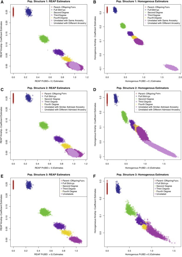
We compared REAP to relationship-estimation methods that assume population homogeneity under population-structure settings 1, 2, and 3. The pedigree relationships considered in our simulation study can be distinguished by their theoretical probability of zero-IBD sharing, and the theoretical kinship coefficients differentiate all of the relationship types except for the two types of first-degree relatives, parent-offspring relationships and full siblings. Figure 1 displays estimated kinship coefficients plotted against the estimated probability of zero-IBD sharing for the REAP estimators and the homogeneous-population relatedness estimators for the three population-structure settings. Figures 1B and 1D illustrate that relatedness-estimation methods that assume population homogeneity perform quite poorly for population-structure settings 1 and 2, both of which have assortative mating for ancestry: (1) Related individuals have a systematic inflation in the estimated degree of relatedness, (2) a large portion of unrelated pairs who have either the same ancestry or similar admixed ancestry have kinship-coefficient estimates that correspond to second- and third-degree relatives, and (3) unrelated individuals who have sufficiently different ancestry have estimated kinship-coefficient values that are systematically negative when the true kinship coefficient for these pairs is 0. Figure 1F, however, shows that for population-structure setting 3, in which there is no ancestry-related assortative mating, relatedness estimation methods that assume population homogeneity can give reliable relatedness inference for first-, second-, and many third-degree relatives.

Figure 1.

Kinship Coefficients Plotted against Zero-IBD-Sharing Probabilities

Estimated kinship coefficients plotted against zero-IBD-sharing-probability estimates for three population-structure settings.

(A, C, and E) Scatter plots comparing the REAP kinship-coefficient estimator from Equation 3 with the REAP zero-IBD-sharing-probability estimator from Equation 4 for population-structure settings 1 (A), 2 (C), and 3 (E).

(B, D, and F) Scatter plots comparing the homogeneous-population kinship-coefficient estimator from Equation 1 with the homogeneous-population zero-IBD-sharing-probability estimator from Equation 2 for population-structure settings 1 (B), 2 (D), and 3 (F). Zero-IBD-sharing-probability and kinship-coefficient estimates were calculated with 10,000 simulated random SNPs.

In contrast, Figures 1A, 1C, and 1E illustrate that REAP gives accurate kinship-coefficient and zero-IBD-sharing-probability estimates for all three population-structure settings. There is no overlap in the figures among the first-, second-, and third-degree relatives and no overlap between third-degree relatives and unrelated individuals in all three population-structure settings considered. Similar to what has been observed for relatedness estimators in homogeneous populations,¹² there is some overlap between third- and fourth-degree relatives and between fourth-degree relatives and unrelated individuals, although the degree of overlap is considerably less than that observed for methods assuming population homogeneity (e.g., Figure 1F). This is expected because the actual IBD sharing for pairs of relatives, except for parent-offspring relationships and monozygotic (MZ) twins, will vary around its expectation. REAP appropriately adjusts for ancestry in all population-structure settings, and there is no inflation of the relatedness estimates in the presence of population structure and assortative mating for ancestry. All unrelated individuals, even those who have substantially different admixture-ancestry distributions, have REAP kinship-coefficient estimates that are unbiased and close to the true kinship-coefficient value of 0. The REAP IBD-sharing-probability estimates are also robust in all population-structure settings considered, and Table 1 gives REAP IBD-sharing-probability averages and SDs for each relationship type for population-structure setting 2, in which there is both admixture and assortative mating for ancestry.

Table 1.

REAP IBD-Sharing-Probability Estimates for Population-Structure Setting 2

Outbred Relationship	δ0(Probability of IBD = 0)		δ1(Probability of IBD = 1)		δ2(Probability of IBD = 2)
	Theoretical Probability	REAP Estimate (SD)	Theoretical Probability	REAP Estimate (SD)	Theoretical Probability	REAP Estimate (SD)
Self	0	0 (0)	0	0.007 (0.013)	1	0.993 (0.013)
Parent-offspring pair	0	0 (0)	1	0.985 (0.020)	0	0.015 (0.020)
Full siblings	0.25	0.251 (0.019)	0.5	0.494 (0.038)	0.25	0.256 (0.028)
Second degree	0.5	0.501 (0.026)	0.5	0.485 (0.039)	0	0.014 (0.019)
Third degree	0.75	0.752 (0.030)	0.25	0.236 (0.043)	0	0.012 (0.017)
Fourth degree	0.875	0.873 (0.032)	0.125	0.116 (0.045)	0	0.011 (0.017)
Unrelated: similar ancestry	1	1.002 (0.032)	0	−0.003 (0.035)	0	0.001 (0.004)
Unrelated: different ancestry	1	0.980 (0.025)	0	0.019 (0.025)	0	0.001 (0.003)

In the table, δ₀, δ₁, and δ₂, are the probabilities that relationship types share 0, 1, and 2 alleles identical by descent, respectively. Results given in the table are the average REAP estimates for the IBD-sharing probabilities (and SDs) calculated with 10,000 simulated random SNPs for population-structure setting 2. The following abbreviations are used: IBD, identity by descent; REAP, relatedness estimation in admixed populations; and SD, standard deviation.

We also performed a simulation study by using estimated subpopulation allele frequencies for population-structure settings 1, 2, and 3. The frappe software program used for estimating the individual-ancestry proportions in the simulation studies also simultaneously estimates subpopulation allele frequencies at the SNPs, and Figure S2 displays estimated kinship coefficients plotted against the estimated probability of REAP zero-IBD sharing calculated with frappe-estimated SNP allele frequencies. There is little difference in relatedness inference with REAP when estimated versus true subpopulation allele frequencies are used for all population-structure settings considered.

Our simulation study illustrates that REAP performs well under various types of population-structure settings. REAP is robust to admixed ancestry from highly divergent populations, as well as to ancestry-related assortative mating.

Comparison of REAP and KING-Robust in Samples with Assortative Mating for Ancestry

The KING-robust method¹² was previously evaluated in structured samples that contain individuals from distinct subpopulations with no admixture. We evaluated KING-robust under population-structure setting 2, in which there is both ancestry admixture and ancestry-related assortative mating, and we compared the method to REAP. The KING-robust method calculates kinship coefficients, but not IBD-sharing probabilities, so we can only compare KING-robust to the REAP kinship-coefficient estimator and not to the REAP estimators for IBD-sharing probabilities. Table 2 gives the averages and SDs for the REAP and KING-robust kinship-coefficient estimators and for the homogeneous-population kinship-coefficient estimator from Equation 1 for population-structure setting 2. As previously discussed, the kinship-coefficient estimator that assumes population homogeneity gives biased kinship-coefficient estimates in this population-structure setting for all relationship types. KING-robust gives accurate kinship-coefficient estimates for all pairs of individuals who have similar admixed ancestry; however, for the unrelated pairs who have significantly different admixed-ancestry distributions, KING-robust gives systematically biased kinship-coefficient estimates. The true kinship coefficient for these pairs is 0, but the average KING-robust kinship-coefficient estimate is −0.135 with a SD of 0.040. REAP gives accurate kinship-coefficient estimates for all considered relationship types, including unrelated pairs who have significantly different admixed-ancestry distributions; the average REAP kinship-coefficient estimate for these pairs is −0.0001, and the SD is 0.005. Histograms for both the KING and REAP kinship-coefficient estimates for all unrelated pairs in the simulation study are given in Figure 2. The KING-robust histogram essentially shows two kinship-coefficient distributions; one distribution is centered close to 0 and corresponds to the unrelated pairs who have similar admixed ancestry, and the other distribution is centered around −0.14 and corresponds to the distribution of kinship-coefficient values for unrelated pairs who have different ancestry-admixture distributions. In contrast, all REAP kinship-coefficient values for the unrelated pairs are centered around the true kinship-coefficient value of 0.

Table 2.

Kinship-Coefficient Estimates for Population-Structure Setting 2 with REAP, KING-Robust, and the Homogeneous-Population Estimator

Outbred Relationship	ϕ (Kinship Coefficient)
	Theoretical Kinship Coefficient	REAP Estimate (SD)	Homogeneous Estimate (SD)	KING-Robust Estimate (SD)
Parent-offspring pair	0.25	0.251 (0.008)	0.291 (0.014)	0.249 (0.005)
Full siblings	0.25	0.251 (0.007)	0.291 (0.016)	0.251 (0.005)
Second degree	0.125	0.126 (0.006)	0.172 (0.016)	0.125 (0.007)
Third degree	0.0625	0.063 (0.005)	0.113 (0.016)	0.062 (0.008)
Fourth degree	0.03125	0.031 (0.005)	0.084 (0.014)	0.033 (0.008)
Unrelated: similar ancestry	0	−0.0001 (0.005)	0.054 (0.017)	−0.002 (0.010)
Unrelated: different ancestry	0	−0.0001 (0.005)	−0.055 (0.017)	−0.135 (0.040)

Kinship coefficients were estimated with the REAP kinship-coefficient estimator from Equation 3, the homogeneous-population kinship-coefficient estimator from Equation 1, and the KING-robust kinship-coefficient estimator. Results given in the table are the average of the kinship coefficients (and SDs) for each estimator calculated with 10,000 simulated random SNPs for population-structure setting 2. The following abbreviations are used: REAP, relatedness estimation in admixed populations; and SD, standard deviation.

Figure 2.

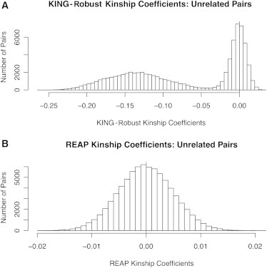
KING-Robust and REAP Kinship-Coefficient Histograms for Unrelated Pairs with Admixture

(A and B) Histograms of kinship coefficients estimated with the KING-robust kinship-coefficient estimator (A) and the REAP kinship-coefficient estimator from Equation 3 (B) for all pairs of unrelated individuals in population-structure setting 2. The vertical line at 0 in each histogram represents the true kinship coefficient for all pairs. Kinship-coefficient estimates were calculated with 10,000 simulated random SNPs.

Evaluation of REAP and KING-Robust When Related Individuals Have Different Ancestry

We also evaluated REAP and KING-robust under population structure 4, in which there are related individuals who have different admixed ancestry from two subpopulations as a result of disassortative mating. We define $D_{ij}=\left|a_i-a_j\right|$ as the absolute difference in the genome-wide ancestry proportions from subpopulation 1 for individuals i and j. For the relative pairs in population-structure setting 4, $D_{ij}$ ranges from 0 to 0.75. Table 3 gives averages and SDs for the REAP kinship-coefficient estimators for first-, second-, and third-degree relative pairs who have moderate to large ancestry differences under population structure 4, for which we define $0.125\le D_{ij}\le 0.375$ and $0.5\le D_{ij}\le 0.75$ to be “moderate” and “large” ancestry differences, respectively. REAP gives kinship-coefficient estimates that are consistent with first-degree relatives for parent-offspring pairs with moderate and large ancestry differences. Note that full siblings are not included in Table 3 because first-degree relative pairs of this type have similar genome-wide ancestry distributions. REAP also gives reliable relatedness estimates for second- and third-degree relatives with moderate and large ancestry differences. We also evaluated the performance of KING-robust when close relatives had large ancestry differences. The method gives reliable kinship-coefficient estimates for parent-offspring pairs with large ancestry differences; for these pairs, the average kinship coefficient is 0.223 (SD = 0.004). KING-robust, however, does not give accurate relatedness inference for second- and third-degree relatives with large ancestry differences. The kinship coefficient for second- and third-degree relatives is 0.125 and 0.0625, respectively, and the averages of the KING-robust kinship-coefficient estimates for these relative pairs are 0.021 (SD = 0.026) and 0.024 (SD = 0.014), respectively. In contrast, the REAP kinship-coefficient estimates for second- and third-degree relative pairs with large ancestry differences are 0.119 (SD = 0.006) and 0.059 (SD = 0.005), respectively. An advantage of REAP is that the method gives accurate relatedness inference for all pairs of individuals, even those who have substantially different ancestry-admixture distributions.

Table 3.

REAP Kinship-Coefficient Estimates for Relative Pairs with Moderate and Large Ancestry Differences for Population-Structure Setting 4

Outbred Relationship	Theoretical Kinship Coefficient	Moderate Ancestry Differencesa	Large Ancestry Differencesb
		REAP Estimate (SD)	REAP Estimate (SD)
Parent-offspring pair	0.25	0.233 (0.007)	0.232 (0.006)
Second degree	0.125	0.115 (0.006)	0.119 (0.006)
Third degree	0.0625	0.058 (0.005)	0.059 (0.005)

Kinship coefficients were estimated with the REAP kinship-coefficient estimator from Equation 3. Results given in the table are the average of the REAP kinship coefficients (and SDs) calculated with 10,000 simulated random SNPs for population-structure setting 4. The following abbreviations are used: REAP, relatedness estimation in admixed populations; and SD, standard deviation.

^aFor relative pairs with moderate ancestry differences, the absolute difference in genome-wide ancestry proportions from subpopulation 1 ranges from 0.125 to 0.375.

^bFor relative pairs with large ancestry differences, the absolute difference in genome-wide ancestry proportions from subpopulation 1 ranges from 0.5 to 0.75.

Assessment of REAP with Misspecification of the Ancestral Populations

We also investigated the impact on REAP when there is misspecification of the ancestral populations under population structure 3, in which individuals are admixed from three highly divergent populations. We considered two settings of misspecification. Misspecification setting 1 is similar to the previously discussed analysis for population-structure setting 3 when the ancestral populations are correctly specified except that (1) the number of ancestral populations is incorrectly set to K = 4 in the frappe software program for estimating the individual ancestry of the admixed individuals and that (2), in addition to the inclusion of the random samples of size 200 from each of the three subpopulations as fixed groups in the frappe analysis, a random sample of 200 individuals from a fourth subpopulation, from which the admixed individuals have no ancestry, is included as the fourth fixed group in the analysis. Misspecification setting 2 is also similar to the previously discussed analysis of population-structure setting 3 except that (1) the number of ancestral populations is incorrectly set to K = 2 in the frappe analysis and that (2) the random samples from two of the subpopulations are now combined and included as a single fixed group in the frappe analysis, and the random sample from the third subpopulation is included as the other fixed group. For each misspecification setting, individual-ancestry proportions and subpopulation allele frequencies were first estimated with the frappe software program, and the frappe estimates were then used for calculating the REAP kinship coefficients and IBD-sharing probabilities for all pairs of individuals. Figures S3 and S4 give the REAP kinship-coefficient estimates plotted against REAP zero-IBD-sharing-probability estimates for misspecification settings 1 and 2, respectively. Figure S3 illustrates that misspecification setting 1, for which the number of ancestral populations is misspecified to be four in the frappe analysis, has essentially no impact on relatedness inference with REAP. This can be seen in a comparison to Figure 1E, the corresponding REAP figure in which the ancestral populations are correctly specified. Figure S4 illustrates that REAP gives reliable relatedness inference for first-, second-, and third-degree relatives for misspecification setting 2, for which the number of ancestral populations is incorrectly specified to be two in the frappe analysis for population structure 3; however, the overlap of the fourth-degree relatives and unrelated pairs is considerably more than the overlap in Figure 1E as a result of the increase in the SDs of the REAP estimates when the number of ancestral populations is misspecified to be two. Table S1 gives the averages and SDs of the REAP kinship coefficients for misspecification setting 2, as well as the setting when the ancestral populations are correctly specified. The SDs of the REAP estimates for all relationship types are larger for misspecification setting 2 than are the SDs of the REAP estimates when the ancestral populations are correctly specified.

Resolution of Relationship Inference with REAP for Different SNP Densities

For population-structure setting 2, we also performed simulation studies by using 5K random SNPs (where K = 1,000) to see how the resolution of REAP for identifying and distinguishing relative pairs is impacted when the number of SNPs is reduced by 50%. Figure S5 gives the REAP kinship-coefficient estimates plotted against REAP zero-IBD-sharing-probability estimates when 5K SNPs were used. Figure 1C gives the corresponding REAP plot for population structure 2 when 10K SNPs were used. For both the 5K and 10K SNP analyses, the REAP-estimated kinship coefficients and zero-IBD-sharing probabilities are centered around their respective expected values for all relationship types. In the figures, there is no overlap among the first-, second-, and third-degree relatives or among the third-degree relatives and unrelated individuals. However, when 5K SNPs were used, there was substantially more overlap between third- and fourth-degree relatives and between fourth-degree relatives and unrelated individuals than when 10K SNP were used as a result of the higher SD of the REAP estimators when the number of random SNPs used for estimating relatedness was reduced by 50%. For the 5K SNP analysis, the REAP kinship-coefficient averages for parent-offspring pairs, full siblings, and second-degree, third-degree, and fourth-degree relative pairs are 0.252 (SD = 0.011), 0.252 (SD = 0.009), 0.126 (SD = 0.009), 0.062 (SD = 0.008), and 0.031 (SD = 0.008), respectively. When 5K SNPs were used, the REAP-estimated kinship-coefficient averages for unrelated pairs who have both similar and different admixed-ancestry distributions are −0.00007 (SD = 0.007) and −0.00006 (SD = 0.007), respectively. The averages and SDs of the REAP kinship-coefficient estimates when 10K SNPs were used for all relationship types are given in Table 2.

Estimating Inbreeding Coefficients in Structured Populations

We estimated inbreeding coefficients for population-structure settings 1, 2, and 3 by using the REAP inbreeding-coefficient estimator ${\hat{h}}_i^A$ (Equation 5) and the inbreeding-coefficient estimator ${\hat{h}}_i$ (Equation 6) for homogeneous populations. All individuals in the simulation study are outbred, so the true inbreeding coefficient is 0 for every individual. Table 4 reports the averages of the inbreeding-coefficient values (and SDs) for the two estimators for each of the population-structure settings. For population-structure settings 1 and 2, the inbreeding-coefficient estimates are highly inflated with the use of ${\hat{h}}_i$, the estimator that assumes population homogeneity; the averages of the inbreeding coefficients for this estimator are 0.094 and 0.056 for population-structure settings 1 and 2, respectively. In contrast, the REAP inbreeding-coefficient estimator ${\hat{h}}_i^A$ has an average of −0.002 and −0.007 for population-structure settings 1 and 2, respectively. For population-structure setting 3, in which there is no assortative mating for ancestry, both of the inbreeding-coefficient estimators give average inbreeding estimates that are close to 0; the average values for ${\hat{h}}_i^A$ and ${\hat{h}}_i$ are −0.007 and 0.010, respectively.

Table 4.

Inbreeding-Coefficient Estimates with REAP and the Homogeneous-Population Estimator

Population Structure	Inbreeding Coefficient
	True Inbreeding Coefficient	REAP Estimate (SD)	Homogeneous Estimate (SD)
1	0	−0.002 (0.018)	0.094 (0.017)
2	0	0.007 (0.016)	0.056 (0.023)
3	0	−0.007 (0.019)	0.010 (0.031)

Inbreeding coefficients were estimated with the REAP inbreeding-coefficient estimator from Equation 5 and the homogeneous-population inbreeding-coefficient estimator from Equation 6 for population-structure settings 1, 2, and 3. Results given in the table are the average of the inbreeding-coefficient estimates (and SDs) for each estimator calculated with 10,000 simulated random SNPs. The following abbreviations are used: REAP, relatedness estimation in admixed populations; and SD, standard deviation.

HapMap MXL Data

The HapMap MXL samples have well-documented parent-offspring relationships.¹⁵ A recent relationship-inference analysis of these samples identified additional first- and second-degree relationships that were previously unreported.²⁴ We estimate IBD-sharing probabilities and kinship coefficients in this sample by using REAP to verify previously identified relatives and to identify third- and fourth-degree relationships that had not been reported. We first used the frappe software program to estimate the genome-wide proportions of European, African, and Native American ancestry for the 86 sample individuals who have available genotype data in HapMap MXL. We set the number of ancestral populations at K = 3 in the frappe analysis, for which the HapMap CEU (Utah residents with ancestry from northern and western Europe from the Centre d'Étude du Polymorphisme Humain collection) and YRI (Yoruba in Ibadan, Nigeria) samples were used for European and African ancestry, respectively, and for which the Human Genome Diversity Project²⁵ (HGDP) samples from the Americas were used for Native American ancestry. The surrogate HGDP sample for Native American ancestry includes 8 Surui, 22 Maya, 13 Karitiana, 14 Pima, and 6 Colombian individuals. In the frappe analysis, 150,872 autosomal SNPs that were genotyped in both the HapMap and HGDP datasets were used. Figure 3 presents a bar plot of the results from the frappe analysis of the HapMap MXL samples; the HGDP Native American and HapMap CEU and YRI samples were included in the analysis as fixed groups, and proportional ancestry was estimated for the 86 HapMap MXL genotyped individuals. In the bar plot of frappe ancestry estimates, individuals (vertical bars) are arranged in increasing order (left to right) of genome-wide European ancestry proportion. All HapMap MXL individuals have modest African ancestry (5% on average [SD = 0.02]); most of their ancestry is European and Native American at around 50% and 45%, respectively, on average. The proportion of European and Native American ancestry is quite variable; the Native American ancestry proportion ranges from 0.04 to 0.81 and has a SD of 0.15, and the European ancestry proportion ranges from 0.18 to 0.93 and also has a SD of 0.15.

Figure 3.

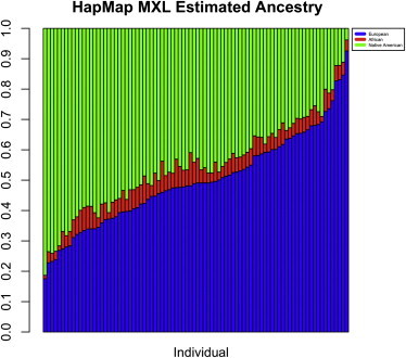
Individual-Ancestry Estimates for HapMap MXL

Individual-ancestry estimates for 86 HapMap MXL sample individuals from a supervised structure analysis with the frappe software program. In the figure, each individual is represented by a vertical bar; European (HapMap CEU) and African (HapMap YRI) ancestry contributions are in blue and red, respectively, and Native American (HGDP samples from the Americas) ancestry contributions are in green.

We calculated REAP kinship-coefficient and IBD-sharing-probability estimates for all pairs of individuals in HapMap MXL by using the frappe-estimated individual-ancestry vectors $\hat{\mathbf{a}}$ and the estimated subpopulation allele frequencies ${\hat{\mathbf{q}}}^{\mathbf{s}}$ for each SNP s. Figure 4 displays REAP-estimated kinship coefficients plotted against REAP zero-IBD-sharing-probability estimates for all pairs of individuals in the HapMap MXL sample. We used previously proposed inference criteria¹² based on estimates of zero-IBD-sharing probability and kinship coefficients for relationship classification. The inference criteria, derived with powers of two, is the natural scale of the kinship coefficients and zero-IBD-sharing probabilities in noninbred populations, and in our simulation studies, the relationship-classification criteria performed well for all relationship types. REAP identifies all of the documented parent-offspring relationships as well as verifies the additional first- and second-degree relatives who were previously identified.²⁴ REAP also identifies additional third- and fourth-degree relationships that have not previously been reported. All relative pairs in the HapMap MXL sample identified by REAP are given in Table S2.

Figure 4.

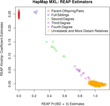
REAP Kinship Coefficients versus Zero-IBD-Sharing Probabilities for HapMap MXL

REAP kinship-coefficient estimates are plotted against REAP zero-IBD-sharing-probability estimates for the HapMap MXL sample. REAP estimates were calculated with the kinship-coefficient and zero-IBD-sharing-probability estimators from Equations 3 and 4, respectively. Relative pairs were classified on the basis of kinship-coefficient and zero-IBD-sharing-probability estimates.

Figure 5 is a REAP-reconstructed large extended pedigree connecting four HapMap MXL families: M008, 2382, M011, and M012. We can also reconstruct this extended pedigree by connecting the four families by using the previously identified²⁴ first- and second-degree relatives. All third- and fourth-degree relationships indicated by the extended pedigree have REAP-estimated kinship coefficients and IBD-sharing probabilities that are consistent for relative pairs. Consider, for example, individual NA19665, who is the offspring in trio M012. This individual has a third-degree relationship with full siblings NA19660 and NA19672 in the reconstructed pedigree. For NA19665, the REAP kinship-coefficient estimates for the relationships with siblings NA19660 and NA19672 are 0.04 and 0.05, respectively, and the REAP zero-IBD-sharing-probability estimates are 0.85 and 0.80, respectively. NA19665 is also a fourth-degree relative of both NA19662 and NA19685 in the reconstructed pedigree; the REAP zero-IBD-sharing-probability estimates for the relationships with NA19662 and NA19685 are 0.93 and 0.92, respectively, and the corresponding REAP kinship-coefficient estimates are both equal to 0.02. Interestingly, one pair of individuals in this figure, NA19665 and NA19660, has a third-degree relationship from the reconstructed pedigree, but the pair would be classified as fourth-degree relatives on the basis of the inference criteria that we used. As previously mentioned, some overlap between third- and fourth-degree relatives is expected because the proportion of the genome that is shared identically by descent for relatives will vary around its expected value as a result of the stochastic nature of segregation and recombination.²⁶

Figure 5.

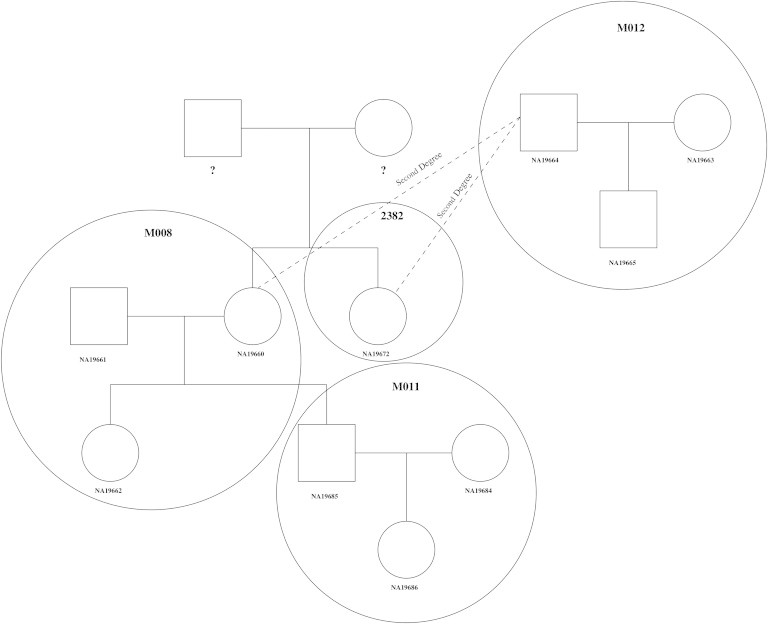
Example of an Extended Pedigree Reconstructed with REAP in HapMap MXL

REAP-inferred pedigree relationships for four HapMap-reported pedigrees from the MXL sample are given. HapMap-reported pedigree relationships are circled, and HapMap-reported pedigree identification numbers (M008, 2382, M011, and M012) are given in bold font in each of the circles.

Figure 6 displays pedigree relationships that connect the HapMap MXL families M007 and M032, in which individual NA19657, who is the mother in trio M007, is estimated to have a third-degree relationship with the father (NA19786) of trio M032 and a fourth-degree relationship with the mother (NA19785) of trio M032. The REAP estimates of kinship coefficients and zero-IBD-sharing probabilities for individuals NA19657 and NA19786 are 0.06 and 0.73, respectively; the REAP estimates of kinship coefficients and zero-IBD-sharing probabilities for individuals NA19657 and NA19785 are 0.02 and 0.91, respectively. NA19657 has a complex relationship with NA19787, the offspring in family M032, because the two are related through NA19787's maternal and paternal lineage. The REAP-estimated kinship coefficient for NA19657 and NA19787 is 0.05, and the REAP zero-IBD-sharing-probability estimate is 0.76. Based on the reconstructed pedigree, the theoretical kinship coefficient and zero-IBD-sharing probability for the pair are 0.046875 and 0.8203125, respectively. The two parents (NA19785 and NA19786) of NA19787 in trio M032 are inferred to be unrelated because their REAP kinship-coefficient and zero-IBD-sharing-probability estimates are 0.009 and 0.99, respectively.

Figure 6.

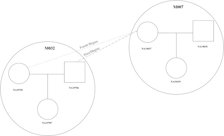
Example of Two HapMap MXL Pedigrees Connected with REAP

Pedigree relationships for two HapMap-reported pedigrees from the MXL sample are given. HapMap-reported pedigree relationships are circled, and HapMap-reported pedigree identification numbers (M007 and M032) are given in bold font in each of the circles.

Figure S6 displays a histogram of REAP-estimated kinship-coefficient values for 3,666 pairs of individuals who have kinship-coefficient estimates that are less than 0.045, which is around the lower level of kinship-coefficient values that would be expected for most third-degree relatives. The kinship coefficients are approximately normally distributed with a mean of −0.0002 and a SD of 0.003, and the values range from −0.010 to 0.039. Because the mean kinship coefficient for unrelated individuals should be close to 0, the lower bound of this range can roughly be regarded as the maximum deviation of an estimate from the mean. We estimated the two-tailed 95% confidence interval (adjusted for multiple tests by Bonferroni correction) to be (−0.014, 0.014) by using all REAP kinship coefficients that are less than 0.045. Therefore, the right tail of the kinship-coefficient distribution for unrelated individuals should not go beyond around 0.014, and kinship coefficients that are greater than this should correspond to relative pairs. All third- and fourth-degree relatives given in the constructed pedigrees of Figures 5 and 6 have kinship coefficients that are greater than the estimated kinship-coefficient upper bound for unrelated pairs.

WHI-SHARe Data

The WHI is a long-term national health study focused on identifying risk factors for common diseases in postmenopausal women. A total of 161,838 women aged 50–79 years old were recruited from 40 clinical centers in the United States between 1993 and 1998. The WHI consists of an observational study, two clinical trials of postmenopausal hormone therapy (estrogen alone and estrogen plus progestin), a calcium and vitamin D supplement trial, and a dietary modification trial.²⁷ The WHI-SHARe minority cohort of women from the WHI consists of 8,421 self-reported African Americans and 3,587 self-reported Hispanics who provided consent for DNA analysis. All samples were genotyped at Affymetrix on the Genome-wide Human SNP Array 6.0. There is no available pedigree or genealogical information for the WHI-SHARe sample, so we used REAP to identify related individuals in this admixed sample.

We used the frappe software to estimate individual ancestry for every individual in the WHI-SHARe sample. As in our REAP analysis of the HapMap MXL sample (discussed in the previous subsection), the HapMap CEU, HapMap YRI, and HGDP samples from the Americas were used as surrogates for European ancestry, African ancestry, and Native American ancestry, respectively. Because there are some WHI-SHARe individuals who self-reported that they had East Asian ancestry, we also included HGDP East Asian samples in the frappe analysis. We used 656,852 autosomal SNPs genotyped in the WHI-SHARe sample and set the number of ancestral populations at K = 4 in the frappe analysis, in which the HapMap CEU and YRI samples, HGDP samples from the Americas, and East Asian samples were included as fixed groups. Proportional ancestry was estimated for all 12,008 individuals. In the frappe analysis, we included SNPs genotyped in WHI-SHARe, but not in both the HapMap and HGDP samples; this differs from the frappe analysis discussed in the previous subsection. An advantage of frappe is that the software allows SNPs that might not be genotyped on all platforms to contribute to individual ancestry while simultaneously estimating the ancestral allele frequencies for these SNPs. We also performed the frappe analysis for the WHI-SHARe sample by using only overlapping SNPs in all three study samples, and we found that there was little difference in the individual-ancestry estimates. For the self-reported African Americans, the average frappe-estimated European, African, Native American, and East Asian ancestry proportions are 0.21 (SD = 0.15), 0.76 (SD = 0.15), 0.02 (SD = 0.02), and 0.01 (SD = 0.02), respectively. For the self-reported Hispanics, the average estimated European, African, Native American, and East Asian ancestry proportions are 0.60 (SD = 0.20), 0.06 (SD = 0.12), 0.32 (SD = 0.20), and 0.02 (SD = 0.04), respectively. The ancestry-admixture distribution is quite different for the African Americans and the Hispanics, as expected, but there is also large variation in continental admixture within each group.

We estimated IBD-sharing probabilities and kinship coefficients for all possible pairs in the WHI-SHARe sample (72,090,028 pairs) by using REAP with the frappe-estimated genome-wide ancestry proportions for each individual and with the frappe-estimated ancestral allele frequencies for the SNPs. Figure 7 displays REAP-estimated kinship coefficients plotted against REAP zero-IBD-sharing-probability estimates. MZ twins, parent-offspring pairs, full siblings, second-degree relatives, and third-degree relatives were identified in both the self-reported African American and Hispanic samples, for which we used the same relationship-classification criteria¹² previously discussed. A total of 363 and 156 close relative pairs (up to the third degree) were identified in the African American and Hispanic samples, respectively. Table 5 gives the number of pairs identified for each relationship type within each race or ethnic group.

Figure 7.

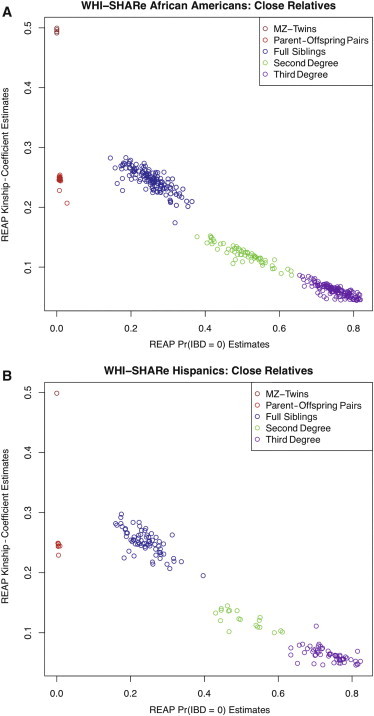
REAP Kinship Coefficients versus Zero-IBD-Sharing Probabilities for WHI-SHARe

(A and B) REAP kinship-coefficient estimates are plotted against REAP zero-IBD-sharing-probability estimates for the WHI-SHARe self-reported African Americans and self-reported Hispanics, respectively. REAP estimates were calculated with the kinship-coefficient and zero-IBD-sharing-probability estimators from Equations 3 and 4, respectively.

Table 5.

Close Relative Pairs Inferred by REAP for WHI-SHARe

Outbred Relationship	Self-Reported African American Relatives	Self-Reported Hispanic Relatives
MZ twins	4	1
Parent-offspring pair	20	8
Full siblings	139	71
Second degree	60	19
Third degree	140	57

For each relationship type, the total number of relative pairs identified by REAP in the self-reported African Americans and self-reported Hispanics in WHI-SHARe is given. The following abbreviations are used: REAP, relatedness estimation in admixed populations; WHI-SHARe, Women's Health Initiative SNP Health Association Resource; and MZ, monozygotic.

Figures S7 and S8 give histograms of all pairwise REAP-estimated kinship coefficients that are less than 0.045 for the self-reported WHI-SHARe African Americans and Hispanics, respectively. The kinship coefficients are approximately normally distributed for both groups. The African Americans have a mean kinship coefficient of −0.00005 and a SD of 0.002, whereas Hispanics have a mean kinship coefficient of 0.00002 and a SD of 0.003. Using all REAP kinship coefficients less than .045, we estimated the two-tailed 95% confidence intervals (adjusted for multiple tests by Bonferroni correction) for the African Americans and the Hispanics to be (−0.014, 0.014) and (−0.015, 0.015), respectively. So, similar to the upper bound that we estimated for REAP kinship coefficients of unrelated individuals in the HapMap MXL sample, we would not expect unrelated pairs to have REAP kinship-coefficient estimates greater than around 0.015 in WHI-SHARe.

Interestingly, we identified individuals who are second- and third-degree relative pairs as determined by REAP but who have a different self-reported race or ethnicity, e.g., one individual is a self-reported African American and the other is a self-reported Hispanic. Table 6 gives 11 REAP-inferred relative pairs discordant for self-reported race or ethnicity and gives their frappe-estimated genome-wide European, African, Native American, and East Asian ancestry proportions. Notice that all of the identified relative pairs, except for discordant pair 6, have substantially different ancestry distributions. Some of the relative pairs combine to form larger groups of relatives in WHI-SHARe. These relatives would not have been identified had we restricted our relatedness analysis to only those individuals who self-reported the same race or ethnic group. An advantage of the REAP approach is that robust relatedness estimates can be obtained for all individuals, even for individuals who have different admixed-ancestry distributions and self-identify in different population subgroups.

Table 6.

REAP-Inferred Close Relative Pairs with Different Self-Reported Race or Ethnicity in WHI-SHARe

Discordant Pair	Self-Reported Race or Ethnicity	Individual Ancestry Proportionsa				REAP Kinship Coefficient	REAP IBD = 0 Probability	Inferred Relationship
		European	African	Native American	East Asian
1	Hispanic	0.43	0.49	0.00	0.08	0.06	0.80	third degree
	African American	0.23	0.75	0.02	0.00
2	Hispanic	0.45	0.33	0.22	0.00	0.11	0.57	second degree
	African American	0.48	0.49	0.03	0.00
3	Hispanic	0.41	0.06	0.22	0.31	0.05	0.82	third degree
	African American	0.18	0.69	0.00	0.13
4	Hispanic	0.41	0.06	0.22	0.31	0.06	0.82	third degree
	African American	0.06	0.78	0.00	0.16
5	Hispanic	0.41	0.06	0.22	0.31	0.07	0.79	third degree
	African American	0.17	0.64	0.00	0.19
6	Hispanic	0.42	0.57	0.01	0.00	0.07	0.77	third degree
	African American	0.48	0.50	0.02	0.00
7	Hispanic	0.33	0.10	0.18	0.39	0.05	0.80	third degree
	African American	0.83	0.00	0.00	0.17
8	Hispanic	0.55	0.05	0.05	0.35	0.05	0.82	third degree
	African American	0.83	0.00	0.00	0.17
9	Hispanic	0.57	0.04	0.13	0.26	0.06	0.81	third degree
	African American	0.35	0.43	0.00	0.22
10	Hispanic	0.79	0.02	0.00	0.18	0.05	0.81	third degree
	African American	0.35	0.43	0.00	0.22
11	Hispanic	0.41	0.02	0.34	0.24	0.05	0.80	third degree
	African American	0.19	0.63	0.00	0.17

^aIndividual-ancestry estimates are from a supervised structure analysis with the frappe software program. The following abbreviations are used: WHI-SHARe, Women's Health Initiative SNP Health Association Resource; REAP, relatedness estimation in admixed populations; and IBD, identity be descent.

We also used the software package PLINK⁴ to estimate all pairwise relationships in WHI-SHARe. PLINK uses a MOM approach that assumes random mating and population homogeneity for estimating relatedness. There are 8,932 pairs of individuals who have estimated kinship coefficients greater than 0.088 with PLINK, for which 0.088 is a lower-limit kinship-coefficient threshold that has been proposed for second-degree relatives.¹² In contrast, according to the REAP kinship-coefficient estimator, there are 344 pairs of WHI-SHARe individuals who have an estimated kinship coefficient greater than 0.088. With the MOM kinship-estimation method implemented in PLINK, there are thousands of unrelated pairs and distantly related pairs who have estimated kinship coefficients that correspond to what would be expected for close relatives, illustrating the large bias that can be introduced with the use of relatedness-estimation methods that assume random mating and population homogeneity in samples with population stratification and ancestry admixture.

Assessment of Computation Time

We evaluated the computation time of the REAP software for two datasets by using a single machine with Intel Xeon quad-core 2.66 GHz processors with 16 GB of random-access memory. The REAP software calculates kinship coefficients and zero-IBD-sharing-probability estimates for all pairs of individuals in a sample, as well as inbreeding coefficients for the sample individuals. For a sample with 2,560 individuals and 100,000 SNPs, the REAP analysis took approximately 1 hr and 31 min. The REAP analysis of the HapMap MXL sample with 86 individuals and 150,872 SNPs took approximately 20 s. The large difference in computation time is due to the fact that the first sample had 2,560 individuals and 3,275,520 pairs, whereas the second sample had 86 individuals and only 3,655 pairs. For a given dataset, the computation time scales linearly with the number of SNPs and quadratically with the number of individuals.

Discussion

Given the advancements in high-density genome scans, it is now common for GWASs to have data for thousands of individuals. The observations in these studies can have several sources of dependence (including population structure and relatedness among the sample individuals), some of which might be known and others of which might be unknown. It is well known that inclusion of related individuals in association studies without proper adjustment for the correlated genotypes among relatives can lead to spurious associations. Statistical methods used for identifying related individuals from large-scale genetic data often make simplifying assumptions, such as random mating and population homogeneity, which are not valid for many populations. We specifically address the problem of relatedness estimation in structured populations with admixed ancestry. We developed a method, REAP, for robust estimation of IBD-sharing probabilities and kinship coefficients in samples from admixed populations.

In simulation studies containing both related and unrelated individuals with various types of population-structure settings, including ancestry admixture and ancestry-related mating, we demonstrated that REAP provides accurate IBD-sharing probabilities and kinship-coefficient estimates for relative pairs up to degree four. We also showed in simulation studies that admixture alone does not significantly distort the kinship-coefficient and IBD-sharing-probability estimates for the relatedness-estimation methods that assume population homogeneity. However, we did demonstrate that admixture with ancestry-related assortative mating leads to inflated relatedness estimates if not properly taken into account. A strong assumption of random mating that is independent of ancestry, however, is often untenable because human populations do not mate at random, and there is also evidence of ancestry-related assortative mating within ethnic groups.^13,14 One advantage of REAP is that the method is robust to any pattern of assortative mating for ancestry.

We applied REAP to the MXL HapMap population sample and confirmed previously identified first- and second-degree relatives. REAP also identified third- and fourth-degree relatives who have not previously been reported. We also applied REAP to the WHI-SHARe African American and Hispanic samples, in which we identified 530 first-, second-, and third-degree relative pairs. In contrast, when we used the MOM relatedness estimators implemented in the PLINK software package (these estimators assume random mating and population homogeneity), more than 8,900 pairs had kinship coefficients corresponding to first- and second-degree relatives; according to our analysis with REAP, the vast majority of these pairs are unrelated and have REAP kinship-coefficient estimates close to 0 after adjustment for the genome-wide admixed-ancestry distributions of the sample individuals.

It is possible for close relatives to have substantially different ancestry distributions. For example, when two individuals from different populations mate, they produce admixed offspring who will have different ancestry distributions from both parents. In simulation studies, we investigated the impact of ancestry differences among both related and unrelated individuals by using REAP and the recently proposed KING-robust kinship-coefficient estimator. We demonstrated that REAP gives reliable relatedness estimates for all pairs of individuals, even for relative pairs who have significantly different ancestry distributions. In contrast, the KING-robust method can give incorrect relatedness inference for close relative pairs with different admixed ancestry, and unrelated pairs with different ancestry have kinship-coefficient estimates that are systematically negative. The robustness of REAP allows for the identification of relatives who have very different admixed-ancestry distributions and self-identify in different ethnic or nationality groups. When we applied REAP to the WHI-SHARe sample, 11 second- and third-degree relative pairs with different self-reported races or ethnicities were identified; ten of these pairs had frappe-estimated genome-wide ancestry distributions that were significantly different.

For samples with admixed ancestry, statistical methods^22,28,29 have been proposed for estimating ancestry at specific genomic locations with the use of high-density genotype data. Local-ancestry estimates are commonly used for complex-trait admixture mapping, for which loci that have unusual deviations of local ancestry and that are significantly associated with a trait are identified. REAP can also incorporate local-ancestry estimates for relatedness inference in admixed populations. We found little difference in the REAP estimates when we used local versus genome-wide ancestry in our simulation studies of relatedness and ancestry admixture.

We estimated REAP kinship coefficients and IBD-sharing probabilities by conditioning on individual ancestry and subpopulation allele frequencies. Software programs are available for simultaneously estimating ancestry admixture proportions in samples from admixed populations, as well as allele frequencies of the subpopulations. When the number of ancestral populations is unknown or when surrogates for an ancestral population are not adequately represented in the ancestry analysis, there can be a bias in the individual-ancestry estimates and in the allele-frequency estimates; as a result, there will be a bias in the REAP relatedness estimates. The REAP inbreeding-coefficient estimator can be used as a simple diagnostic tool for identifying individual-ancestry misspecification and for detecting bias in estimates of subpopulation allele frequencies. The expected inbreeding coefficient is 0 for admixed individuals who are not inbred, and the REAP inbreeding-coefficient estimates will be inflated for individuals who have estimated individual ancestry that does not correspond to their true ancestry or when the there is a bias in the subpopulation allele frequencies.

Estimating heritability in admixed populations is a research area of current interest. Recently, methods for estimating the proportion of variation explained by GWAS SNPs for complex traits have been proposed^30,31 for homogeneous-population samples, for which the heritability estimates rely on accurate kinship estimation for all pairs of individuals. The relatedness-estimation methods that have previously been used for obtaining SNP-based heritability estimates, however, are only valid for unstructured populations, and in the presence of population stratification, heritability estimates from GWAS data can be highly inflated.³² Using REAP-estimated kinship coefficients and IBD-sharing probabilities could be one approach to obtaining valid SNP-based heritability estimates in GWAS samples with population stratification because robust IBD-sharing probabilities and kinship-coefficient estimates can be obtained with REAP in this setting.

We have implemented the REAP IBD-sharing probabilities and kinship-coefficient estimators in the REAP software package. The source code will be freely downloadable (see Web Resources).

Web Resources

The URL for data presented herein is as follows:

• REAP source code, http://faculty.washington.edu/tathornt/software/index.html

References

- 1.Slager S.L., Schaid D.J. Evaluation of candidate genes in case-control studies: A statistical method to account for related subjects. Am. J. Hum. Genet. 2001;68:1457–1462. doi: 10.1086/320608. [DOI] [PMC free article] [PubMed] [Google Scholar]
- 2.Bourgain C., Hoffjan S., Nicolae R., Newman D., Steiner L., Walker K., Reynolds R., Ober C., McPeek M.S. Novel case-control test in a founder population identifies P-selectin as an atopy-susceptibility locus. Am. J. Hum. Genet. 2003;73:612–626. doi: 10.1086/378208. [DOI] [PMC free article] [PubMed] [Google Scholar]
- 3.Thornton T., McPeek M.S. Case-control association testing with related individuals: a more powerful quasi-likelihood score test. Am. J. Hum. Genet. 2007;81:321–337. doi: 10.1086/519497. [DOI] [PMC free article] [PubMed] [Google Scholar]
- 4.Purcell S., Neale B., Todd-Brown K., Thomas L., Ferreira M.A.R., Bender D., Maller J., Sklar P., de Bakker P.I., Daly M.J. PLINK: A tool set for whole-genome association and population-based linkage analyses. Am. J. Hum. Genet. 2007;81:559–575. doi: 10.1086/519795. [DOI] [PMC free article] [PubMed] [Google Scholar]
- 5.Choi Y., Wijsman E.M., Weir B.S. Case-control association testing in the presence of unknown relationships. Genet. Epidemiol. 2009;33:668–678. doi: 10.1002/gepi.20418. [DOI] [PMC free article] [PubMed] [Google Scholar]
- 6.Day-Williams A.G., Blangero J., Dyer T.D., Lange K., Sobel E.M. Linkage analysis without defined pedigrees. Genet. Epidemiol. 2011;35:360–370. doi: 10.1002/gepi.20584. [DOI] [PMC free article] [PubMed] [Google Scholar]
- 7.Devlin B., Roeder K. Genomic control for association studies. Biometrics. 1999;55:997–1004. doi: 10.1111/j.0006-341x.1999.00997.x. [DOI] [PubMed] [Google Scholar]
- 8.Pritchard J.K., Stephens M., Donnelly P. Inference of population structure using multilocus genotype data. Genetics. 2000;155:945–959. doi: 10.1093/genetics/155.2.945. [DOI] [PMC free article] [PubMed] [Google Scholar]
- 9.Price A.L., Patterson N.J., Plenge R.M., Weinblatt M.E., Shadick N.A., Reich D. Principal components analysis corrects for stratification in genome-wide association studies. Nat. Genet. 2006;38:904–909. doi: 10.1038/ng1847. [DOI] [PubMed] [Google Scholar]
- 10.Thornton T., McPeek M.S. ROADTRIPS: Case-control association testing with partially or completely unknown population and pedigree structure. Am. J. Hum. Genet. 2010;86:172–184. doi: 10.1016/j.ajhg.2010.01.001. [DOI] [PMC free article] [PubMed] [Google Scholar]
- 11.Kang H.M., Sul J.H., Service S.K., Zaitlen N.A., Kong S.Y., Freimer N.B., Sabatti C., Eskin E. Variance component model to account for sample structure in genome-wide association studies. Nat. Genet. 2010;42:348–354. doi: 10.1038/ng.548. [DOI] [PMC free article] [PubMed] [Google Scholar]
- 12.Manichaikul A., Mychaleckyj J.C., Rich S.S., Daly K., Sale M., Chen W.M. Robust relationship inference in genome-wide association studies. Bioinformatics. 2010;26:2867–2873. doi: 10.1093/bioinformatics/btq559. [DOI] [PMC free article] [PubMed] [Google Scholar]
- 13.Sebro R., Hoffman T.J., Lange C., Rogus J.J., Risch N.J. Testing for non-random mating: Evidence for ancestry-related assortative mating in the Framingham heart study. Genet. Epidemiol. 2010;34:674–679. doi: 10.1002/gepi.20528. [DOI] [PMC free article] [PubMed] [Google Scholar]
- 14.Risch N., Choudhry S., Via M., Basu A., Sebro R., Eng C., Beckman K., Thyne S., Chapela R., Rodriguez-Santana J.R. Ancestry-related assortative mating in Latino populations. Genome Biol. 2009;10:R132. doi: 10.1186/gb-2009-10-11-r132. [DOI] [PMC free article] [PubMed] [Google Scholar]
- 15.International HapMap 3 Consortium Integrating common and rare genetic variation in diverse human populations. Nature. 2010;467:52–58. doi: 10.1038/nature09298. [DOI] [PMC free article] [PubMed] [Google Scholar]
- 16.Abney M. A graphical algorithm for fast computation of identity coefficients and generalized kinship coefficients. Bioinformatics. 2009;25:1561–1563. doi: 10.1093/bioinformatics/btp185. [DOI] [PMC free article] [PubMed] [Google Scholar]
- 17.Zheng, Q., and Bourgain, C. (2009). KinInbcoef: Calculation of kinship and inbreeding coefficients (http://galton.uchicago.edu/∼mcpeek/software/index.html).
- 18.S.A.G.E. (2009). Statistical Analysis for Genetic Epidemiology, Release 6.0.1 (http://darwin.cwru.edu/).
- 19.Balding D.J., Nichols R.A. A method for quantifying differentiation between populations at multi-allelic loci and its implications for investigating identity and paternity. Genetica. 1995;96:3–12. doi: 10.1007/BF01441146. [DOI] [PubMed] [Google Scholar]
- 20.Lawrance A.J. On Conditional and Partial Correlation. Am. Stat. 1976;30:146–149. [Google Scholar]
- 21.Tang H., Peng J., Wang P., Risch N.J. Estimation of individual admixture: Analytical and study design considerations. Genet. Epidemiol. 2005;28:289–301. doi: 10.1002/gepi.20064. [DOI] [PubMed] [Google Scholar]
- 22.Tang H., Coram M., Wang P., Zhu X., Risch N. Reconstructing genetic ancestry blocks in admixed individuals. Am. J. Hum. Genet. 2006;79:1–12. doi: 10.1086/504302. [DOI] [PMC free article] [PubMed] [Google Scholar]
- 23.Wright S. The genetical structure of populations. Ann. Eugen. 1951;15:323–354. doi: 10.1111/j.1469-1809.1949.tb02451.x. [DOI] [PubMed] [Google Scholar]
- 24.Pemberton T.J., Wang C., Li J.Z., Rosenberg N.A. Inference of unexpected genetic relatedness among individuals in HapMap Phase III. Am. J. Hum. Genet. 2010;87:457–464. doi: 10.1016/j.ajhg.2010.08.014. [DOI] [PMC free article] [PubMed] [Google Scholar]
- 25.Li J.Z., Absher D.M., Tang H., Southwick A.M., Casto A.M., Ramachandran S., Cann H.M., Barsh G.S., Feldman M., Cavalli-Sforza L.L., Myers R.M. Worldwide human relationships inferred from genome-wide patterns of variation. Science. 2008;319:1100–1104. doi: 10.1126/science.1153717. [DOI] [PubMed] [Google Scholar]
- 26.Visscher P.M., Hill W.G., Wray N.R. Heritability in the genomics era—concepts and misconceptions. Nat. Rev. Genet. 2008;9:255–266. doi: 10.1038/nrg2322. [DOI] [PubMed] [Google Scholar]
- 27.Prentice R.L., Anderson G., Cummings S., Freedman L.S., Furberg C., Henderson M., Johnson S.R., Kuller L., Manson J., Oberman A. Design of the Women's Health Initiative clinical trial and observational study. Control. Clin. Trials. 1998;19:61–109. doi: 10.1016/s0197-2456(97)00078-0. [DOI] [PubMed] [Google Scholar]
- 28.Sankararaman S., Sridhar S., Kimmel G., Halperin E. Estimating local ancestry in admixed populations. Am. J. Hum. Genet. 2008;82:290–303. doi: 10.1016/j.ajhg.2007.09.022. [DOI] [PMC free article] [PubMed] [Google Scholar]
- 29.Pasaniuc B., Sankararaman S., Kimmel G., Halperin E. Inference of locus-specific ancestry in closely related populations. Bioinformatics. 2009;25:i213–i221. doi: 10.1093/bioinformatics/btp197. [DOI] [PMC free article] [PubMed] [Google Scholar]
- 30.Yang J., Benyamin B., McEvoy B.P., Gordon S., Henders A.K., Nyholt D.R., Madden P.A., Heath A.C., Martin N.G., Montgomery G.W. Common SNPs explain a large proportion of the heritability for human height. Nat. Genet. 2010;42:565–569. doi: 10.1038/ng.608. [DOI] [PMC free article] [PubMed] [Google Scholar]
- 31.Yang J., Lee S.H., Goddard M.E., Visscher P.M. GCTA: A tool for genome-wide complex trait analysis. Am. J. Hum. Genet. 2011;88:76–82. doi: 10.1016/j.ajhg.2010.11.011. [DOI] [PMC free article] [PubMed] [Google Scholar]
- 32.Browning S.R., Browning B.L. Population structure can inflate SNP-based heritability estimates. Am. J. Hum. Genet. 2011;89:191–193. doi: 10.1016/j.ajhg.2011.05.025. author reply 193–195. [DOI] [PMC free article] [PubMed] [Google Scholar]
Associated Data
This section collects any data citations, data availability statements, or supplementary materials included in this article.