A statistical modeling approach for evaluating auto-segmentation methods for image-guided radiotherapy

Abstract

We proposed a statistical modeling method for the quantitative evaluation of segmentation methods used in image guided radiotherapy. A statistical model parameterized on a Beta distribution was built upon the observations of the volume overlap between the segmented structure and the referenced structure. A statistical performance profile (SPP) was then estimated from the model using the generalized maximum likelihood approach. The SPP defines the probability density function characterizing the distribution of performance values and provides a graphical visualization of the segmentation performance. Different segmentation approaches may be influenced by image quality or observer variability. Our statistical model was able to quantify the impact of these variations and displays the underlying statistical performance of the segmentation algorithm. We demonstrated the efficacy of this statistical model using both simulated data and clinical evaluation studies in head and neck radiotherapy. Furthermore, the resulting SPP facilitates the measurement of the correlation between quantitative metrics and clinical experts’ decision, and ultimately is able to guide the clinicians in selecting segmentation methods for radiotherapy.

1. Introduction

Recent advances in three-dimensional conformal radiotherapy (3DCRT) and intensity-modulated radiotherapy (IMRT) allow the radiation to be delivered to the target with a better spatial dose distribution to minimize radiation toxicity to the adjacent normal tissues [1–3]. To achieve this precise distribution of radiation, it is crucial that clinical specialists accurately define the targets and the concerned organs-at-risks (OARs). Traditionally, these targets and OARs are manually delineated by the clinical specialists. This manual contouring process has proven to be tedious and time-consuming. For example, some studies have shown that specialists may spend more than one hour on average to fully define the desired treatment target and OARs for a head and neck cancer patient to receive IMRT [4, 5]. In addition, this manual contouring process introduces intra-/inter-observer variations that are caused by the different clinical experience, training of the specialists, and the quality of available medical images. As a result, computer-aided robust automatic segmentation tools have become increasingly important to reduce contouring time and create more accurate and objective standardized contours.

However, automatic segmentation of human anatomy from medical images has been a challenging problem for many years. Many researchers have devoted themselves to solving this problem and have devised different approaches [6–10]. The majority of segmentation systems developed for radiotherapy treatment planning are based on semiautomatic techniques that capitalize on a priori information such as anatomical atlases from previous treatments that have well-defined manual contours [10]. The major obstacles to auto-segmentation are that each patient has a different anatomy and that organs of each patient vary daily in terms of their size, position, shape, and composition. These obstacles together with limitations in image quality pose great challenges for automatic segmentation algorithms. If used in clinical practice, automatic segmentation is generally used as a starting point for the contouring. The physicians review and modify the auto-segmented contours as needed. This has been demonstrated as an effective clinical practice [7]. However, the efficiency of this contouring practice is highly dependent on the implementation of auto-segmentation algorithms. If the auto-segmentation result is poor, it may take longer to modify these contours than contouring them from scratch. Therefore, objective performance evaluation of different auto-segmentation approaches is desirable to better capitalize on the usability of this technique in clinical practice.

Evaluation of image segmentation, particularly its accuracy, has long been a difficult problem mostly because of a lack of a gold standard, i.e., the ground truth of the actual segmentation [11]. At present, most of the ground truth segmentation is taken from the experts’ manual contouring; however, the aforementioned intra-/inter-observer variability then necessarily affect the segmentation’s assessed quality. Some quantitative evaluation methods have been proposed in the literature to evaluate the accuracy of automatic segmentation for radiotherapy [4, 5, 7, 12–14].

In most cases, a volume overlap index (VOI) metric, such as the Dice similarity coefficient (DSC) [15] between the segmented contours and the gold standard, is used as the measurement for segmentation accuracy. The VOI value ranges in [0, 1] with 0 indicting the worst performance and 1 indicating the best performance. Statistical analysis is performed to obtain sample mean and standard deviation (SD) of the VOI values measured on the same object from multiple data sets in order to eliminate the impact from variations of observer variability and image quality. In general, this statistical analysis is based on the assumption of Gaussian distribution of these VOI values. However, this assumption could be incorrect because the distribution of VOI value is restricted in [0, 1] while the Gaussian function assumes a continuous distribution in [−∞, +∞]. It is important to take advantage of the statistical information in multiple observations to model the variations of each auto-segmentation approach. Accuracy and consistency are major concerns for clinical implementations, which is our main motivation to develop this statistical modeling method for evaluating segmentation algorithms.

We built a statistical model using a Beta distribution based on the observations of the volume overlap between the segmented structure and the referenced structure. A statistical performance profile was then estimated from the model to define a probability density function characterizing the distribution of performance values. This method not only takes into account the variations during evaluation, but also provides a graphical visualization of the segmentation performance. We demonstrated the efficacy of our statistical modeling method using patient images collected during image-guided radiotherapy for head and neck cancer patients.

2. Methods

Here we describe the formulation of our statistical model and its important properties when applying it to evaluation of anatomy segmentation performance. We built our statistical model using observations from the overlap of two volumes or regions of interest (ROIs), with one delineated by the automatic segmentation method and the other by the assumed ground truth segmentation. To simplify the formulation of our statistical model, we considered only one ROI structure. However, our model can be applied separately to each of several ROIs being considered.

2.1. Data model

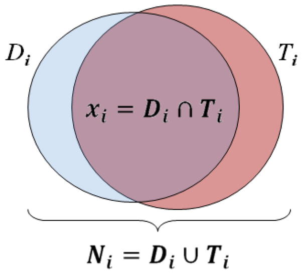
We assumed a specific ROI structure was delineated using a segmentation method on a total of M data sets and a reference ROI was available for each data set. The overlap of the segmented ROI and the reference ROI was evaluated to measure the segmentation performance. Let D_i, i = 1, …, M, denote the segmentation decision and T_i, i = 1, …, M, denote the ground truth for each data set. We define N_i, i = 1, …, M, as the total number of voxels that are assigned an object value of 1 either by the segmentation decision map or by the ground truth image and x_i, i = 1, …, M, as the number of voxels assigned a value of 1 by both the segmentation decision map and the ground truth image. Figure 1 illustrates the definition of N_i and x_i. Let y denote the underlying performance of the segmentation algorithm. This variable is unobservable and could be regarded as a random variable. Let Y = {y_i: i = 1, …, M} be the underlying performance of the method applied to the M observations; we assume that each y_i is independent and identically distributed (i.i.d.). Let X = {x_i: i = 1, …, M} denote the collection of x_i and N = {N_i: i = 1, …, M} denote the collection of N_i. We can model X as a random vector whose elements are statistically independent, where x_i is drawn from a binomial distribution with parameters N_i and y_i as

Figure 1.

Illustration of the volume overlap of auto-segmented ROI [D_i] and manual reference ROI (the ground truth [T_i]), and the definition of N_i and x_i.

$$\mathit{X}~f(\mathit{X}\mid \mathit{N},\mathit{Y})=\prod _{i=1}^{M}f(x_i\mid N_i,y_i)=\prod _{i=1}^M\left(\begin{array}{c}{N}_i\\ x_i\end{array}\right)y_i^{x_i}{(1-y_i)}^{N_i-x_i}.$$ (1)

This binomial formulation assumes underlying independency of each voxel on the binary segmented images, similar to the problem formulation in simultaneous truth and performance level estimation (STAPLE) algorithm [16]. The independency assumption is reasonable because this formulation is for evaluation purpose only. The variable y_i takes values from [0,1] to indicate the performance of the segmentation algorithm applied to the ith data set, with 1 being the best performance and 0 being the worst. Eq. (1) implies that, the greater the amount of overlap between the segmented ROI and the ground truth, i.e., the value x_i is closer to N_i for i = 1, …, M, the better the performance of the testing segmentation method. Because y_i takes values from [0,1] and the Beta distribution is a conjugate prior of the binomial distribution, it is reasonable to model variable y_i with the Beta distribution, i.e.,

$$\mathit{Y}~f(\mathit{Y}\mid \alpha ,\beta )=\prod _{i=1}^{M}f(y_i\mid \alpha ,\beta )=\prod _{i=1}^M\frac{1}{B(\alpha ,\beta )}{y}_i^{\alpha -1}{(1-y_i)}^{\beta -1},$$ (2)

where α > 0 and β > 0 are unknown parameters that need to be estimated based on the given observations of the volume overlaps. B(α, β)is the Beta function used as the normalization constant in Eq. (2):

$$B(\alpha ,\beta )={\int }_0^1{t}^{\alpha -1}{(1-t)}^{\beta -1}dt.$$ (3)

2.2. Parameter estimation

In the model denoted by Eqs. (1) and (2), {X, N} are the observed data and {α, β} are the parameters we need to estimate. In general, the {α, β} are regarded as the hyperparameters of the binomial distribution (1), and the generalized maximum likelihood (GML) can be applied to estimate these hyperparameters [17]. To be specific, let θ denote the set of parameters {α, β}. Then the parameter estimation problem can be formulated as

$$(\widehat{\mathit{Y}},\widehat{\mathit{\theta }})=arg\underset{(\mathit{Y},\mathit{\theta })}{max}f(\mathit{X},\mathit{Y}\mid \mathit{\theta })=arg\underset{(\mathit{Y},\mathit{\theta })}{max}f(\mathit{Y}\mid \mathit{\theta })f(\mathit{X}\mid \mathit{Y}).$$ (4)

This optimization problem can be implemented by successively maximizing with respect to θ and Y:

$$\{\begin{array}{ll}{\widehat{\mathit{\theta }}}^{(k)}\hfill & =arg\underset{\mathit{\theta }}{max}\{f({\mathit{Y}}^{(k)},\mathit{X}\mid \mathit{\theta })\}\hfill \\ {\widehat{\mathit{Y}}}^{(k+1)}\hfill & =arg\underset{\mathit{Y}}{max}\{f(\mathit{Y}\mid \mathit{X},{\mathit{\theta }}^{(k)})\}\hfill \end{array}.$$ (5)

Note that the first equation in Eq. (5) is equivalent to the following maximization problem:

$${\widehat{\mathit{\theta }}}^{(k)}=arg\underset{\mathit{\theta }}{max}\{f({\mathit{Y}}^{(k)}\mid \mathit{\theta })\}.$$ (6)

This can be interpreted as a maximum likelihood (ML) estimate of θ if Y^(k) could be considered as samples of the prior distribution in Eq. (2). The ML estimation for the parameters of the Beta distributions has been studied extensively [18–20]. A closed-form solution does not exist. A common alternative is to estimate the parameters using the method of moments [21]. Using this method, we have the following updated equations for parameters α and β:

$$\{\begin{array}{rr}\hfill {\alpha }^{(k)}=& \hfill {\overline{y}}^{(k)}\left[\frac{{\overline{y}}^{(k)}(1-{\overline{y}}^{(k)})}{v^{(k)}}-1\right]\\ \hfill {\beta }^{(k)}=& \hfill (1-{\overline{y}}^{(k)})\left[\frac{{\overline{y}}^{(k)}(1-{\overline{y}}^{(k)})}{v^{(k)}}-1\right]\end{array},$$ (7)

where

$${\overline{y}}^{(k)}=\frac{1}{M}\sum _{i=1}^M{y}_i^{(k)},v^{(k)}=\frac{1}{M}\sum _{i=1}^M{\left(y_i^{(k)}-{\overline{y}}^{(k)}\right)}^2.$$ (8)

To estimate Y in Eq. (5), we need to first compute the probability density function for the posterior distribution, f(Y|X, θ), i.e.,

$$\begin{array}{l}f(\mathit{Y}\mid \mathit{X},\mathit{\theta })=\frac{f(\mathit{Y}\mid \mathit{X},\mathit{\theta })}{f(\mathit{X}\mid \mathit{\theta })}=\prod _{i=1}^{M}f(y_i\mid x_i,\alpha ,\beta )\\ =\prod _{i=1}^M\frac{1}{B(x_i+\alpha ,N_i-x_i+\beta )}{y}_i^{x_i+\alpha -1}{(1-y_i)}^{N_i-x_i+\beta -1}.\end{array}$$ (9)

Eq. (9) shows that the posterior is also a Beta distribution but with parameters {x_i + α, N_i − x_i + β} for each observed data set. By taking the derivative of Eq. (9) with respect to y_i, i = 1, …, M, given the knowledge of θ^(k), we can obtain the updated equations for the performance values Y as

$$y_i^{(k+1)}=\frac{x_i+{\alpha }^{(k)}-1}{N_i+{\alpha }^{(k)}+{\beta }^{(k)}-2},i=1,\dots ,M.$$ (10)

Eqs. (7), (8), and (10) constitute an iterative procedure to estimate the parameters θ = {α, β} as well as the hidden performance values Y. The initialization for the iterative procedure can be estimated by applying the ML estimator to Eq. (1) with the assumption that y_i is deterministic. Therefore,

$$y_i^{(0)}=\frac{x_i}{N_i},i=1,\dots ,M.$$ (11)

Eq. (11) is equivalent to assuming α⁽⁰⁾ = β⁽⁰⁾ = 1, i.e., the prior distribution of the underlying performance is uniform over [0,1], the completely uninformative case. By observing Eq. (11), we can see that the initial performance is equivalent to the union volume overlap index, i.e., the Jaccard coefficient [22].

The estimation given by Eqs. (7), (8), and (10) may be unstable or over sensitive when the observations do not well distribute. In this situation, the estimated $y_i^{(k)}$, i = 1, …, M, from Eq. (10) converges to the mean of $y_i^{(k)}$ so that the variance in Eq. (8), v^(k), becomes very small. This will cause numerical instability when estimating α^(k) and β^(k) in Eq. (7). Should this situation happen, we will use $y_i^{(0)}$ in Eqs. (7) and (8) to estimate {α, β} directly, instead of going through the iterative estimation. However, in real cases, this situation normally will not happen.

2.3. Statistical performance evaluation

In our data model, the performance of a segmentation method is represented by a random variable y, and the final estimates Y = {y_i:i = 1, …, M} can be viewed as the samples of the underlying performance y when the method is applied to the M data sets. As mentioned previously, y follows the Beta distribution with a probability density function (PDF) of

$$f(y\mid \alpha ,\beta )=\frac{1}{B(\alpha ,\beta )}{y}^{\alpha -1}{(1-y)}^{\beta -1},$$ (12)

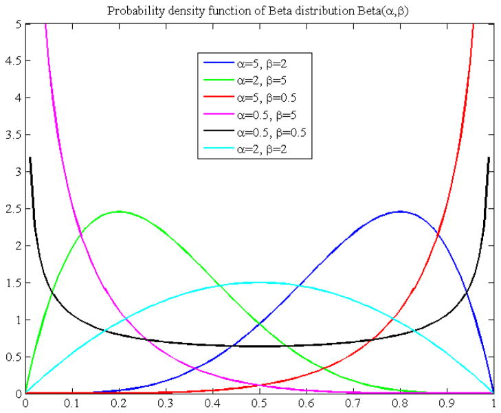
where α and β are the parameters estimated on the basis of the observed data using the method described in section 2.2. The PDF in Eq. (12) exemplifies the distribution of the performance values over [0, 1]. We refer to this PDF as the statistical performance profile (SPP) for the given segmentation method. For different data sets or different ROIs in the same data sets, the SPP could be different for a same segmentation method. The SPP can also be graphically displayed with a curve, which intuitively illustrates the distribution of the segmentation performance values. Figure 2 shows some examples of the SPP, i.e. the PDF of the Beta distribution. Using the SPP, the performance of a given method can be easily visualized and the performance of different methods can be easily compared.

Figure 2.

Probability density function of Beta distribution with different parameters (α, β). The pdf plot shows the distribution of performance values in the interval [0, 1].

The expected performance score (mean) for a given method based on the M observations can be given by the expectation of y as

$$E(y\mid \alpha ,\beta )=\frac{\alpha }{\alpha +\beta }.$$ (13)

The standard deviation (SD) of the distribution is another important measure for the performance evaluation and may be related to the robustness of the segmentation performance,

$$SD(y\mid \alpha ,\beta )=\sqrt{\frac{\alpha \beta }{{(\alpha +\beta )}^2(\alpha +\beta +1)}}.$$ (14)

The performance score obtained when the method is applied to a new data set with prior knowledge of the Beta distribution may also be of interest. Assume the ROI overlap (N, x) for the new data set is observed. Then the posterior distribution of the performance would be

$$y\mid x~f(y\mid x,\alpha ,\beta )=\frac{1}{B(x+\alpha ,N-x+\beta )}{y}^{x+\alpha -1}{(1-y)}^{N-x+\beta -1}.$$ (15)

With this observation, the performance score for this data set would be

$$E(y\mid x,\alpha ,\beta )=\frac{\alpha +x}{\alpha +\beta +N}.$$ (16)

This value can be viewed as a performance score rectified from the Jaccard coefficient by considering the prior knowledge learned from the training data with properties similar to the new data set.

3. Results

In this section, we will first use the Monte Carlo simulation to justify the iterative parameter estimation method described in section 2.2. Then we will present results from both a simulation study and a clinical study to demonstrate the efficacy of our statistical modeling method. Specifically, we applied the SPP to evaluate an atlas-based segmentation method using deformable image registration. In our experiments, we performed deformable image registration [6] to obtain a vector field characterizing the mapping from the atlas image to the testing image. This vector field was then used to transfer the well-defined ROI structures on the atlas to the corresponding positions on the testing image for segmentation.

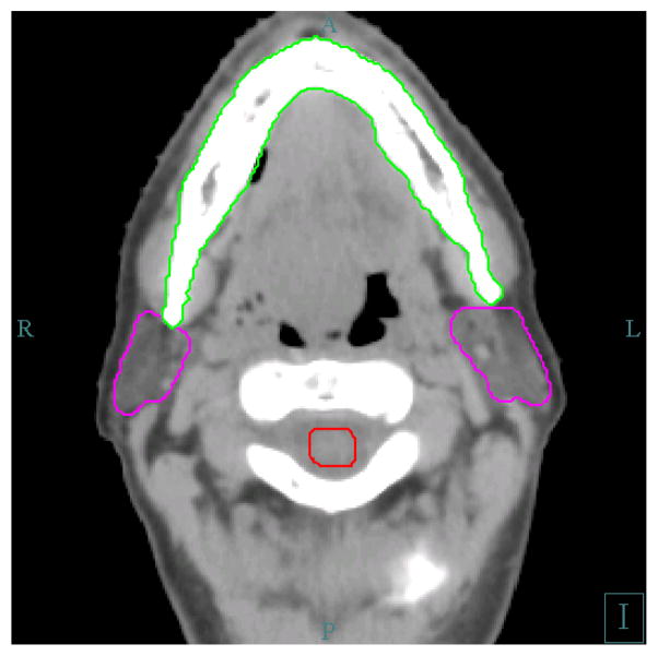
The data used in our study are the computed tomography (CT) images of head and neck cancer patients. The structures of interest are the bilateral parotid glands. Parotid gland is one of the most important organs to be avoided during the head and neck radiotherapy. The delineation of parotid gland is not easy due to the low contrast of this organ with its surrounding tissues, such as muscle and skins, on the CT image. The pitch rotation of the head may also add difficulty to exactly locate the parotid glands on the axial slices of the CT image. Figure 3 shows some important structures on an axial CT slice that are normally contoured for head and neck radiotherapy.

Figure 3.

Some normal structures delineated for head and neck radiotherapy. The left and right parotid glands are in magenta color, the mandible is in green color, and the spinal cord is in read, surrounded by cervical vertebrae.

3.1. Accuracy of parameter estimation

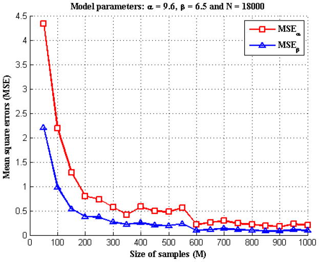
To verify the accuracy of parameter estimation described in section 2.2, we performed the following Monte Carlo simulation. In particular, we were interested in how the number of samples, M, affected the parameter estimation. To perform the simulation, we assumed the data model had known values of α,β, and N (of size M) and then generated 100 realizations of X using Eqs. (1) and (2). We ran the iterative algorithm described in section 2.2 to get α̂ and β̂, the estimation of parameters α and β, respectively. Then we calculated the mean square errors (MSEs) of the estimation, i.e., E((α̂ − α)²) and E((β̂ − β)²) based on the 100 simulations. We varied the value M and repeated the simulation to record the MSEs at different numbers of samples for comparison. Figure 4 illustrated an example with α = 9.6, β = 6.5 and a constant number of 18000 for each N_i, (i = 1, …, M). We chose various values of M from 50 to 1000 and calculated the MSEs for α and β, respectively. In figure 4, for both α and β, the estimation error decreased as the sample size M increased. When the sample size was less than 300, the parameter estimation was biased by the variations existing in the samples thus resulting to estimation error. When the sample size was over 300, the error became very small; when the sample size further increased to over 600, we were able to obtain an estimation that was quite accurate.

Figure 4.

The MSEs of α and β estimations for different sizes of samples.

3.2. Simulation study

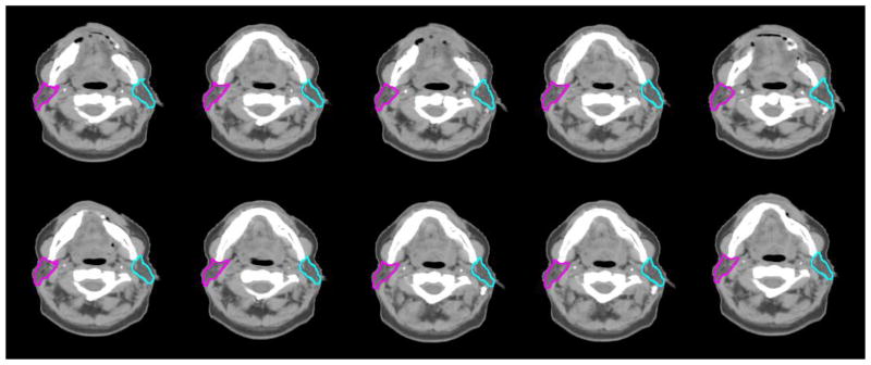
We constructed a set of deformed CT images from a reference patient with head and neck cancer; the images were obtained during a course of radiotherapy with an in-room CT scanner (Mx8000 IDT, Philips Medical Systems, Cleveland, OH). All CT scans were obtained from patient database through an institutional review board-approved protocol. Two steps were involved in creating the simulated deformed CT images: a training step and a simulation step. In the training step, we performed deformable image registration to deform the planning CT to 33 daily CTs in a treatment course to acquire 33 deformation fields that represented real changes in human anatomy. We then applied principal component analysis (PCA) to these 33 deformation fields to extract the mean deformation field and 10 most prominent modes of variation. In the simulation step, we used the mean field and 10 modes of variation as a template to generate random deformation fields, as described in a previous study [23]. The random deformation fields were then applied to the planning CT to produce a set of deformed CT images. The defined contours on the planning CT were also transformed to each deformed CT as the ground truth that would be used in the performance evaluation. We generated 600 deformed CT images. Figure 5 shows some of the simulated CTs with defined contours. Our simulation method was similar to the one proposed in a previous study [24]. Because the random deformation fields were learned from real changes in human anatomy, the simulated CT could represent realistic human subjects.

Figure 5.

Ten examples of the simulated CT images with defined left and right parotid contours. This figure shows the axial view of these images in the same slice.

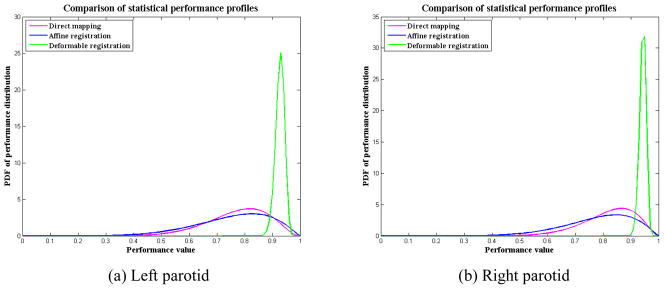
In these 600 deformed CT images, we randomly selected 300 as atlas images and the remaining 300 CTs were used as testing images to form 300 pairs of atlas-testing image sets. We preformed the registration between the atlas and testing images for each pair and transformed the contours on the atlas image to the testing image automatically. We examined the bilateral parotid glands because they are critical structures to spare in head and neck radiotherapy. Two registration algorithms were used to generate the automatic delineated contours. One registration algorithm was the linear registration using the centered affine transformation with an intensity similarity metric, which was implemented in ITK [25]. The other registration algorithm was the deformable registration using the dual-force “Demons” algorithm [6]. We also directly mapped the atlas contours to testing image sets without performing any registration. We computed the SPP for each contour mapping method and demonstrated how SPP could easily be used to compare the performance of different approaches. The estimated SPP parameters are presented in table 1, and the SPPs are illustrated in figure 6. From figure 6, it is easy to see that the deformable registration performed much better than the affine registration in this testing. This result is not surprising because the simulated data were generated with random local deformation instead of global transformation. The global affine registration was not able to recover the local deformation. Because the parotid glands are small relative to the entire head-and-neck region, affine registration may be able to improve the registration for the entire image but may not result in good registration in the parotid gland region. This fact may explain our observation of a wider spread of SPP for affine registration than for direct mapping. In other words, the affine registration was not robust when we used it to register the parotid glands. The larger SD in table 1 also showed this point. The SPP for the deformable registration had a narrow and sharp outline, which demonstrated a robust good performance.

Table 1.

Estimated parameters of the statistical performance profiles for direct mapping, affine registration, and deformable registration methods. These parameters were estimated from 50 samples of the simulated data (M=50).

Methods	Left parotid				Right parotid
	α	β	Mean	SD	α	β	Mean	SD
Direct mapping	10.71	3.17	0.772	0.109	12.52	2.77	0.819	0.096
Affine registration	6.98	2.25	0.756	0.134	8.05	2.28	0.780	0.123
Deformable registration	239.25	18.83	0.927	0.016	366.85	22.08	0.943	0.012

Figure 6.

SPPs for direct mapping, affine registration, and deformable registration methods when they are applied to (a) left parotid contours and (b) right parotid contours. For better performance, the SPP curve should be narrow and sharp, and towards the high performance value. In this illustration, deformable registration shows a better performance than affine registration and direct mapping.

3.3. Clinical study

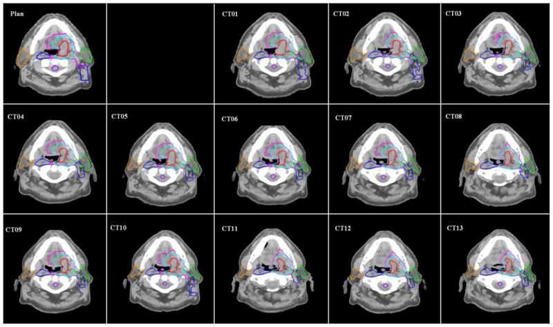
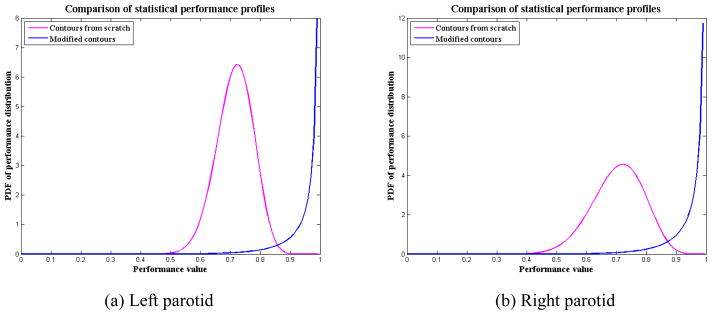
In this clinical study, we demonstrated the capability of our SPP to show the intra-observer variability in clinical contouring. CT images for 10 head and neck cancer patients who had undergone three CT scans weekly using an in-room CT scanner were evaluated for the accuracy of the contours that were automatically propagated from the planning CT image. Each of these 10 patients had undergone 11–14 daily CT scans, and a total of 122 CT scans were evaluated. One physician contoured each daily CT from scratch and modified deformed contours that were propagated from the planning CT. The automatic contour propagation was implemented with deformable registration using the dual-force “Demons” algorithm [6]. Figure 7 shows an example of the auto-propagated contours for one of the head-and-neck cancer patients. Some of the most important contours for radiotherapy are displayed, such as the primary targets, clinical target volumes (CTVs) of three risk levels, parotid glands, and spinal cord. For each patient, the deformed contours were compared with both the physician-drawn contours and the physician-modified contours for performance evaluation. We computed the SPPs for the high-risk CTV and both parotid gland contours. CTV were not contoured from scratch due to its high variations across the treatment course. Table 2 shows the estimated parameters, and figure 8 compares the SPPs of “contours from scratch” and “modified contours” for the left and right parotid glands.

Figure 7.

Auto-propagated contours for one patient with head-and-neck cancer. Original contours were drawn on the “Plan” CT and then were transformed automatically using deformable image registration to the daily CT images (“CT1”, “CT2”, …, “CT13”).

Table 2.

Estimated parameters of the SPPs for contours from scratch and for modified contours. “Contours from scratch” represents the SPP by comparing the deformed contours with the physician-drawn contours. “Modified contours” represents the SPP by comparing the deformed contours with the physician-modified contours. These parameters were estimated from the 122 daily CT scans.

ROIs	Contours from scratch				Modified contours
	α	β	Mean	SD	α	β	Mean	SD
Left parotid	37.67	15.04	0.715	0.062	7.32	0.11	0.986	0.041
Right parotid	19.01	7.96	.705	0.086	7.69	0.19	0.976	0.052
CTV					25.42	1.64	0.939	0.045

Figure 8.

SPPs for contours from scratch and for modified contours. In this illustration, the “modified contours” shows a much better performance than the “contours from scratch”.

Parotid glands are difficult to delineate due to their low contrast to surrounding tissue and high variability. Even experienced physicians may produce different contours if they are asked to independently contour the same anatomy twice. The SPPs for “contours from scratch” in table 2 or figure 8 demonstrate this point. The SPPs showed a mean segmentation performance of 0.71 with averaged standard deviation of 0.07 for both parotid contours. Figure 8 also showed the performance values were mostly distributed in [0.5, 0.9], and the probability of performance value above 0.90 was nearly 0. This demonstrated the high intra-observer variability in contouring the CT scans of patients with head and neck cancer.

The same physician who did the previous contouring was also asked to modify the deformed contours to generate a set of clinically acceptable contours. The SPPs for the “modified contours” showed a much higher performance, with a mean value around 0.98 and standard deviation of 0.05. Because the mean value is very close to the right boundary 1.0, the distribution significantly skews to the left so that the PDF curve peaks at the boundary, as shown in figure 8 of the curves for the modified contours. This illustrates that the performance values most likely distribute around 1.0. Actually, the distribution of performance values was mostly in [0.7, 1.0], and the probability of performance value above 0.99 was around 80% for both parotid glands. The physician also modified the deformed CTV contours. The SPP showed a mean performance for modified CTV contours as 0.94, with 50% probability of these contours having a performance value above 0.95. This indicates that the auto-propagated contours matched well with the physician’s judgment and the intra-observer variability was significantly reduced when the physician modified contours from a reference. By comparing the SPPs of the “contours from scratch” and the “modified contours”, we concluded that the auto-propagated contours were very helpful in reducing the observer variability in clinical contouring practice. This, on the other hand, also demonstrated that the observer variability in the manual reference contours had a great impact on the evaluation of auto-segmentation.

4. Discussion

We have demonstrated an efficient statistical modeling method to evaluate the accuracy of anatomy segmentation with a focus on applications for head and neck radiotherapy. This method takes advantage of a parameterized statistical model, and the model parameters are estimated from a set of observations. The number of the observations (i.e., the samples) has a great impact on the estimated parameters. In our Monte Carlo study described in section 3.1, we found the estimation was generally not subject to the sample variations and was relatively accurate when the number of samples was over 300. With a limited number of data samples, the variance in the data may affect the estimated performance profile. In general, the SPP may be biased if the data collection is limited to specific cases, such as intra-patient contour propagation or contours produced by one physician only. However, the estimated SPP was still meaningful since it would reflect the estimated performance for only the given testing samples. It is very important to specify the testing data accurately when discussing the SPP. Furthermore, to better characterize segmentation performance for a specific treatment site, such as the head and neck, one needs to collect a variety of data that are typical for that site in clinical practice and pick representative ROIs to generate the SPPs. The collection of the clinical data to generate a benchmark database therefore is very important to thoroughly evaluate a given segmentation method.

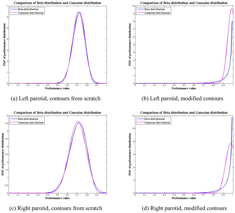
We also compared our SPP of the Beta distribution against the statistical analysis based on the assumption of a Gaussian distribution. We used the SPPs for parotid glands in our clinical study (Section 3.3) as an example to illustrate the difference between Gaussian and Beta distributions. Table 3 lists the means and SDs of the Beta distribution and the Gaussian distribution for both parotid glands using the two contouring methods, contouring from scratch and modifying deformed contours. The means and SDs of the Gaussian distribution were computed based on the samples of observed volume overlap, i.e., the Jaccard coefficient $\frac{x_i}{N_i}$, i = 1, …, M. We found that the means and SDs of the Beta distribution and the Gaussian distribution were similar. This was not surprising because we used the method of moments to estimate the parameters for the Beta distribution, which forced the means and SDs of the Beta distribution to be the same as those of the Gaussian distribution. However, the distribution could be quite different when the sample mean is close to 1 for the cases of modified contours. Figures 9(a) and (c) show that the Beta distribution is very close to the Gaussian distribution for the contouring-from-scratch method. Although Gaussian distribution looks slightly sharper in Figure 9(c), it does not necessarily mean that Gaussian distribution is better than Beta distribution. In this situation, further study is required to determine which model is better, such as the monotonic hypothesis testing [26, 27] discussed later in this section. However, figures 9(b) and (d) show that the distributions are quite different for the modifying-deformed-contours method. In this situation, the Beta distribution is more appropriate to approximate the actual performance distribution than the Gaussian distribution because the Gaussian distribution is incomplete in the range of [0, 1].

Table 3.

Means and SDs for the Beta distribution and the Gaussian distribution for the observations of parotid contour overlap described in section 3.2.

		Contours from scratch		Modified contours
		Mean	SD	Mean	SD
Left Parotid	Beta distribution	0.715	0.062	0.986	0.041
	Gaussian distribution	0.715	0.062	0.985	0.041
Right Parotid	Beta distribution	0.705	0.086	0.976	0.052
	Gaussian distribution	0.705	0.087	0.976	0.052

Figure 9.

Comparison of the Beta distribution and Gaussian distribution for the parotid contours described in section 3.3. For the contouring from scratch, the performance distribution is similar for both Beta and Gaussian distribution; for modifying contours method, the Beta distribution is better than the Gaussian distribution since the effective range of Gaussian distribution is beyond the interval [0, 1].

Another important aspect of our quantitative evaluation study was our attempt to verify whether a proposed objective evaluation measure accurately predicts human perception. Human perceptual evaluation is generally accurate if the subjective human tests are performed correctly; however, subjective human tests are inconvenient, expensive, and time-consuming. The performance may also depend greatly on the experience of the persons involved in the testing. Therefore, it is desirable to investigate a quantitative measure that can accurately “predict” subjective human perception. Because understanding of the human visual system (HVS) is incomplete, this type of investigation is quite difficult. In our previous study, we developed a monotonic correlation method [26] and a diffuse prior monotonic likelihood ratio (DPMLR) method [27] to analyze image quality for image fusion. In those studies, we evaluated how well the fused image quality measures indicated the effectiveness of human perception of targets of interest in fused imagery to determine effective quantitative evaluation measurements for image fusion algorithms. The key in those studies was to create a data model for evaluation purposes and then use hypothesis testing to relate the intrinsic human perceptual evaluation to the quantitative measures. In the present work, we have proposed a statistical model, which can be used for this correlation analysis. In our future studies, we will devise an experiment to determine how well this proposed measurement relates to clinical experts’ decision, and ultimately to guide the clinicians in selecting segmentation methods for radiotherapy.

5. Conclusion

We have developed a statistical modeling method for evaluating different segmentation algorithms. The efficiency of this method has been demonstrated in head and neck radiotherapy. A statistical model was developed based on Beta distribution and statistical inferences of a set of observations. We derived the SPP from the model using the generalized maximum likelihood approach to characterize the distribution of performance values. The SPP was able to differentiate the performance of segmentation in the presence of observer variability and quality of the images and provided a graphical visualization of the segmentation performance. We validated this method in both simulation studies and clinical data.

References

- 1.Ezzell GA, Galvin JM, Low D, Palta JR, Rosen I, Sharpe MB, Xia P, Xiao Y, Xing L, Yu CX. Guidance document on delivery, treatment planning, and clinical implementation of IMRT: Report of the IMRT subcommittee of the AAPM radiation therapy committee. Medical Physics. 2003;30:2089–2115. doi: 10.1118/1.1591194. [DOI] [PubMed] [Google Scholar]
- 2.Mackie TR, Kapatoes J, Ruchala K, Lu W, Wu C, Olivera G, Forrest L, Tome W, Welsh J, Jeraj R, Harari P, Reckwerdt P, Paliwal B, Ritter M, Keller H, Fowler J, Mehta M. Image guidance for precise conformal radiotherapy. International Journal of Radiation Oncology * Biology * Physics. 2003;56:89–105. doi: 10.1016/s0360-3016(03)00090-7. [DOI] [PubMed] [Google Scholar]
- 3.Cozzi L, Fogliata A, Bolsi A, Nicolini G, Bernier J. Three-dimensional conformal vs. intensity-modulated radiotherapy in head-and-neck cancer patients: Comparative analysis of dosimetric and technical parameters. International Journal of Radiation Oncology * Biology * Physics. 2004;58:617–624. doi: 10.1016/j.ijrobp.2003.09.059. [DOI] [PubMed] [Google Scholar]
- 4.Chao KSC, Bhide S, Chen H, Asper J, Bush S, Franklin G, Kavadi V, Liengswangwong V, Gordon W, Raben A, Strasser J, Koprowski C, Frank S, Chronowski G, Ahamad A, Malyapa R, Zhang L, Dong L. Reduce in Variation and Improve Efficiency of Target Volume Delineation by a Computer-Assisted System Using a Deformable Image Registration Approach. International Journal of Radiation Oncology * Biology * Physics. 2007;68:1512–1521. doi: 10.1016/j.ijrobp.2007.04.037. [DOI] [PubMed] [Google Scholar]
- 5.Stapleford LJ, Lawson JD, Perkins C, Edelman S, Davis L, McDonald MW, Waller A, Schreibmann E, Fox T. Evaluation of Automatic Atlas-Based Lymph Node Segmentation for Head-and-Neck Cancer. International Journal of Radiation Oncology * Biology * Physics. 2010;77:959–966. doi: 10.1016/j.ijrobp.2009.09.023. [DOI] [PubMed] [Google Scholar]
- 6.Wang H, Dong L, Lii MF, Lee AL, de Crevoisier R, Mohan R, Cox JD, Kuban DA, Cheung R. Implementation and validation of a three-dimensional deformable registration algorithm for targeted prostate cancer radiotherapy. International Journal of Radiation Oncology * Biology * Physics. 2005;61:725–735. doi: 10.1016/j.ijrobp.2004.07.677. [DOI] [PubMed] [Google Scholar]
- 7.Reed VK, Woodward WA, Zhang L, Strom EA, Perkins GH, Tereffe W, Oh JL, Yu TK, Bedrosian I, Whitman GJ, Buchholz TA, Dong L. Automatic Segmentation of Whole Breast Using Atlas Approach and Deformable Image Registration. International Journal of Radiation Oncology * Biology * Physics. 2009;73:1493–1500. doi: 10.1016/j.ijrobp.2008.07.001. [DOI] [PMC free article] [PubMed] [Google Scholar]
- 8.Lu WG, Olivera GH, Chen Q, Chen ML, Ruchala KJ. Automatic re-contouring in 4D radiotherapy. Physics in Medicine and Biology. 2006;51:1077–1099. doi: 10.1088/0031-9155/51/5/002. [DOI] [PubMed] [Google Scholar]
- 9.Commowick O, Gregoire V, Malandain G. Atlas-based delineation of lymph node levels in head and neck computed tomography images. Radiotherapy and Oncology. 2008;87:281–289. doi: 10.1016/j.radonc.2008.01.018. [DOI] [PubMed] [Google Scholar]
- 10.Haas B, Coradi T, Scholz M, Kunz P, Huber M, Oppitz U, Andre L, Lengkeek V, Huyskens D, vanEsch A, Reddick R. Automatic segmentation of thoracic and pelvic CT images for radiotherapy planning using implicit anatomic knowledge and organ-specific segmentation strategies. Physics in medicine and biology. 2008;53:1751–1771. doi: 10.1088/0031-9155/53/6/017. [DOI] [PubMed] [Google Scholar]
- 11.Zhang YJ. A survey on evaluation methods for image segmentation. Pattern Recognition. 1996;29:1335–1346. [Google Scholar]
- 12.Wang H, Garden AS, Zhang L, Wei X, Ahamad A, Kuban DA, Komaki R, O’Daniel J, Zhang Y, Mohan R, Dong L. Performance Evaluation of Automatic Anatomy Segmentation Algorithm on Repeat or Four-Dimensional Computed Tomography Images Using Deformable Image Registration Method. International Journal of Radiation Oncology * Biology * Physics. 2008;72:210–219. doi: 10.1016/j.ijrobp.2008.05.008. [DOI] [PMC free article] [PubMed] [Google Scholar]
- 13.Sims R, Isambert A, Gregoire V, Bidault F, Fresco L, Sage J, Mills J, Bourhis J, Lefkopoulos D, Commowick O, Benkebil M, Gregoire M. A pre-clinical assessment of an atlas-based automatic segmentation tool for the head and neck. Radiotherapy and oncology : Journal of the European Society for Therapeutic Radiology and Oncology. 2009;93:474–478. doi: 10.1016/j.radonc.2009.08.013. [DOI] [PubMed] [Google Scholar]
- 14.Teguh DN, Levendag PC, Voet PWJ, Al-Mamgani A, Han X, Wolf TK, Hibbard LS, Nowak P, Akhiat H, Dirkx MLP, Heijmen BJM, Hoogeman MS. Clinical Validation of Atlas-Based Auto-Segmentation of Multiple Target Volumes and Normal Tissue (Swallowing/Mastication) Structures in the Head and Neck. International Journal of Radiation Oncology * Biology * Physics. 2010:1–8. doi: 10.1016/j.ijrobp.2010.07.009. In Press. [DOI] [PubMed] [Google Scholar]
- 15.Dice LR. Measures of the Amount of Ecologic Association Between Species. Ecology. 1945;26:297–302. [Google Scholar]
- 16.Warfield SK, Zou KH, Wells WM. Simultaneous truth and performance level estimation (STAPLE): an algorithm for the validation of image segmentation. IEEE Transactions on Medical Imaging. 2004;23:903–921. doi: 10.1109/TMI.2004.828354. [DOI] [PMC free article] [PubMed] [Google Scholar]
- 17.Mohammad-djafari A. On the estimation of hyperparameters in Bayesian approach of solving inverse problems. International Conference on Acoustics, Speech, and Signal Processing (ICASSP’93); Minneapolis, MN. 1993. pp. 495–498. [Google Scholar]
- 18.Hahn GJ, Shapiro SS. Statistical Models in Engineering. New York, NY: John Wiley & Sons, Inc; 1994. [Google Scholar]
- 19.Nguyen TT. Maximum Likelihood Estimators of the Parameters in a Beta Distribution. In: Gupta AK, Nadarajah S, editors. Handbook of Beta Distribution and Its Applications. New York, NY: CRC Press; 2004. pp. 229–235. [Google Scholar]
- 20.Johnson NL, Kotz S, Balakrishnan N. Continuous Univariate Distributions. 2. II. New York, NY: John Wiley & Sons, Inc; 1995. [Google Scholar]
- 21.Bain LJ, Engelhardt M. Introduction to Probability and Mathematical Statistics. 2. Pacific Grove, CA: Duxbury Press; 2000. [Google Scholar]
- 22.Jaccard P. The Distribution of the Flora in the Alpine Zone. New Phytologist. 1912;11:37–50. [Google Scholar]
- 23.Cootes TF, Hill A, Taylor CJ, Haslam J. Use of active shape models for locating structures in medical images. Image and Vision Computing. 1994;12:355–365. [Google Scholar]
- 24.Xue Z, Shen D, Karacali B, Stern J, Rottenberg D, Davatzikos C. Simulating deformations of MR brain images for validation of atlas-based segmentation and registration algorithms. NeuroImage. 2006;33:855–866. doi: 10.1016/j.neuroimage.2006.08.007. [DOI] [PMC free article] [PubMed] [Google Scholar]
- 25.Ibanez L, Schroeder W, Ng L, Cates J. The ITK Software Guide. 2. Clifton Park, NY: Kitware Inc; 2005. [Google Scholar]
- 26.Kaplan LM, Burks SD, Blum RS, Moore RK, Quang N. Analysis of Image Quality for Image Fusion via Monotonic Correlation. IEEE Journal of Selected Topics in Signal Processing. 2009;3:222–235. [Google Scholar]
- 27.Wei C, Kaplan LM, Burks SD, Blum RS. Diffuse Prior Monotonic Likelihood Ratio Test for Evaluation of Fused Image Quality Measures. IEEE Transactions on Image Processing. 2011;20:327–344. doi: 10.1109/TIP.2010.2060344. [DOI] [PubMed] [Google Scholar]