Analysis of Multidimensional G-Quadruplex Melting Curves

Abstract

Multidimensional “3D” melting curves for G-quadruplexes are obtained by recording whole spectra (absorbance, CD, fluorescence) as a function of temperature rather than the common approach of recording the spectral response to temperature at a single wavelength. 3D melting curves are richer in information, and can be used to enumerate the number of significant species and intermediates states required to properly analyze the thermal denaturation reaction to obtain thermodynamic information. This unit describes the application of the method of singular value decomposition to the analysis of 3D melting data obtained for G-quadruplex structures, and how the results of such an analysis can be used to provide a more complete characterization of the mechanism of quadruplex unfolding.

Introduction

G-quadruplexes are a family of nucleic acids structures of intense current interest both because of their potential functional importance and their emergence as attractive drug targets. G-rich sequences can spontaneously form a variety of G-quadruplex structures, the cores of which feature stacks of planar guanine quartets in a variety of orientations and arrangements. Unit 17.2 provides an overview of G-quadruplex structures and of methods commonly used for their characterization.

In addition to high-resolution structural characterization provided by NMR (Unit 7.2) or X-ray crystallography (Unit 7.13), it is essential to understand the thermodynamics and kinetics of G-quadruplex folding and unfolding to gain a fundamental understanding of their stability and reactivity. Thermal denaturation, with spectroscopic detection, offers one tried and true approach for measuring the stability of nucleic acid structures. Unit 7.3 describes protocols for UV melting studies of nucleic acids in general, and Unit 17.1 describes UV melting studies of G-quadruplexes in particular. In both of these units, thermal denaturation methods with optical detection at a single wavelength are described, followed by analysis using two-state models to obtain thermodynamic parameters for the unfolding reaction. Two-state models assume that only folded and unfolded species exist in equilibrium, with no intermediate states along the unfolding pathway that are significantly populated. While the two-state assumption is certainly a reasonable starting point for analysis and is analytically convenient, it does require experimental validation and justification. The multidimensional “3D” melting approach we describe in this unit provides a means for rigorous testing of the two-state assumption, and for the identification of intermediate species that may exist that must be accounted for in the unfolding reaction mechanism.

The two-state assumption may be readily tested by acquiring thermal denaturation by different types of spectroscopy each at a single wavelength (absorbance, circular dichroism, fluorescence) or by calorimetry (Unit 7.4). Long ago, Lumry and coworkers (Lumry and Biltonen, 1966) showed that denaturation transition curves obtained by different biophysical approaches should superimpose if the two-state melting assumption were valid; lack of superposition of transition curve is inconsistent with a simple two-state denaturation mechanism. More recently, a dual wavelength parametric test was proposed as a test of the two-state assumption (Wallimann et al., 2003). In this test, denaturation transition curves are measured at two wavelengths. If the two-state assumption is valid, the spectral data at the two wavelengths should be linearily correlated. Deviations from strict linearity indicate that the data are inconsistent with the two-state assumption. Both of these approaches offer simple tests of the two-state model, but “3D melting” offers an even more powerful and informative approach.

For the 3D melting approach, the thermal denaturation experiment is conducted as usual (Units 7.3, 17.1), but instead of collecting spectroscopic data at a single-wavelength, a more complete spectrum over a range of wavelengths is collected at each temperature. This is easily done with any modern computer-controlled instrument, especially with spectrometers that feature diode array detection systems. 3D melting can be done using UV absorbance, circular dichroism or fluorescence detection. Since the acquisition of 3D thermal denaturation data is practically the same as is described in detail in Units 7.3 & 17.1, this unit will focus on the analysis and interpretation of the 3D dataset. The method of singular value decomposition (SVD) (DeSa and Matheson, 2004; Hendler and Shrager, 1994; Henry and Hofrichter, 1992) provides a rigorous, model-free analytical method for the characterization of 3D melting sets (Haq et al., 1997). The results of an SVD analysis can then be fit to equilibrium models to obtain mechanistic and thermodynamic information (Greenfield, 2006). This unit will describe how this might be done using available software packages.

Overview of SVD analysis

In a 3D melting experiment, spectra over a desired wavelength range are collected as a function of temperature, as exemplified by the data in Figure 3A. Such data may be converted in matrix form to provide the r × c matrix D, the elements of which are absorbance values (or other spectral responses) arranged with rows (r) corresponding to wavelengths and columns (c) corresponding to temperatures (fig. 1B). A plot of a single column vector would yield an absorbance spectrum at a particular temperature (fig. 1C), while plot of a row vector would correspond to the familiar melting curve obtained at a single wavelength (fig. 1D).

Figure 3.

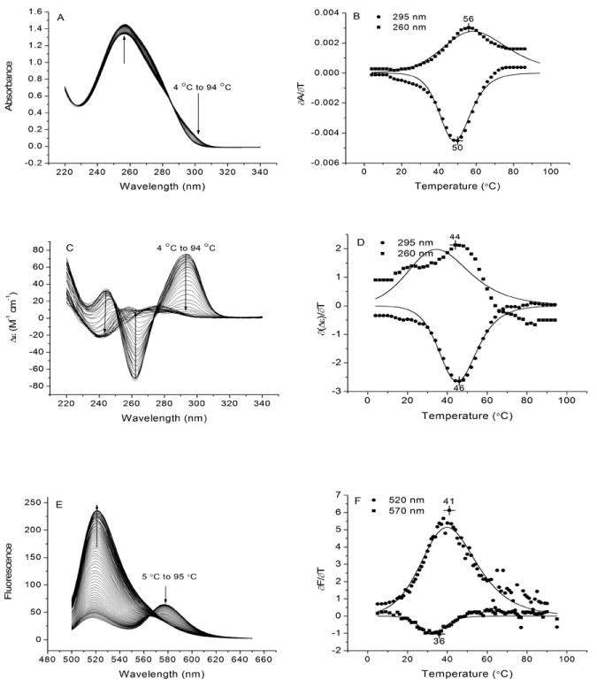
Temperature-dependence of the UV absorption, CD and FRET properties of the oligonucleotide d[A(GGGTTA)₃] (143D) which forms a quadruplex structure in 50 mM NaCl. Panels A, C and E show spectroscopic measurements for each method as a function of increasing temperature. The arrows represent the direction of the signal change as the temperature is increased. Panels B, D and F compare the corresponding first derivative of the signal with respect to temperature at the indicated wavelengths. The points in Panels A, C & E were obtained from the raw data by smoothing with a 9-point, second order Savitzky-Golay filter prior to calculation of the first derivative using the program Origin 7.0. Each solid line in the derivative plot represents a non-linear least squares fit of the smoothed data points to a two-state F ↔ U mechanism described by Equation 1. Note that the data points are not well-represented by the two-state model. In addition, the apparent mid-point temperature as indicated by the number above the maximum or minimum of each curve depends both on the wavelength of observation as well as the method of measurement. Both of these factors indicate that the two-state model is unable to accurately describe the temperature-dependence of the optical signal. The absorbance and CD measurements were carried out with 143D and FRET measurements were carried out with 6-Fam-143D-Tamra. Conditions: 10 mM tetrabutyl ammonium phosphate, 50 mM NaCl, 1 mM EDTA, pH 7.0. Oligonucleotide concentrations were: 4.6 μM for the absorbance experiments, 4.7 μM for the CD experiments, and 0.1 μM for the fluorescence experiments.

Figure 1.

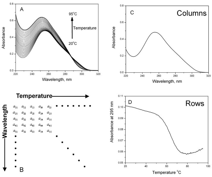
Multidimensional melting data and the structure of data sets used for analysis. (A) Examples of UV spectra as a function of temperature. (B) Structure of the data matrix constructed from multidimensional melting data. (C) Columns of the data matrix show the UV spectrum at a single temperature. (D) Rows of the data matrix show the melting curve at a single wavelength.

Singular value decomposition is a method from linear algebra for factoring a matrix. SVD has seen wide applicability in statistics and signal processing. Using SVD, the data matrix D can be factored into the product of three matrices, U, S and V:

$$\mathbf{D}={\mathbf{USV}}^{\mathbf{T}}$$

The details of the SVD computational algorithm need not (and will not) be presented here. By use of numerous available software packages (MATLAB™, Mathmatica™, for example) SVD can be done on a data matrix as a “black box” operation to yield the U, S and V matrices for analysis. This unit will focus on the interpretation and utility of these results, and will illustrate the application of SVD to multidimensional melting data.

The U matrix contains, for the case of multidimensional melting data, the so-called basis spectra, which are normalized component spectral shapes that combine to form the family of spectra in the data matrix. The S matrix is a diagonal matrix that contains the singular values, the magnitudes of which are the weights of the components. The singular values are used to initially identify the number of principal components in the data spectra. The V matrix contains the amplitude vectors as a function of the experimental variable, temperature in the case of melting data. Each significant vector has a shape reminiscent of a transition curve. The information in the U, S and V matrices is used to decide the number of significant spectral species that comprise the spectra in the data matrix D, and the number of intermediate species that must be included in any mechanistic model imposed on the data to extract thermodynamic parameters.

Figure 2 shows a flow diagram that provides an overview of the steps in the analysis of multidimensional data. Our laboratory typically uses the software MATLAB™ for this purpose, although any software package that contains the SVD function and graphics capabilities may be used. Following SVD analysis, data may be fit to obtain thermodynamic parameters. While such fitting could be implemented in MATLAB™, we find it convenient to use a second software package for that purpose, OLIS GlobalWorks™. OLIS GlobalWorks™ is purpose-designed for the analysis of multidimensional spectral data sets, and has its own SVD capability. It also allows for fitting of SVD data to selected kinetic and equilibrium thermodynamic models, as will be illustrated. Step-by-step protocols for these analyses will follow.

Figure 2.

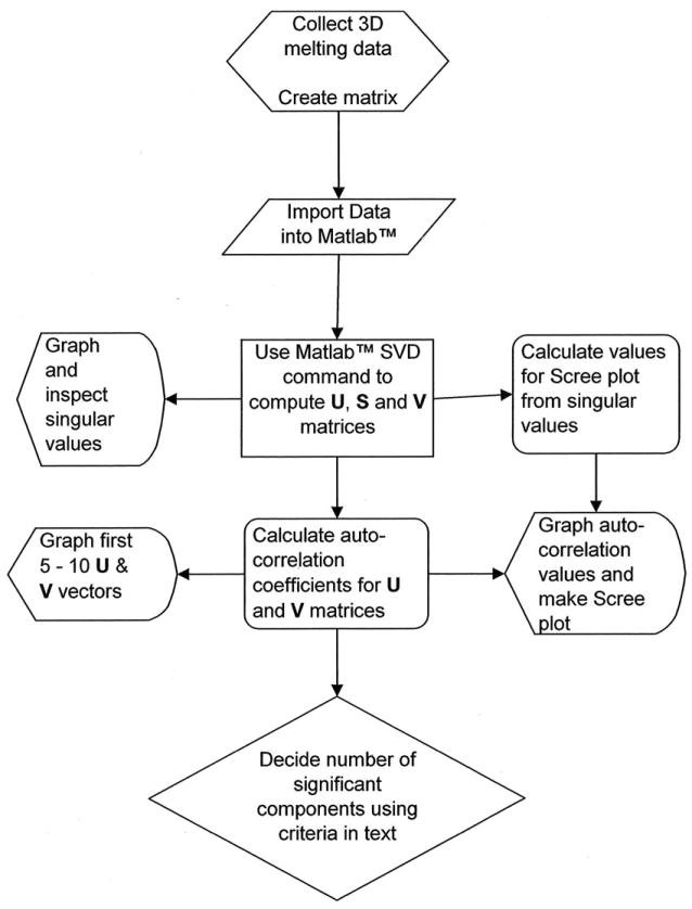
Flowchart for the analysis of multidimensional melting data.

Several comments are needed to clarify the steps shown in figure 2. The first step in the analysis of SVD data is close inspection of the singular values, the diagonal elements in the S matrix. A graph or histogram of the singular values must be constructed, and will show decreasing magnitudes of singular values with the component number. A sharp break will be evident as the magnitudes of the singular values lapse into the noise within the data. The number of singular values above this beak point is the first clue concerning the number of significant components that must be considered (Cattell, 1966). An additional clue for the number of significant components comes from evaluation of the contribution of each singular value to the total variance in singular values. The relative variance (RV) of each singular value is given by

$$\mathit{RV}=\frac{S_i^2}{\sum _i{S}_i^2}$$

where $S_i^2$ is square of the singular value. A plot of the relative variance versus component number will show a cutoff point beyond which the singular values become insignificant. Only a few singular values will sum to contribute to > 0.99 of the relative variance. By consideration of the magnitudes of the singular values and the contributions of the relative variance, a decision can be made concerning the number of significant components. An unambiguous decision can be made that there are or are not more than two, and therefore if the two-state melting assumption is valid. If there are more than two components, the decision is often somewhat ambiguous concerning the exact number, and further exploration of the SVD results is needed.

The columns of the U and the V matrices contain basis spectra and amplitude vectors, respectively. The shapes of these should be nonrandom for significant components, while insignificant components appear essentially as noise. A useful criterion for the determination of the number of significant components is the value of the first-order autocorrelation function for the columns of the U and the V matrices. The function is

$$C(X_i)=\sum X_{j,i}{X}_{j,i+1}$$

where X_i,j and X_j,i+1 are the jth and j+1th row elements from column i from either the U or the V matrix. The value of C(X_i) is a measure of the smoothness of adjacent row elements, and will vary between -1 and 1 since the columns of the U and the V matrices are normalized. A C(X_i) value of ≈0.8 corresponds to a signal-to-noise ratio of 1.0 and signifies a significant, nonrandom basis spectrum or amplitude vector (Henry and Hofrichter, 1992).

The decision about the number of significant components thus rests on the magnitude of the singular values, the relative variance accounted for by each singular value, and the value of the autocorrelation function for the basis spectra and amplitude vector associated with each singular value. A remarkable property of singular value decomposition is that once the number of significant components is decided upon, the primary data set can be accurately reproduced by reduced U, S and V matrices in which only the significant diagonal elements of the S matrix are retained along with the corresponding columns of the U and V matrices (Henry and Hofrichter, 1992). Data computed from the reduced U, S and V matrices is effectively smoothed by the elimination of the noisy components.

Protocol for Analysis of Multidimensional Melting Data

This protocol will guide the user through the steps necessary to analyze multidimensional spectroscopic melting data using singular value decomposition. The protocol is focused on analysis, not the acquisition of data. For protocols for thermal denaturation experiments see Units 17.1 and 7.3. The exact details of data acquisition may varying depending on available instrumentation. An example of methods used in for data acquisition in our laboratory follows.

Example of data acquisition

Temperature-dependent UV absorbance spectra are collected from 340 to 220 nm using a Jasco V-550 double-beam spectrophotometer in which both sample and reference cuvettes are equipped with magnetic stirring and maintained at the same temperature by a programmable Peltier thermostat. CD spectra are determined with a Jasco J810 spectropolarimeter in the same wavelength range. Sample temperature is maintained by a programmable Peltier thermostat. Stoppered quartz cuvettes containing a small magnetic stirring bar are nearly filled up with 3.0 ml of solution to minimize solvent evaporation at higher temperatures. The heating rate is 4 °C/min with a three-minute equilibration time prior to wavelength scanning. Three consecutive absorbance spectra and four CD spectra are collected and averaged at 2°C intervals over the temperature range 4 °C to 94 °C to produce a data matrix D. The CD data are corrected by subtraction of a small temperature-dependent blank obtained from a separate temperature scan on buffer alone. The oligonucleotide concentration typically is ~5 μM and the blank-corrected CD data were normalized using the relationship ε_L - ε_R = Δε = θ/(32980·c·l) where Δε in M^-1 cm^-1 is the differential molar absorption coefficient for left and right circularly polarized light, θ is the observed ellipticity in millidegrees, c is the strand concentration of the oligonucleotide, and l is the pathlength of the cuvette (1 cm).

Fluorescence emission spectra are measured with a Jasco FP-6500 fluorometer equipped with a programmable Peltier cuvette holder and magnetic stirrer. Stoppered quartz fluorescence cuvettes are used, containing 3.0 ml of a solution of 6-Fam-143D-Tamra (0.1 μM) in 10 mM tetrabutyl ammonium phosphate, 50 mM NaCl, 1 mM EDTA, pH 7.0. Samples are excited at the excitation maximum of 6-Fam (492 nm, 5 nm bandwidth) and emission spectra are collected from 500 to 650 nm (bandwidth 5 nm). Two consecutive emission spectra are averaged at intervals of 1 °C between 5 °C and 95 °C. The temperature gradient is 1 °C/min and samples are equilibrated for one minute between temperature changes. Buffer-only (blank) emission is usually negligible in the wavelength range used. The oligodeoxynucleotide 143D is from Integrated DNA Technologies, Correlville,IA, and 6-Fam-143D-Tamra was from Sigma-Aldrich, The Woodlands, TX.

1. Data Collection

   1. Set up the spectrophotometer following appropriate protocols supplied by the instrument manufacturer. Protocols outlined by Bishop and Chaires (Bishop and Chaires, 2002; see UNIT 7.11) may be consulted for CD measurements and protocols of Mergny and Lacroix (Mergny and Lacroix, 2009; see UNIT 17.1) may be consulted for determining quadruplex melting curves by UV absorbance spectroscopy.

   2. Collect blank spectra over a suitable wavelength and temperature range unless a dual-beam spectrophotometer in which the reference (blank) cuvette is thermostatted in parallel with the sample cuvette is used. Some buffers have exhibit significant temperature-dependent absorbance changes, especially at wavelengths below ~ 250 nm.

   3. Collect the experimental spectra.

   4. Prepare a data matrix D for the experimental and blank experiments. D is arranged as shown in Figure 1B in the form of rows containing the signal amplitude at a specific wavelength at different temperatures and columns of optical signal at specific wavelengths.

   5. Correct D for baseline signal changes by subtracting the blank D matrix from the experimental D matrix; normalize for concentration if desired.

   6. Save resulting corrected D matrix as a comma-delimited (*.csv) files for subsequent importing D into MATLAB™ or GlobalWorks™.

2. Preliminary Data Analysis

   • 7. Plot the first derivative of the signal with respect to temperature using the data from the two wavelengths chosen in step 1 above. Derivative plots have been used to analyze melting curves for proteins and nucleic acids because they facilitate determination of inflections in the melting curves. Derivative plots also minimize problems associated with correcting data within the transition for changes in the pre- and post-melting baselines (Gralla and Crothers, 1973; John and Weeks, 2000). It may be necessary to smooth the data prior to derivative calculation by a method such as the Savitzky-Golay algorithm. Derivatives can be calculated using software included with many spectrophotometers or by programs such as Origin™, MATLAB™, or GlobalWorks™. The derivative plots provide a preliminary assessment of the minimum number of states from the number of inflection points in the curves, the melting temperature (Tm) of these states, and the approximate van’t Hoff ΔH° of the transition(s).

   • 8. To obtain preliminary estimates of Tm and ΔH for use in GlobalWorks™, fit the derivative curves as described in reference (John and Weeks, 2000) to

     $$\mathit{dS}\mathit{\left(}\lambda \mathit{\right)}/\mathit{dT}=\mathit{Af}\mathit{\left(}\mathit{1}­f\mathit{\right)}{T}^2$$

     where S(λ) is the magnitude of the signal at temperature T and wavelength λ, the fraction of unfolded oligonucleotide f = K/(K+1) and K is the equilibrium constant for unfolding. Assuming van’t Hoff behavior, K= exp [ΔH°/R (1/T_m − 1/T)].

3. Determination of the number of significant spectroscopic species

   • 9. Import data matrix D into MATLAB™ for SVD analysis and calculation of the S, U and V, and U×S matrices. This is done by three commands: svd (D) returns the S values, [U,S,V] = svd (D) returns the U and V matrices, and US = U*S returns the U×S matrix.

   • 10. Plot the first ten singular values and five to ten of the first columns of the U×S and V matrices to visualize the singular values, the basis spectra (U×S elements) and the weighted values of each component as a function of temperature (V elements). Generally, the U×S and V matrix plots display, recognizable, regular features that dissolve into noise as the rank of the principle components increases. For example, the U×S matrix exhibits features resembling optical spectra that become smaller in magnitude and fade into noise as the rank increases (see discussion and Figure 5 below). The V elements initially resemble melting curves; as the rank of the component increases, the variation becomes random (see discussion below and Figure 6). Thus, the significant components which contribute to the overall signal as function of temperature are obviously those that rise above the noise level.

   • 11. To determine the significant components, examine the magnitude of the singular values, the contribution of each to the total variance in D (the scree plot), and the autocorrelation coefficients of U and V matrix elements (discussed in the examples below).

     Compare the singular values, the autocorrelation coefficient of the V elements, and the Scree plots along with the basis spectra and the V elements to ascertain which components contribute significantly to the variation in the optical spectra as a function of temperature. Some authors suggest that an autocorrelation coefficient > ~ 0.8 for the V matrix elements is required for significance.

4. Use of GlobalWorks™ to Analyze Multi-Dimensional Melting Data

   • 12. Import D in *.csv format into GlobalWorks™.

   • 13. Carry out an SVD analysis of D using the built-in command. GlobalWoks™ then suggests the number of significant components. To aid in choosing which components are significant, inspect the accompanying eigenvector (EV) plots to ascertain the shapes of the basis spectra and the V matrix elements.

   • 14. Choose the “Global Equilibrium Fit” option. Select an unfolding mechanism from the list of seven in the menu. These mechanisms include among others 2-, 3- and 4-state unfolding models (Greenfield, 2006). Provide preliminary estimates of the adjustable parameters (Tm, ΔH and if appropriate, ΔCp); carry out the fit.

   • 15. Examine the standard deviation of the fit, the reasonableness of the adjusted parameters, and the residuals plot to judge the adequacy of the fit as a representation of the data.

   • 16. Examine the calculated spectra for the significant species and their concentration profiles throughout the unfolding process. Poor fits or inappropriate mechanisms are often accompanied by unreasonable or exaggerated spectra and/or temperature profiles.

   • 17. If the fit is judged to be inadequate, choose another mechanism and repeat steps 15-17 until a “good” fit to the data is achieved. “Good” fits will be characterized by the simplest mechanism that gives the lowest overall standard deviation, reasonable fitted parameters, spectral and temperature profiles, and a “random” distribution of residuals.

Figure 5.

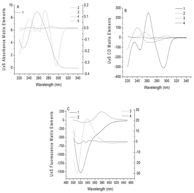
Basis spectra determined using SVD analysis of the data sets in Figure 3 by MATLAB™. The numbers in the plot legends correspond to the rank order of the significant spectroscopic species.

Figure 6.

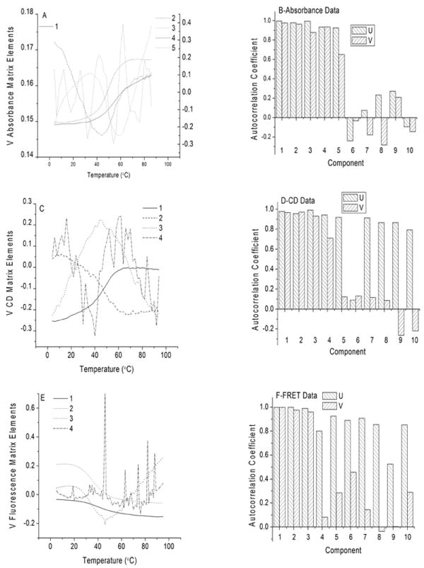
Panels A, C and E show plots of the four or five most significant elements of the V matrices corresponding to the data sets in Figure 3. Panels B, D and F show the autocorrelation coefficients estimated for the first ten significant components of the U and V matrices.

Commentary

Examples of Multi-Dimensional Spectroscopic Melting Data

The use of multi-wavelength spectroscopy to analyze the melting behavior of a 22-residue oligonucleotide model of the human telomeric sequence d[A(GGGTTA)₃] is illustrated below. NMR studies (Wang and Patel, 1993) show that d[A(GGGTTA)₃] (designated here by its PDB code name 143D) forms a quadruplex in NaCl solution that is folded into an antiparallel basket-like structure in which the 5′ and 3′ ends are directly opposed to each other and situated on opposite sides of the basket. Melting profiles for 143D were determined by three spectroscopic methods: UV absorption, CD and fluorescence. The resulting data sets are reproduced in Figure 3.

Figure 3, Panels A and C, show absorption and CD spectra of 143D as a function of temperature. The absorption spectra (Panel A) exhibit clear isosbestic points while the CD spectra (Panel C) lack them. Dual parametric plots for data sets 1A and 1C in which the signal at 295 nm (which specifically monitors quadruplex formation) is plotted against that at 260 nm (which reflects the environment of all bases, including the TTA loop residues) are distinctly non-linear (not shown). Thus, both the UV absorption and CD spectra indicate that more than two species contribute to the spectroscopic changes during thermal unfolding of 143D in NaCl.

Figures 3B and 3D show derivative curves for the changes in absorbance and CD at 295 nm and 260 nm. There are two noticeable features of these plots: (a) for each technique, the apparent Tm value as indicated by the maxima and minima occurs at different temperatures; (b) the apparent Tm values revealed by the two techniques are different.

We next fit each of the derivative curves as described in section 8 above to a two-state model to obtain approximate, preliminary values for Tm and ΔH°. These fits are shown by the solid lines in Figures 3B and 3D and the resulting parameters are in Table 1. It is clear by inspection of the figures that the experimental data points are poorly represented by the two-state model.

Table 1.

Summary of thermodynamic parameters estimated by non-linear least squares fit to Equation 1 describing a two-state equilibrium from the data in Figure 3, panels B, D and F.

Method	Wavelength (nm)	Tm (°C)	ΔH°vH (kcal/mol)	A × 106
Absorbance	295	56.7 ± 0.5	18.7 ± 0.7	10.0 ± 0.3
	260	51.0 ± 0.4	37.4 ± 1.7	-17.6 ± 0.7
CD	295	41.4 ± 0.4	32.0 ± 1.3	-110 ± 4
	260	33.1 ± 1.8	18.4 ± 2.2	800 ± 8
FRET	570	32.1 ± 0.4	46.0 ± 0.4	-50.0 ± 3.1
	520	38.8 ± 0.4	21.0 ± 0.6	210 ± 5

We also carried out a FRET-based melting analysis of a fluorescence derivative of 143D. The fluorescence data shown in Figure 3, Panel E, were obtained using 143D with a 5′6-carboxyfluorescein (6-Fam) tag and a 3′ tetramethylrhodamine (Tamra) tag. The 6-Fam and Tamra moieties serve as a FRET pair in which 6-Fam is the donor and Tamra is the acceptor (Nagatoishi et al., 2007). As a result of the increase in donor-acceptor distance on unfolding, FRET efficiency decreases with increasing temperature, resulting in a temperature-dependent increase in 6-Fam emission at 520 nm and a decrease in Tamra emission at 580 nm when 6-Fam is excited. This behavior is illustrated by the emission spectra in Figure 3E. Note the lack of an isosbestic point in the emission spectra as a function of temperature, suggesting as above that more than two states are present during thermal unfolding. The first derivative plots in Figure 3F show a lack of correspondence in apparent Tm values for donor emission (520 nm, apparent Tm = 41 °C) and acceptor emission (570 nm, apparent Tm = 36 °C). Thus, melting of 6-Fam-143D-Tamra exhibits heterogeneous melting behavior as manifested in the different melting properties of the donor and acceptor FRET tags.

The next sections will show how SVD analysis of the data in Figures 3A, 3C and 3E using MATLAB™ can define the number of spectroscopically distinct species and GlobalWorks™ can carry out a global fit of the data sets to define the thermodynamic parameters that describe the melting process using step-wise models of unfolding. This analysis is described below for each data set in Figure 3.

Figures 4, 5 and 6 illustrate the stepwise analysis of the spectroscopic data of Figure 3 using MATLAB™ to determine the number of significant species, the corresponding basis spectra, and their relative magnitudes during the temperature increase. We first describe determination of the number of significant spectroscopic species using MATLAB™, followed by analysis of each data set by GlobalWorks™.

Figure 4.

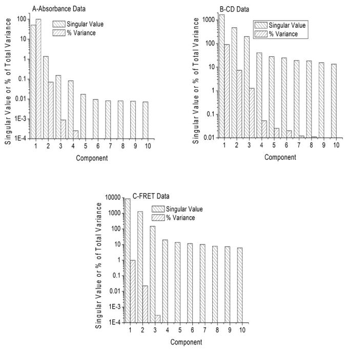
Charts showing the singular values and their relative variance for the first ten significant components of the UV absorbance, CD and FRET data in Figure 3.

1. Determination of number of significant spectroscopic species

It is generally necessary to rely on a combination of factors to determine the number of significant spectroscopic features. These include: (a) comparison of the magnitude of the singular values for each component returned by the SVD analysis; (b) the contribution of each singular value to the total variance of the data set; (c) the resemblance of the basis spectra to recognizable spectral components; (d) examination of the concentration profile of each component as a function of the experimental variable. In the following, we look first at the magnitude of the singular values and their relative variance (plotted as the percentage of the total variance) as an indicator of the importance of each singular value in contributing to the variation in signal with respect to temperature. We then examine the basis spectra as determined in the U×S matrix, followed by the temperature-variation of the species as determined in the V matrix. Calculation of the autocorrelation coefficients for each element the V matrix are also shown to aid in deciding which singular values are significant.

The first step in determining the minimum number of significant species comprising a data set is to examine the singular values and relative fraction of the variance contributed by each. This is illustrated by the bar graphs shown in Figure 4, Panels A, C and E, which illustrate singular values for the first ten components of each data set in Figure 3. The singular values indicate the relative weights of each component of the data matrix. Also shown in Figure 4 is the percent contribution of each component to the total variance of the data set (the Scree plot). Inspection of Figure 4 shows that for the absorbance and CD data sets, the singular values decrease relatively rapidly and reach an approximately constant level (determined by the noise level) after four or five components. For the fluorescence data set (Figure 4C), the singular values become approximately constant after the third value.

There is some ambiguity in determining whether higher order components should be classified as significant. The Scree plot aids in resolving this issue. For example, components 4 and 5 in Figure 4A have nearly identical singular values, but their contribution to the variance differs. Taken together, the singular value and Scree analysis suggests that four components are required to reproduce the absorbance and CD data matrices within the level of noise, while three components may be needed for the FRET data matrix.

2. Characterizing the Basis Spectra of the Significant Species

Plotting the columns of the U×S matrix vs. wavelength results in a representation of the basis spectra which, when combined with the appropriate weights, will reproduce D. Recall that the SVD analysis does not generate the absolute spectra, but rather shows which normalized spectral features can be combined to reproduce the experimental spectrum.

Figure 5 shows the four or five most significant basis spectra for the data sets of Figure 3. Note that the most significant basis spectrum resembles the main features of the experimental spectrum, but may take the shape of a mirror-image spectrum. For example, the most significant spectrum in Figure 5A clearly resembles a typical nucleic acid absorption spectrum, while the second most significant basis spectrum resembles a mirror image of a typical absorbance difference spectrum for the Folded – Unfolded DNA quadruplex in NaCl. The remaining basis spectra are of smaller amplitude and also resemble difference spectra. The third through fifth basis spectra appear as small perturbations of the nucleic acid spectrum. Finally, basis spectrum #5 in Figure 5A is nearly flat, in keeping with its correspondingly smaller singular value and low contribution to the variance. Thus, one may expect the absorbance matrix to consist of four significant species. A similar analysis suggests that four species contribute to the CD matrix and three to the FRET matrix.

3. Characterization of the Temperature Profiles of the Significant Species

The temperature-dependence of the V matrix elements shows the relative weights of each spectral component to the overall absorbance at a particular temperature. This is illustrated in Figure 6. For the UV absorbance data (Panel A), components 1 and 2 resemble melting curves with mid-point temperatures of ~50 °C, the third component has two inflections (~30 °C and ~60 °C), and the fourth component exhibits a U-shaped profile with a minimum at ~40 °C. Component five shows no regular dependence on temperature. Thus, visual inspection of the plot of the V elements vs. temperature suggests at least four spectroscopically species that vary in a regular fashion with temperature.

A quantitative means of examining temperature dependence of the components is to calculate the autocorrelation coefficients of the elements of the V matrix. These calculations are summarized in Figure 4, Panels B, C and D for the absorbance, CD and FRET data sets, respectively. The autocorrelation coefficients of the U matrix elements tend to be rather featureless for the ten most significant species, generally showing high values for at five or more components. However, in keeping with the regular variation in the V matrix elements for the most significant components (Panels A C and E), the autocorrelation coefficients show distinct cutoff values after four components for the absorbance and CD data matrices (Panels B and C), and after three components for the FRET data matrix (Panel D).

4. Fitting the Absorbance-Temperature Data Matrix to a Specific Mechanism

The SVD analysis outlined above provides an indication of the number of species contributing to the signal change over the wavelength and temperature range encompassed by the experimental data. However, the SVD analysis, as discussed above, does not provide the actual spectra of the species or their melting properties. To achieve this goal, one must fit the data set to specific mechanism and optimize the adjustable parameters of the mechanism using a method such as non-linear least squares.

NOTE: In some cases, coupling SVD analysis to the method of evolving factor analysis allows calculation of actual spectra and temperature profiles that are independent of a specific model. The reader is referred to reference (Keesey and Ryan, 1999) for a discussion.

GlobalWorks™ contains algorithms which can fit a data matrix to one of several unfolding mechanisms, including two-, three- and four state processes (e.g. F ↔ U, F ↔ I ↔ U or F ↔ I1 ↔ I2 ↔ U where the I species are intermediates). The basic mechanisms and associated equations have been presented by Greenfield (Greenfield, 2006) and will not be discussed here. To carry out a fit of a data set to a particular mechanism, one must supply starting values for the Tm, ΔH and (if applicable) ΔCp. These values are then optimized by non-linear least squares to fit the complete data set. The optimized parameters are returned along with an estimation of their standard error, the standard deviation of the fit, and graphics showing the calculated spectra of the significant species as well as their concentration profiles as the melt progresses.

Analysis of the data sets in Figure 3 by GlobalWorks™ is summarized in Figure 7. Both UV absorbance and CD, data sets are best described by a four state melting process, while the FRET data set is adequately described by a three-state process. The least-squares optimized parameters Tm and ΔH, along with the standard errors of the fits are summarized in Table 2. For the absorbance and CD data sets, a fit to a two-state or three-state mechanism gave a significantly larger standard deviation of the fit. For the fluorescence data set, the fit to a two-state mechanism resulted in a larger standard deviation. While a fit to a four-state mechanism gave a slightly better standard deviation of the fit, it does not seem justified based on inspection of the basis spectrum of component 4, the autocorrelation coefficient of the V matrix elements and the contribution of component 4 to the variance.

Figure 7.

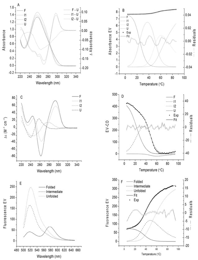
Analysis of absorbance, CD and FRET data matrices of Figure 3 by GlobalWorks™. The absorbance and CD data were fit to a sequential four-state melting process F ↔ I1 ↔ I2 ↔ U where F and U represent the folded and unfolded states, and I1 and I2 are spectroscopic intermediates. EV = eigenvalue, which for the spectra corresponds directly to the measured spectroscopic parameter. For the species distribution plots in Panels B, D and F, EV is related to the relative contribution of each species to the total signal at the particular temperature. Also shown in Panels B, D and F is a comparison of the experimental data (•) and the best fit (solid line) calculated using the least-squares optimized parameters in Table 2. In addition, the distribution of residuals is shown (-o-).

Table 2.

Summary of thermodynamic parameters for melting of 143D in 50 mm NaCl assessed by different techniques derived from analysis of the data in Figure3, Panels A, C and E by GlobalWorks.

Method	Std Dev of Fit	Tm1 (°C)	ΔH1 (kcal/mol)	Tm2 (°C)	ΔH2 (kcal/mol)	Tm3 (°C)	ΔH3 (kcal/mol)
Absorbance	0.0006	24.5 ± 1.6	33.4 ± 0.2	51.8 ± 0.6	35.4 ± 1.3	70.1 ± 1.0	16.5 ± 0.4
CD	0.566	23.0 ± 0.7	21.7 ± 0.7	49.5 ± 0.5	34.5 ± 0.6	71.6 ± 1.6	17 ± 3
FRET	0.639			38.0 ± 0.4	24.6 ± 1.9	58.7 ± 0.2	14.4 ± 0.6

Comments

The spectral shapes identified for the intermediate species could be used to infer some structural information regarding these species. For example, spectral features in the 295 nm region most certainly reflect formation of the G-quartets, while structural features in the 260-270 nm region may include effects on other bases. Moreover, the formation of a structure with an intermediate FRET efficiency may reflect one in which the donor and acceptor tags are separated more than they are in the fully folded structure but less than in the unfolded ensemble. In addition, it probably goes without saying that just because a particular data set fits well to a particular mechanism does not prove that the particular mechanism applies. Obviously other mechanisms not tested conceivably could fit the data as well or better. However, the multi-wavelength, multi-method approach to thermal unfolding studies clearly provides a basis for further analysis to ascertain the structures of the intermediate states.

References

- Bishop GR, Chaires JB. Measuring Circular Dichroism. Curr Protocol Nucleic Acid Chem. 2002:7.11.11–17.11.18. doi: 10.1002/0471142700.nc0711s11. [DOI] [PubMed] [Google Scholar]
- Cattell RB. The Scree Test For The Number Of Factors<sup>1</sup>. Multivariate Behavioral Research. 1966;1:245–276. doi: 10.1207/s15327906mbr0102_10. [DOI] [PubMed] [Google Scholar]
- DeSa RJ, Matheson IB. A practical approach to interpretation of singular value decomposition results. Methods Enzymol. 2004;384:1–8. doi: 10.1016/S0076-6879(04)84001-1. [DOI] [PubMed] [Google Scholar]
- Gralla J, Crothers DM. Free energy of imperfect nucleic acid helices. II. Small hairpin loops. J Mol Biol. 1973;73:497–511. doi: 10.1016/0022-2836(73)90096-x. [DOI] [PubMed] [Google Scholar]
- Greenfield NJ. Using circular dichroism collected as a function of temperature to determine the thermodynamics of protein unfolding and binding interactions. Nat Protoc. 2006;1:2527–2535. doi: 10.1038/nprot.2006.204. [DOI] [PMC free article] [PubMed] [Google Scholar]
- Haq I, Chowdhry BZ, Chaires JB. Singular value decomposition of 3-D DNA melting curves reveals complexity in the melting process. Eur Biophys J. 1997;26:419–426. doi: 10.1007/s002490050096. [DOI] [PubMed] [Google Scholar]
- Hendler RW, Shrager RI. Deconvolutions based on singular value decomposition and the pseudoinverse: a guide for beginners. J Biochem Biophys Methods. 1994;28:1–33. doi: 10.1016/0165-022x(94)90061-2. [DOI] [PubMed] [Google Scholar]
- Henry RW, Hofrichter J. Singular value decomposition: application to analysis of experimental data. In: Brand L, Johnson ML, editors. Methods in Enzymology. Vol. 210. Academic Press; New York: 1992. pp. 129–191. [Google Scholar]
- John DM, Weeks KM. van’t Hoff enthalpies without baselines. Protein Sci. 2000;9:1416–1419. doi: 10.1110/ps.9.7.1416. [DOI] [PMC free article] [PubMed] [Google Scholar]
- Keesey RL, Ryan MD. Use of evolutionary factor analysis in the spectroelectrochemistry of Escherichia coli sulfite reductase hemoprotein and a Mo/Fe/S cluster. Anal Chem. 1999;71:1744–1752. doi: 10.1021/ac981079h. [DOI] [PubMed] [Google Scholar]
- Lumry R, Biltonen R. Validity of the “two-state” hypothesis for conformational transitions of proteins. Biopolymers. 1966;4:917–944. doi: 10.1002/bip.1966.360040808. [DOI] [PubMed] [Google Scholar]
- Mergny J-L, Lacroix L. UV Melting of G-Quadruplexes. Curr Protocol Nucleic Acid Chem. 2009;37:17.11.11–17.11.15. doi: 10.1002/0471142700.nc1701s37. [DOI] [PubMed] [Google Scholar]
- Nagatoishi S, Nojima T, Galezowska E, Gluszynska A, Juskowiak B, Takenaka S. Fluorescence energy transfer probes based on the guanine quadruplex formation for the fluorometric detection of potassium ion. Anal Chim Acta. 2007;581:125–131. doi: 10.1016/j.aca.2006.08.010. [DOI] [PubMed] [Google Scholar]
- Wallimann P, Kennedy RJ, Miller JS, Shalongo W, Kemp DS. Dual wavelength parametric test of two-state models for circular dichroism spectra of helical polypeptides: anomalous dichroic properties of alanine-rich peptides. J Am Chem Soc. 2003;125:1203–1220. doi: 10.1021/ja0275360. [DOI] [PubMed] [Google Scholar]
- Wang Y, Patel DJ. Solution structure of the human telomeric repeat d[AG3(T2AG3)3] G-tetraplex. Structure. 1993;1:263–282. doi: 10.1016/0969-2126(93)90015-9. [DOI] [PubMed] [Google Scholar]