Neural correlates of reliability-based cue weighting during multisensory integration

Abstract

Integration of multiple sensory cues is essential for precise and accurate perception and behavioral performance, yet the reliability of sensory signals can vary across modalities and viewing conditions. Human observers typically employ the optimal strategy of weighting each cue in proportion to its reliability, but the neural basis of this computation remains poorly understood. We trained monkeys to perform a heading discrimination task from visual and vestibular cues, varying cue reliability at random. Monkeys appropriately placed greater weight on the more reliable cue, and population decoding of neural responses in area MSTd nicely predicted behavioral cue weighting, including modest deviations from optimality. We further show that the mathematical combination of visual and vestibular inputs by single neurons is generally consistent with recent theories of optimal probabilistic computation in neural circuits. These results provide direct evidence for a neural mechanism mediating a simple and widespread form of statistical inference.

INTRODUCTION

The information received through our senses is inherently probabilistic, and a key challenge for the brain is to construct an accurate representation of the world despite this uncertainty. This problem is particularly relevant when considering the integration of multiple sensory cues, since the reliability associated with each cue can vary rapidly and unpredictably. Numerous psychophysical studies^1–8 have shown that human observers combine cues by weighting them in proportion to their reliability, consistent with statistically optimal (e.g., Bayesian or maximum-likelihood) schemes. This solution is optimal because it generates unbiased perceptual estimates with the lowest possible variance^{9, 10}, leading to an improvement in psychophysical performance beyond what can be achieved with either cue alone, or with any ad hoc weighting scheme.

The neural basis of optimal cue integration is not well understood, in part because of a lack of neurophysiological measurements in behaving animals. Recently, we developed a paradigm in which macaque monkeys discriminate their direction of translational self-motion (heading) from visual and/or vestibular cues¹¹. We found that monkeys can integrate these cues to improve psychophysical performance, in accordance with one key prediction of optimal cue integration models. We also identified a population of multimodal neurons in the dorsal medial superior temporal area (MSTd) that likely form part of the neuronal substrate for this integration. MSTd neurons with congruent visual and vestibular heading tuning showed increased sensitivity during presentation of multimodal stimuli, analogous to the perceptual improvement¹¹. Our previous work also demonstrated significant trial-by-trial correlations between neuronal activity and monkeys’ perceptual decisions (‘choice probabilities’), suggesting a functional link between MSTd activity and performance in this task^{11, 12}.

This earlier study¹¹ revealed neural correlates of increased sensitivity during cue integration (with cue reliabilities fixed), but did not explore how multisensory neurons could account for the second key prediction of optimal cue integration: weighting cues according to their relative reliabilities. Behaviorally, reliability-based cue weighting can be measured by introducing a small conflict between cues and asking to what extent subjects’ perceptual choices favor the more reliable cue^1–6. Using this approach, we showed that monkeys, like humans, can reweight cues (that is, adjust weights from trial to trial) according to their reliability in a near-optimal fashion¹³. The present study goes on to address two fundamental questions regarding the neural basis of reliability-based cue weighting. First, can the activity of a population of multisensory neurons predict behavioral reweighting of cues as reliability varies? We show that a simple decoding of MSTd neuronal activity, recorded during a cue-conflict task, can account remarkably well for behavioral reweighting, including some modest deviations from optimality and individual differences between subjects. Second, what mathematical operations need to take place in single neurons, such that a simple population code can account for behavioral cue reweighting? We report that neurons combined their inputs linearly with weights dependent on cue reliability, in a way broadly consistent with the theory of probabilistic population codes¹⁴. These findings establish, for the first time, a link between empirical observations of multisensory integration in single neurons and optimal cue integration at the level of behavior.

RESULTS

Theoretical predictions and behavioral performance

We begin by outlining the key predictions of optimal cue integration theory, and how we tested these predictions in behaving monkeys. Following the standard (linear) ideal-observer model of cue integration¹⁵, we postulate an internal heading signal S_comb that is a weighted sum of vestibular and visual heading signals S_ves and S_vis (where w_vis = 1 − w_ves):

$$S_{\mathit{comb}}=w_{\mathit{ves}}{S}_{\mathit{ves}}+w_{\mathit{vis}}{S}_{\mathit{vis}}$$ (1)

If each S is considered a Gaussian random variable with mean μ and variance σ², the optimal estimate of μ_comb (minimizing its variance while remaining unbiased) is achieved by setting the weights in Eq. 1 proportional to the reliability (i.e., inverse variance) of S_ves and S_vis^{6, 10}:

$$w_{\mathit{ves}-\mathit{opt}}=\frac{1/{\sigma }_{\mathit{ves}}^2}{1/{\sigma }_{\mathit{ves}}^2+1/{\sigma }_{\mathit{vis}}^2};w_{\mathit{vis}-\mathit{opt}}=\frac{1/{\sigma }_{\mathit{vis}}^2}{1/{\sigma }_{\mathit{ves}}^2+1/{\sigma }_{\mathit{vis}}^2}$$ (2)

The combined reliability is equal to the sum of the individual cue reliabilities:

$$\frac{1}{{\sigma }_{\mathit{comb}}^2}=\frac{1}{{\sigma }_{\mathit{ves}}^2}+\frac{1}{{\sigma }_{\mathit{vis}}^2}$$

Or, solving for σ_comb:

$${\sigma }_{\mathit{comb}-\mathit{opt}}=\sqrt{\frac{{\sigma }_{\mathit{ves}}^2{\sigma }_{\mathit{vis}}^2}{{\sigma }_{\mathit{ves}}^2+{\sigma }_{\mathit{vis}}^2}}$$ (3)

Eq. 3 formalizes the intuition that multisensory estimates should be more precise than single-cue estimates (i.e., resulting in improved discrimination performance), with the maximum effect being a reduction in σ by a factor of the square root of 2 when single-cue reliabilities are matched. Note that the predictions specified by Eqs. 2 and 3 are the same if optimality is defined in the Bayesian (maximum a posteriori) sense, assuming Gaussian likelihoods and a uniform prior^{3, 4, 6, 15, 16}.

To test these predictions, we trained two monkeys to report their heading relative to a fixed, internal reference of straight ahead (a one-interval, 2-alternative forced-choice task). Heading stimuli could be presented in one of three modalities: ‘vestibular’ (inertial motion delivered by a motion platform), ‘visual’ (optic flow simulating observer movement through a random-dot cloud), or ‘combined’ (simultaneous inertial motion and optic flow; see Methods and refs. ^{11–13, 17}). On combined trials, we pseudorandomly varied the conflict angle (Δ) between the headings specified by visual and vestibular cues (Δ = −4°, 0°, or 4°; Fig. 1a). By convention, Δ = +4° indicates that the visual cue was displaced 2° to the right of the assigned heading value for that trial, while the vestibular cue was 2° to the left (and vice versa for Δ = −4°). To manipulate cue reliability, we also varied the percentage of coherently moving dots in the visual display (motion coherence; 16% or 60%). We chose these values for motion coherence to set the reliability of the visual cue (as measured by behavioral performance) above and below that of the vestibular cue, for which reliability was held constant.

Figure 1.

Cue-conflict configuration and example behavioral session. (a) Monkeys were presented with visual (optic flow) and/or vestibular (inertial motion) heading stimuli in the horizontal plane. The heading (θ) was varied in fine steps around straight ahead, and the task was to indicate rightward or leftward heading with a saccade after each trial. On a subset of visual-vestibular (‘combined’) trials, the headings specified by each cue were separated by a conflict angle (Δ) of ±4°, where positive Δ indicates visual to the right of vestibular, and vice versa for negative Δ. (b) Psychometric functions for an example session, showing the proportion of rightward choices as a function of heading for the single-cue conditions. Psychophysical thresholds were taken as the standard deviation (σ) of the best-fitting cumulative Gaussian function (smooth curves) for each modality. Single-cue thresholds were used to predict (via Eq. 2) the weights that an optimal observer should assign to each cue during combined trials. (c) Psychometric functions for the combined modality at low (16%) coherence, plotted separately for each value of Δ. The shifts of the points of subjective equality (PSEs) during cue-conflict were used to compute ‘observed’ vestibular weights (Eq. 4). (d) Same as c, but for the high-(60%) coherence combined trials.

Behavioral data (see also ref. ¹³) indicate that monkeys reweight visual and vestibular heading cues on a trial-by-trial basis in proportion to their reliability, as illustrated for an example session in Fig. 1b–d. Psychometric data (proportion rightward choices as a function of heading) were fit with cumulative Gaussian functions, yielding two parameters: the point of subjective equality (PSE; mean of the fitted cumulative Gaussian function) and the threshold (defined as its standard deviation, σ). Similar to previous studies^{1–6, 8}, thresholds from single-cue conditions (Fig. 1b) were used to estimate the relative reliability of the two cues, which specifies the weights that an optimal observer should apply to each cue (Eq. 2). These ‘optimal’ weights were computed from Eq. 2 by pairing the vestibular threshold (σ = 3.3° in this example; Fig. 1b) with each of the two visual thresholds (16% coh., σ = 5.1°; 60% coh., σ = 1.1°). Optimal vestibular weights for this session were 0.70 and 0.10 for low and high coherence, respectively (recall that w_vis = 1 − w_ves; we report only vestibular weights for simplicity).

On cue-conflict trials (Fig. 1c,d), the monkey’s choices were biased toward the more reliable cue, as indicated by lateral shifts of the psychometric functions for Δ = ±4°, relative to Δ = 0°. At 16% coherence (Fig. 1c), when the vestibular cue was more reliable, the monkey made more rightward choices for a given heading when the vestibular cue was displaced to the right (Δ = −4°, blue curve), and more leftward choices when the vestibular cue was to the left (Δ = +4°, green curve). This pattern was reversed when the visual cue was more reliable (60% coherence; Fig. 1d). We used the shifts in the PSEs to compute ‘observed’ vestibular weights, according to a formula derived from the same framework (Eq. 1) as the optimal weights (see Methods for derivation):

$$w_{\mathit{ves}-\mathit{obs}}=\frac{{\mathit{PSE}}_{\mathit{comb}}-{\mathit{PSE}}_{\mathit{comb},\mathrm{\Delta }=0}+\frac{\mathrm{\Delta }}{2}}{\mathrm{\Delta }}$$ (4)

For the dataset in Fig. 1c,d, the observed vestibular weights were 0.72 and 0.08 for 16% and 60% coherence, respectively.

Vestibular weights for two monkeys are summarized in Fig. 2a,b. Both monkeys showed robust changes in observed weights as a function of coherence (session-wise paired t-tests: monkey Y, N = 40 sessions, p < 10⁻²⁸; monkey W, N = 26, p < 10⁻¹³). Observed weights were reasonably close to the optimal predictions, especially for monkey Y (Fig. 2a). However, there were significant deviations from optimality in both animals (as reported previously for a larger sample of monkey and human subjects¹³), with the most consistent effect being an over-weighting of the vestibular cue at low coherence (paired t-tests, observed > optimal at 16% coh.: monkey W, p < 10⁻⁸; monkey Y, p < 10⁻⁶). Monkey W also over-weighted the vestibular cue at high coherence (60%: p < 10⁻⁵), but the opposite trend was observed for monkey Y (observed < optimal at 60%, p = 0.003). These types of deviations from optimality – apparent over- or under-weighting of a particular sensory cue – are not unprecedented in the human psychophysics literature^{5, 18, 19}, and present an opportunity to look for neural signatures of the particular deviations we observed.

Figure 2.

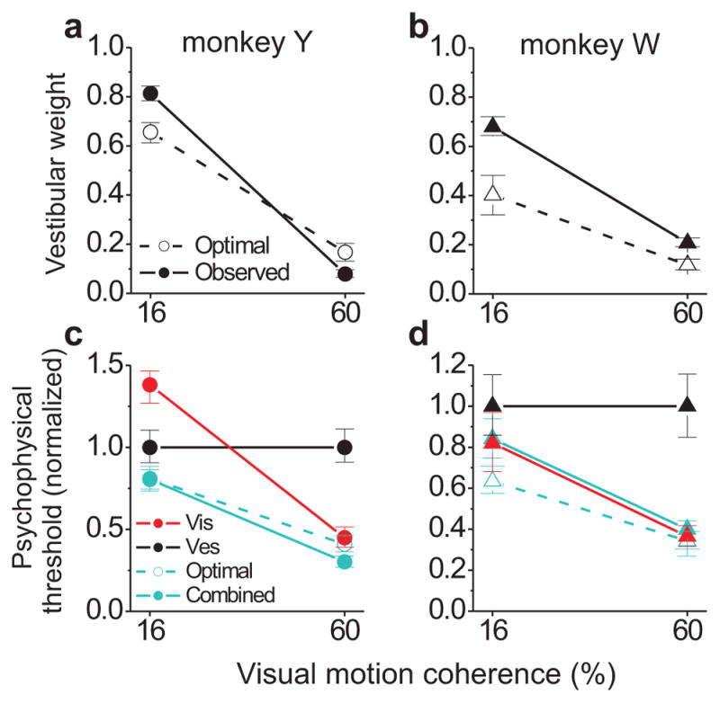
Average behavioral performance. (a,b) Optimal (Eq. 2, open symbols and dashed line) and observed (Eq. 4, filled symbols and solid line) vestibular weights as a function of visual motion coherence (cue reliability), shown separately for the two monkeys (a, monkey Y, N = 40 sessions; b, monkey W, N = 26). (c,d) Optimal (Eq. 3) and observed (estimated from the psychometric fits) psychophysical thresholds, normalized separately by each monkey’s vestibular threshold. Error bars in a–d represent 95% confidence intervals computed with a bootstrap procedure.

The corresponding psychophysical thresholds for the two monkeys are shown in Fig. 2c,d. Note that, unlike our previous work¹¹, the present study was not designed to reveal optimal improvements in psychophysical thresholds under cue combination (Eq. 3), as coherence was never chosen to equate the single-cue thresholds here. Nevertheless, we generally observed near-optimal sensitivity in the combined modality (Fig. 2c,d). The most notable deviation was the case of 16% coherence for monkey W, which is also the condition of greatest vestibular over-weighting (Fig. 2b).

Single-neuron correlates of cue reweighting

To explore the neural basis of these behavioral effects, we recorded single-unit activity from cortical area MSTd, an extrastriate region that receives both visual and vestibular signals related to self-motion^{12, 17, 20, 21}. Our primary strategy was to decode a population of MSTd responses to predict behavioral choices under each set of experimental conditions, thereby constructing simulated psychometric functions from decoded neural responses. We then repeated the analyses of the previous section to test whether MSTd activity can account for cue integration behavior in this task. These analyses were performed on a sample of 108 neurons (60 from monkey Y, 48 from monkey W) that had significant tuning for at least one stimulus modality over a small range of headings near straight ahead (see Methods for detailed inclusion criteria).

Before describing the decoding results, we first illustrate the basic pattern of responses seen in individual neurons. Tuning curves (firing rate as a function of heading) for an example neuron are plotted in Fig. 3a–c. As for most MSTd neurons^{11, 12}, the tuning is approximately linear over the small range of headings tested in the discrimination task (±10°). This neuron showed significant tuning and a preference for leftward headings in all conditions/modalities. Note that the tuning curves from cue-conflict trials (Fig. 3b,c) shifted up or down depending on both the direction of the conflict (the sign of Δ) and the relative cue reliability (motion coherence). For most headings, the example neuron responded to the cue-conflict with an increase or decrease in firing rate depending on which cue was more ‘reliable’ in terms of neuronal sensitivity. Take for instance the combined tuning at 60% coherence when Δ = −4° (visual heading to the left of vestibular; Fig. 3c). Because the cell preferred leftward headings, the dominance of the more reliable visual cue resulted in a greater firing rate relative to the orange Δ = 0° curve (and vice versa for Δ = +4°). The direction of the shifts was largely reversed at 16% coherence (Fig. 3b), for which the vestibular cue was more reliable.

Figure 3.

Example MSTd neuron showing a correlate of trial-by-trial cue reweighting. Mean firing rate (spikes/s) ± s.e.m. is plotted as a function of heading for the single-cue trials (a), and combined trials at low (b) and high (c) coherence. The shift in combined tuning curves with cue conflict, in opposite directions for the two levels of reliability, forms the basis for the reweighting effects in the population decoding analysis depicted in Figs. 4 and 6 (see Supplementary Figs. S1 and S2 for single-cell neurometric analyses).

These effects of cue-conflict and coherence on tuning curves suggest that MSTd neurons may be performing a weighted summation of inputs, as discussed further below. We now consider whether these relatively simple changes in firing rates can account for the perceptual effects of cue reliability. Because perception arises from the concurrent activity of many neurons, we focus on making behavioral predictions from population activity using a decoding approach. We also performed cell-by-cell neurometric analyses (see Supplementary Material, online, for methods), which gave similar results (see Supplementary Figs. S1 and S2).

Likelihood-based decoding of MSTd neuronal populations

We used a well-established method of maximum-likelihood decoding^22–24 to convert MSTd population responses into perceptual choices made by an ideal observer performing the heading discrimination task. Our approach was to simulate population activity on individual trials by pooling responses from our sample of MSTd neurons, a strategy made possible by having a fixed set of stimuli and conditions across recording sessions. On each simulated trial, the decoder estimated the most likely heading based on the population response. Responses (r) were generated by taking random draws of single-trial firing rates from each recorded neuron under the particular set of conditions (stimulus modality, heading (θ), and conflict angle (Δ)) being simulated on that trial. We then computed the full likelihood function P(r|θ) using an expression (Eq. 14, Methods) that assumes independent Poisson variability (see Supplementary Material for details; relaxing the assumptions of independence and Poisson noise did not substantially affect the results). Assuming a flat prior, we normalized the likelihood to obtain the posterior distribution, P(θ|r), then computed the area under the posterior favoring leftward vs. rightward headings. When the integrated posterior for rightward headings exceeded that for leftward headings, the ideal observer registered a ‘rightward’ choice, and vice-versa.

Importantly, cue-conflict trials were decoded with respect to the non-conflict (Δ = 0°) tuning curves (e.g., see Fig. 3b,c). The implicit assumption here is that the decoder, or downstream area reading out MSTd activity, does not alter how it interprets the population response based on the (unpredictable) presence or absence of a cue-conflict. Given that animals typically experience self-motion without a consistent conflict between visual and vestibular cues, it is reasonable to assume that the brain interprets neuronal responses as though there was no cue-conflict. This assumption allows the shift in tuning curves due to the cue-conflict (Fig. 3b,c) to manifest as a shift in the likelihoods, and hence the PSE of the simulated psychometric functions, as described below.

Examples of likelihood functions derived from our full sample of MSTd neurons (N = 108) in the single-cue conditions are shown in Fig. 4a,b. Results from 4 representative trials are overlaid for a constant simulated heading of 1.2°. Note that the vestibular (Fig. 4a) and low-coherence visual (Fig. 4b) likelihoods are more variable in their position on the heading axis compared to the high-coherence visual condition (Fig. 4b). This differential variability is reflected in the slopes of the simulated psychometric functions produced by the decoder (Fig. 4c), which yielded thresholds of 0.41°, 0.38°, and 0.27°, respectively. From Eq. 2, these threshold values gave optimal vestibular weights of 0.46 and 0.30 for low and high coherence, respectively.

Figure 4.

Likelihood-based decoding approach used to simulate behavioral performance based on MSTd activity. (a,b) Example likelihood functions (P(r|θ)) for the single-cue modalities. Four individual trials of the same heading (θ = 1.2°, green arrow) are superimposed for each condition. Likelihoods were computed from Eq. 14 using simulated population responses (r) comprised of random draws of single-neuron activity. (c) Simulated psychometric functions for a decoded population that included all 108 MSTd neurons in our sample. (d,e) Combined modality likelihood functions for θ = 1.2° (green arrow and dashed line) and Δ = +4°, for low (cyan) and high (blue) coherence. Black and red inverted triangles indicate the headings specified by vestibular and visual cues, respectively, in this stimulus configuration. (f) Psychometric functions for the simulated combined modality, showing the shift in the PSE due to coherence (i.e., reweighting).

Fig. 4d,e shows combined modality likelihoods for the same simulated heading of 1.2°, when a positive cue-conflict (Δ = +4°) was introduced. In this stimulus condition, the visual heading is +3.2° and the vestibular heading is −0.8° (red and black triangles, respectively). At 16% coherence (Fig. 4d), the likelihood functions tended to peak closer to the vestibular heading, whereas at 60% coherence (Fig. 4e) they peaked closer to the visual heading. This generated more leftward choices at low coherence and more rightward choices at high coherence, and thus a shift of the combined psychometric function in opposite directions relative to zero (Fig. 4f). The observed weights corresponding to these PSE shifts were 0.80 and 0.14 for low and high coherence, respectively (p ≪ 0.05, bootstrap). Thus, the population decoding approach reproduced the robust cue reweighting effect observed in the behavior (Fig. 2a,b). It is important to emphasize that, because coherence was varied randomly from trial to trial, this neural correlate of cue reweighting in MSTd must occur fairly rapidly (i.e., on the timescale of each 2-second trial).

Decoding summary and the effect of tuning congruency

Previously¹¹ we reported that the relative tuning for visual and vestibular heading cues in MSTd varies along a continuum from congruent to opposite, where congruency in the present context refers to the similarity of tuning slopes for the two single-cue modalities. We quantified this property for each neuron using a congruency index (CI), defined as the product of Pearson correlation coefficients comparing firing rate vs. heading for the two modalities¹¹ (Fig. 5a). Positive CI values indicate visual and vestibular tuning curves with consistent slopes, negative values indicate opposite tuning slopes, and values near 0 occur when the tuning curve for either modality is flat or even-symmetric. Our previous study¹¹ used a statistical criterion on the CI to classify neurons as ‘congruent’ or ‘opposite’; however, we found this to be too restrictive for the present dataset, as it did not permit sufficient sample sizes to be analyzed for each animal and congruency class. Thus, here we defined congruent and opposite cells by an arbitrary criterion of CI > 0.4 (N = 46/108, 43%) or CI < −0.4 (N = 23/108, 21%), respectively. We obtained similar results for different CI criteria (±0.5, ±0.2, or simply CI > 0 vs. < 0).

Figure 5.

Visual-vestibular congruency and average MSTd tuning curves. (a) Histogram of congruency index (CI) values for monkey Y (top), monkey W (middle), and both animals together (bottom). Positive congruency index values indicate consistent tuning slope across visual (60% coh.) and vestibular single-cue conditions, while negative values indicate opposite tuning slopes. Filled bars indicate CI values whose constituent correlation coefficients were both statistically significant¹¹; however, here we defined ‘congruent’ and ‘opposite’ cells by an arbitrary criterion of CI > 0.4 and CI < −0.4, respectively. (b,c) Population average of MSTd tuning curves for the 5 stimulus – conditions vestibular (black), low coherence visual (magenta, dashed), high coherence visual (red), low coherence combined (cyan, dashed), and high coherence combined (blue) – separated into congruent (b) and opposite (c) classes. Prior to averaging, some neurons’ tuning preferences were mirrored such that all cells preferred rightward heading in the high coherence visual modality.

Congruency is an important attribute for decoding MSTd responses because only congruent cells show increased heading sensitivity during cue combination that parallels behavior¹¹. This can be seen in our dataset by examining the relative slopes of average tuning curves for each stimulus modality (Fig. 5b; aligned so that all cells prefer rightward in the visual modality). The combined tuning curve of congruent cells at 16% coherence is steeper than either of the single-cue tuning curves, and likewise at 60% coherence, resulting in improved neuronal sensitivity (see also Supplementary Fig. S3, online). In contrast, opposite cells are generally less sensitive to heading under combined stimulation because the visual and vestibular signals counteract each other and the tuning becomes flatter (Fig. 5c). Thus, we examined how decoding subpopulations of congruent and opposite cells compares to decoding all neurons.

Decoding all cells without regard to congruency (N = 108), as mentioned above, yielded a strong reweighting effect (Fig. 6a) but did not reproduce the improvement in psychophysical threshold that is characteristic of behavioral cue integration (Fig. 6b). This outcome is not surprising given the contribution of opposite cells (Fig. 6c,d), for which combined thresholds were substantially worse than thresholds for the best single cue. In contrast, decoding only congruent cells yielded both robust cue reweighting (Fig. 6e) and a significant reduction in threshold (Fig. 6f), matching the behavioral results (Fig. 6g,h) quite well. Interestingly, this subpopulation of congruent neurons also reproduced the overweighting of the vestibular cue at low coherence and the slight under-weighting at high coherence (Fig. 6e,g). These findings support the hypothesis that congruent cells in MSTd are selectively read out to support cue integration behavior¹¹, and suggest that the neural representation of heading in MSTd may contribute to deviations from optimality in this task.

Figure 6.

Population decoding results and comparison with monkey behavior. Weights (left column, same format as Fig. 2a,b; from Eqs. 2 and 4) and thresholds (right column, same format as Fig. 2c,d; from Eq. 3 and psychometric fits to real or simulated choice data) quantifying the performance of an optimal observer reading out MSTd population activity. Thresholds were normalized by the value of the vestibular threshold, and the optimal prediction for the combined modality (cyan dashed lines and open symbols) was computed with Eq. 3. The population of neurons included in the decoder was varied in order to examine the readout of all cells (a,b), opposite cells only (c,d), or congruent cells only (e,f). Monkey behavioral performance (pooled across the two animals) is summarized in g,h. Error bars indicate 95% CIs.

We also compared behavior with decoder performance for each animal separately. Despite the small samples of congruent cells (N = 32 for monkey Y, 14 for monkey W), the decoder captured a number of aspects of the individual differences between animals in weights and thresholds (Supplementary Fig. S4, online). This suggests that individual differences in cue integration behavior may at least partly reflect differences in the neural representation of heading in MSTd.

Multisensory neural combination rule: optimal vs. observed

Thus far we have shown that decoded MSTd responses can account for behavior, but we have not considered the computations taking place at the level of single neurons. Returning to Eq. 1, consider that instead of dealing with abstract signals S_ves and S_vis, the brain must combine signals in the form of neural firing rates. We now describe, at a mechanistic level, how multisensory neurons should combine their inputs in order to achieve optimal cue integration, and then we test whether MSTd neurons indeed follow these predictions. Our previous work²⁵ established that a linear combination rule is sufficient to describe the combined firing rates (tuning curves) of most MSTd neurons:

$$f_{\mathit{comb}}(\theta ,c)=A_{\mathit{ves}}(c)f_{\mathit{ves}}(\theta )+A_{\mathit{vis}}(c)f_{\mathit{vis}}(\theta ,c)$$ (5)

where f_ves, f_vis and f_comb are the tuning curves of a particular MSTd neuron for the vestibular, visual and combined modalities, θ represents heading, c denotes coherence, and A_ves and A_vis are the neural weights (we use the term neural weights to distinguish them from the perceptual weights of Eqs. 1 and 2).

The key issue is to understand the relationship between the perceptual weights (w_ves and w_vis in Eq. 1) and the neural weights (A_ves and A_vis in Eq. 5). One might expect that neural and perceptual weights should exhibit the same dependence on cue reliability (coherence); i.e., that the neural vestibular weights, A_ves, should decrease with coherence as do the perceptual weights (Fig. 2a,b). Importantly, however, this needs not be the case: the relationship between perceptual and neural weights depends on the statistics of the neuronal spike counts, and on how the tuning curves are modulated by coherence. If neurons fire with Poisson statistics and tuning curves are multiplicatively scaled by coherence, then the optimal neural weights will be equal to 1 and independent of coherence¹⁴, whereas the perceptual weights still clearly depend on coherence. For other dependencies of tuning curves on cue reliability, neural and perceptual weights may share a similar dependence on coherence, but this remains to be demonstrated.

It is therefore critical that we derive the predicted optimal neural weights for the MSTd neurons that we have recorded. In our data, coherence does not have a simple multiplicative effect on tuning curves. Instead, as expected from the properties of MT²⁶ and MST²⁷ neurons when presented with conventional random-dot stimuli, the effect of coherence in MSTd is better described as a scaling plus a baseline that decreases with coherence:

$$f_{\mathit{vis}}=\alpha {cf}^{\ast }+\beta (1-c)$$ (6)

(here, f^* is a generic linear tuning function, α and β are constants and c denotes coherence). We did not quantify this effect here, but it can be visualized in Fig. 3a and Fig. 5b,c, (see also Figure S3 in ref. ²⁵ for an illustration with the full heading tuning curve).

Using Eq. 5 and a few well-justified assumptions, we can derive the optimal neural weights (see Supplementary Material for details). This derivation yields a simple expression for the optimal ratio of neural weights, ρ_opt, where ρ_opt = A_ves-opt / A_vis-opt:

$${\rho }_{\mathit{opt}}(c)=\frac{{f^{\prime }}_{\mathit{ves}}(0)f_{\mathit{vis}}(0,c)}{f_{\mathit{ves}}(0){f^{\prime }}_{\mathit{vis}}(0,c)}$$ (7)

In this equation, f′_ves and f′_vis denote the derivatives of the tuning curves with respect to θ, and all terms are evaluated at the reference heading (θ = 0°). Substituting Eq. 6 into Eq. 7, we obtain:

$${\rho }_{\mathit{opt}}=\frac{{f^{\prime }}_{\mathit{ves}}}{f_{\mathit{ves}}}(\frac{f^{\ast }}{{f^{\ast }}^{\prime }}-\frac{\beta }{{{\alpha f}^{\ast }}^{\prime }}+\frac{\beta }{{{\alpha f}^{\ast }}^{\prime }c})$$ (8)

which predicts that the optimal weight ratio is inversely proportional to coherence.

Now that we have an expression for the optimal neural weight ratio (Eq. 7), we can test whether the neural weights measured in MSTd are consistent with optimal predictions. We measured neural weights for MSTd cells in a previous study²⁵, but in that study the monkeys were passively fixating rather than performing a psychophysical task. The present work is also the first to measure neural weights with multiple interleaved levels of cue reliability, and the first to test whether these weights are optimal (as defined by Eq. 7). We fit Eq. 5 to responses of all neurons (N = 108), separately for the two coherence levels, and plotted the distribution of R² values for the fits in Fig. 7a,b. Despite having only 2 free parameters (A_ves and A_vis) for each coherence, the model explained the data reasonably well for most neurons (Fig. 7a,b; low coherence: 88/108 cells (81%) with significant correlation between responses and model fits, p < 0.05; high coherence: 94/108 (87%)). Some poor fits are expected because several neurons had vestibular or low-coherence visual tuning curves that were essentially flat. Consistent with previous findings²⁵, the neural weights changed as a function of coherence, with A_ves decreasing and A_vis increasing as coherence increased (Fig. 7c,d; paired t-test comparing 16% vs. 60% coherence, p < 10⁻⁷ for both A_ves and A_vis). For the majority of neurons (51% of all cells, 68% of congruent cells), a version of the model in which weights were allowed to vary with coherence (‘independent-weights’ model) provided significantly better fits (sequential F-test, p < 0.05) than a model with a single set of weights for both coherences (‘yoked-weights’ model; see Methods and ref. ²⁵). Because coherence was randomized from trial to trial, these changes in neural weights must have occurred on a rapid time scale and are therefore unlikely to reflect changes in synaptic weights (see Discussion and ref. ²⁸). Indeed, examining the time course of neural weights across the 2-s trial duration (Supplementary Fig. S5, online) revealed that the effect was established shortly after response onset and persisted through most of the stimulus duration.

Figure 7.

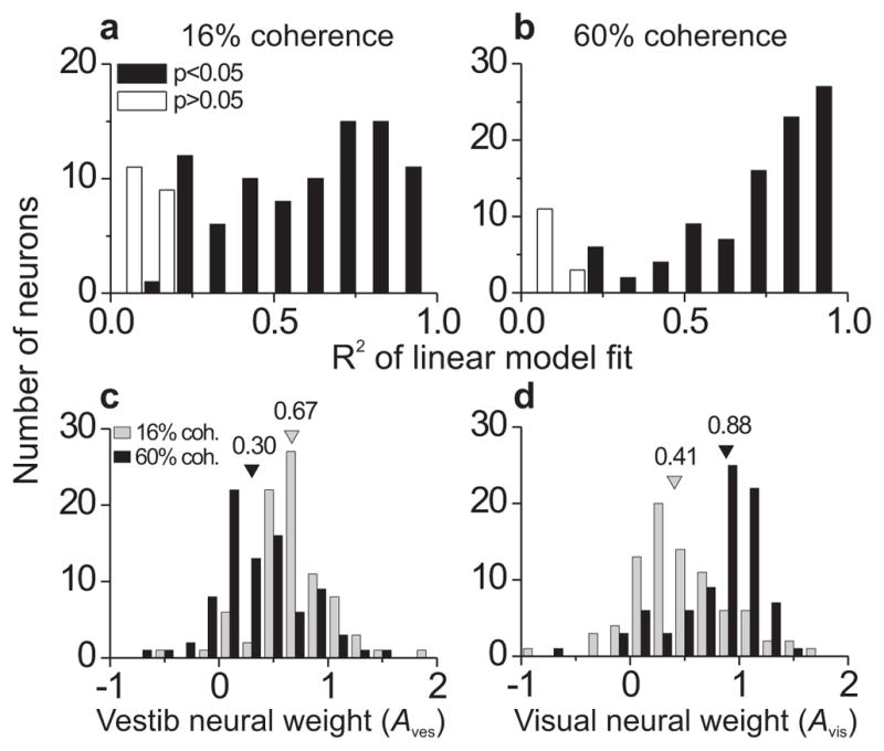
Goodness-of-fit of linear weighted sum model and distribution of vestibular and visual neural weights. Combined responses during the discrimination task (N = 108) were modeled as a weighted sum of visual and vestibular responses, separately for each coherence level. (a,b) Histograms of a goodness-of-fit metric (R²), taken as the square of the correlation coefficient between the modeled response and the real response. The statistical significance of this correlation was used to code the R² histograms. (c,d) Histograms of vestibular (c) and visual (d) neural weights, separated by coherence (gray bars = 16%, black bars = 60%). Color-matched arrowheads indicate medians of the distributions. Only neurons with significant R² values for both coherences were included (N = 83).

How do the optimal neural weights defined by Eq. 7 compare with the actual neural weights (Fig. 7c,d) determined by fitting MSTd responses? The actual weight ratios (A_ves/A_vis) were significantly correlated with the corresponding optimal weight ratios, ρ_opt (Fig. 8a, Spearman’s rank correlation, rho = 0.57, p < 0.0001 for all data points; rho = 0.31, p = 0.06 for 16% coh.; rho = 0.40, p = 0.02 for 60% coh.). Note that the trend of A_ves > A_vis at low coherence and A_ves < A_vis at high coherence holds for the actual weights (Fig. 7c,d) and the optimal weights (Fig. 8a; ρ_opt > 1 for 16% coh., one-tailed Wilcoxon signed rank test vs. hypothetical median of 1, p = 0.04; ρ_opt < 1 for 60% coh., p = 0.0001).

Figure 8.

Comparison of optimal and actual (fitted) neural weights. (a) Actual weight ratios (A_ves/A_vis) for each cell were derived from the best-fitting linear model (Eq. 5, as in Fig. 7), and optimal weight ratios (ρ_opt) for the corresponding cells were computed according to Eq. 7. Symbol color indicates coherence (16%: blue; 60%: red) and shape indicates monkey identity. Note that the derivation of Eq. 7 assumes congruent tuning (see Supplementary Material), and therefore ρ_opt is constrained to be positive (because the sign of the tuning slopes will be equal). Thus, only congruent cells with positive weight ratios were included in this comparison (N = 36 for low coherence, 37 for high coherence). (b,c) Decoder performance (same format as Fig. 6, using Eqs. 2–4 and fits to simulated choice data) based on congruent neurons, after replacing combined modality responses with weighted sums of single-cue responses, using the optimal weights from Eq. 7 (abscissa in a). (d,e) Same as b,c, but using the actual (fitted) weights (ordinate in a) to generate the artificial combined responses.

Interestingly, the actual neural weight ratios changed with coherence to a greater extent than the optimal weight ratios, in a manner that favors the vestibular cue at low coherence (Fig. 8a; Wilcoxon matched pairs test, A_ves/A_vis > ρ_opt: p = 0.007 for 16% coh.). There was a trend in the opposite direction for 60% coherence when considering ratios < 1, but overall the difference for 60% was not significant (p = 0.78). However, the slope of a linear fit to all data points of Fig. 8a (type II regression on log-transformed data) was significantly greater than 1 (p < 0.05, bootstrap). This pattern of results suggests that the multisensory combination rule in MSTd may predict systematic deviations from optimality similar to those seen in the behavior (Fig. 2a,b).

To solidify this prediction, we generated artificial combined responses of model neurons using each of two weighting schemes: optimal neural weights (from Eq. 7) and actual neural weights (Fig. 7c,d). These responses were generated from Eq. 5, using either the best-fitting neural weights or by setting A_vis = 1 and A_ves = ρ_opt (Eq. 7). We then decoded these artificial responses to see how the neural weights translate into predicted behavioral weighting of cues. Using the optimal neural weights (Fig. 8b) resulted in optimal cue weighting at the level of simulated behavior (observed decoder weights nearly equal to optimal predictions; p > 0.05, bootstrap), as expected from the theory. In contrast, decoding artificial responses generated with the actual neural weights (Fig. 8d) yielded results similar to those obtained when decoding measured MSTd responses to combined stimuli (Fig. 6e), including a steeper dependence on coherence of observed versus optimal weights, and vestibular over-weighting at low coherence. Decoder thresholds showed a similar pattern: matching optimal performance when derived from optimal neural weights (Fig. 8c) but sub-optimal when derived from actual neural weights (Fig. 8e).

In summary, these findings provide a theoretical basis for the changes in neural weights with coherence that we have observed, and suggest that departures from optimality in behavior (Fig. 2) can be at least partially explained by departures from optimality in the cue combination rule employed by MSTd neurons. This establishes a vital link between descriptions of cue integration at the level of single neurons and the level of behavior.

DISCUSSION

We investigated the neural basis of multisensory cue integration using the classic ‘perturbation analysis’ method of cue-conflict psychophysics^{1–3, 5, 6, 8}, combined with single-unit recordings in monkeys. Our main result is that the activity of multisensory neurons in area MSTd is modulated by changes in cue reliability across trials, analogous to the dynamic adjustment of psychophysical weights that is a hallmark of optimal integration schemes. Robust correlates of cue integration behavior were observed in individual neurons (Fig. 3, Supplementary Figs. S1, S2) and with a population-level decoding approach (Fig. 4, Fig. 6, Supplementary Fig. S4). We also found that MSTd neurons combine their inputs in a manner broadly compatible with a theoretically-derived optimal cue combination rule, and that measured departures from this rule could at least partially explain deviations from optimality at the level of behavior. Together with previous findings^{11, 12}, our results strongly implicate area MSTd in the integration of visual and vestibular cues for self-motion perception. More generally, our findings provide new insight into the neural computations underlying reliability-based cue weighting, a type of statistical inference that occurs within and across nearly all sensory modalities and tasks in which it has been tested.

Cue integration theory and probabilistic inference

It has long been appreciated that sensory information is probabilistic and cannot specify environmental variables with certainty. Perception, therefore, is often considered a problem of inference¹⁶: how does the nervous system infer the most likely configuration of the world from limited sensory data? Compounding this problem, the degree of uncertainty itself can vary unpredictably, as in most complex natural environments where multiple cues are available. One broad hypothesis²⁹ states that the brain computes conditional probability distributions over stimulus values, rather than only having access to estimates of these values. Because probability distributions are a natural way to represent reliability, the weighting of sensory cues by reliability^1–7 has been taken as indirect evidence for such a probabilistic coding scheme. However, despite numerous insights from human psychophysics, the neural substrates underlying reliability-weighted cue integration have remained obscure.

Although we cannot rule out alternative ways to perform reliability-weighted cue integration (e.g., using so-called ancillary cues⁶ that are unrelated to the sensory estimate but convey information about its reliability), our results are consistent with a neural theory known as probabilistic population coding (PPC)¹⁴. According to this theory, the brain performs inference by making use of the probability distributions encoded in the sensory population activity itself. This strategy has particular advantages in a dynamic cue-integration context, since the required representations of cue uncertainty arise quickly and automatically, without the need for learning.

Importantly, the specific operations required to implement optimal cue integration depend on the nature of the neural code. The key assertion of the PPC framework is that the code is specified by the likelihood function, P(r|θ,c), where in our case θ denotes heading and c denotes coherence. In the original formulation of PPC¹⁴, it was suggested that a linear combination of sensory inputs with weights that are independent of coherence (or any factor controlling the reliability of the stimulus) should be sufficient for optimal integration, whereas we find neural weights that depend on coherence (Fig. 7c,d and ref. ²⁵). This prediction¹⁴, however, assumed that tuning curves are multiplicatively scaled by coherence, which is not the case for MSTd neurons^{25, 27}; the amplitude of visual tuning is proportional to coherence but the baseline is inversely proportional to coherence (i.e., Eq. 6). Once this observation is used to incorporate the proper likelihood function (note that each tuning curve is just the means of a set of probability distributions P(r|θ_i,c)), the PPC theory predicts coherence-dependent neural weights that are correlated with those found experimentally (Fig. 8a). Interestingly, systematic differences between actual and optimal neural weights (Fig. 8a) are sufficient to explain some of the observed deviations from optimal performance (Fig. 6e,g), as revealed by decoding artificially generated combined responses (Fig. 8b–e). These results suggest that MSTd neurons, to a first approximation, weight their inputs in a manner predicted by probabilistic models such as PPC, and that quantitative details of this neural weighting scheme can place important constraints on behavior.

The cellular and/or circuit mechanism(s) that give rise to the reliability-dependent neural combination rule remain unclear. Recent modeling efforts²⁸ suggest that a form of divisive normalization, acting within the multisensory representation, may account for changes in neural weights with coherence, as well as other classic observations³⁰ in the multisensory integration literature. Our finding that the neural weights change rapidly, both across (Fig. 7c,d) and within trials (Supplementary Fig. S6), is consistent with a fast network mechanism such as normalization, rather than a slower mechanism involving synaptic weight changes. It will be worthwhile for future studies in a range of sensory systems to quantify the neural combination rule and to test the predictions of the normalization model²⁸ against alternatives.

Neural substrates of self-motion perception

Perception of self-motion is a multifaceted cognitive process, both at the input stage (integrating visual, vestibular, somatosensory, proprioceptive, and perhaps auditory cues) and the output stage (informing motor control and planning, spatial constancy, navigation and memory). Thus, although MSTd appears to play a role in heading perception, it is highly likely that other regions participate as well. Several cortical areas believed to receive visual and vestibular signals related to self-motion – e.g., ventral intraparietal area (VIP)^{31, 32} and frontal eye fields (FEF)^{33, 34} – are also strongly interconnected with MSTd^{35, 36}, suggesting the existence of multiple heading representations that could work in unison. The relatively long (2 s) trials and gradual stimulus onset in the present study make it plausible that the multisensory responses of MSTd neurons are shaped by activity across this network of regions.

Whereas the source of visual motion signals^{37, 38} and the computations underlying optic flow selectivity^39–41 are fairly well understood, the origin and properties of vestibular signals projecting to these areas remain less clear. A wide-ranging effort to record and manipulate neural activity across a variety of regions will be necessary to tease apart the circuitry underlying this complex and important perceptual ability. Such efforts may eventually help in targeting new therapies for patients with debilitating deficits in spatial orientation and navigation.

ONLINE METHODS

Subjects, stimuli, and behavioral task

Experimental procedures were in accordance with NIH guidelines and approved by the Animal Studies Committee at Washington University. Two rhesus monkeys (Macaca mulatta) were trained to perform a fine heading discrimination task in the horizontal plane, as described previously^11–13. Monkeys were seated in a virtual-reality setup consisting of a motion platform (MOOG 6DOF2000E, Moog), eye-coil frame, projector (Mirage 2000, Christie), and rear-projection screen. In each trial, a 2-s translational motion stimulus with a Gaussian velocity profile (peak velocity = 0.45 m/s, peak acceleration = 0.98 m/s²) was delivered in one of three randomly interleaved stimulus modalities: vestibular (inertial motion without optic flow), visual (optic flow without inertial motion), and combined (synchronous inertial motion and optic flow). Although non-vestibular cues (e.g., somatosensation and proprioception) were available during inertial motion, we refer to this condition as ‘vestibular’ because both behavioral performance and MSTd responses strongly depend on intact vestibular labyrinths^{12, 21}. Optic flow stimuli accurately simulated movement of the observer through a three-dimensional (3D) cloud of random dots, providing multiple depth cues such as relative dot size, motion parallax, and binocular disparity via red-green glasses.

Across trials, the direction of translation (heading) was varied logarithmically in small steps around straight ahead (0°, ±1.23°, ±3.5°, and ±10°; positive = rightward, negative = leftward). The monkey was required to fixate a central target (2° × 2° window) for the full 2-s stimulus presentation. After stimulus offset, two choice targets appeared and the monkey indicated whether his perceived heading was to the right or left of straight ahead via a saccade to the rightward or leftward target. A correct choice resulted in a juice reward, while incorrect choices were not penalized.

The cue-conflict variant of this task is described in detail in ref. ¹³. Briefly, visual and vestibular heading trajectories were separated by a small conflict angle (Δ) on two-thirds of combined trials; the remaining third were cues-consistent (Δ = 0°). The value Δ = +4° indicates that the visual trajectory was displaced 2° to the right and the vestibular trajectory 2° to the left of the assigned heading for a given trial, and vice versa for Δ = −4° (Fig. 1a). As in previous human psychophysical studies (e.g., refs. ^{1, 2, 5}), we designed the conflict angle to be large enough to probe the perceptual weights assigned to the two cues, but small enough to prevent subjects from completely discounting one cue (i.e., engaging in robust estimation^{6, 42} or inferring separate causes^{43, 44}). On cue-conflict trials in which the heading was less than half the magnitude of Δ (i.e., headings of 0° or ±1.23° when Δ = ±4°), the visual and vestibular cues specified a different sign of heading and thus the correct choice was undefined. These trials were rewarded irrespective of choice with a probability of 60–65%. This random reward schedule – present on an unpredictable 19% of trials – was unlikely to be detected by the monkeys, and did not appear to affect behavioral choices on those trials¹³.

We varied the reliability of the visual cue by manipulating the motion coherence of the optic flow pattern. Motion coherence refers to the percentage of dots that moved coherently to simulate the intended heading direction, while the remainder were randomly relocated within the 3D dot cloud on every video frame. Trials in the visual and combined modalities were assigned a motion coherence of either 16% (‘low’) or 60% (‘high’), while vestibular reliability was held constant. These two coherence levels were chosen to straddle the fixed reliability of the vestibular cue, while avoiding extremes (e.g., 0% and 100%) so that the less reliable cue would retain some influence on perception.

Neurophysiological recordings

We recorded extracellular single-unit activity in area MSTd using standard techniques as described previously¹⁷. MSTd was initially targeted using structural magnetic resonance imaging, and verified according to known physiological response properties^{45, 46}. Once a neuron was isolated, we measured visual and vestibular heading selectivity during passive fixation by testing 10 coarsely sampled directions in the horizontal plane (0°, ±22.5°, ±45°, ±90°, ±135° and 180° relative to straight ahead; 3–5 repetitions each, for a total of 60–100 trials). Only neurons with significant heading tuning (1-way ANOVA, p < 0.05) for both modalities were tested further, which constitutes 50–60% of neurons in MSTd¹¹. Because we were interested in the effects of subtle angular displacements of heading (cue-conflicts) during the discrimination task, we also required at least one modality to have significant nonzero tuning slope over the three headings nearest to straight ahead (0° and ±22.5°). We performed linear regression on the firing rates for these three heading values, and if the 95% confidence interval of the regression slope did not include zero, the neuron was accepted and we began the discrimination task. This sample included 151 out of 362 well-isolated neurons (42%); however, an additional 43 neurons were rejected post-hoc, either because isolation was lost before collecting enough stimulus repetitions (minimum of 5; 9 neurons rejected), or because they lacked significant tuning in any stimulus modality over the narrower range of headings (±10°) tested in the discrimination task (34 neurons).

Note that one repetition of each heading and stimulus type in the discrimination task consisted of 63 trials: 7 headings, 3 stimulus modalities, 2 coherence levels (visual and combined modalities only) and 3 conflict angles (combined modality only). We obtained as many repetitions as permitted by the stability of neuronal isolation and motivation of the animal. The average number of repetitions for the final sample of 108 neurons was 11.2, with 62% having at least 10 repetitions (630 trials). Including fixation trials during the screening procedure, the number of trials required for an average dataset was 800–1000, typically lasting 2–2.5 hours. Neuronal responses for all analyses were defined as the firing rate over the middle 1 s of the stimulus duration, which contains most of the variation in both stimulus velocity and MSTd firing rates^{11, 47} (see Supplementary Fig. S5).

Behavioral data analysis

For each trial type (combination of stimulus modality, coherence, and conflict angle), we plotted the proportion of rightward choices by the monkey as a function of signed heading (Fig. 1b–d). We fit these data with cumulative Gaussian functions using a maximum-likelihood method (psignifit version 2.5.6)⁴⁸. The psychophysical threshold and point of subjective equality (PSE) were defined as the standard deviation (σ) and mean (μ), respectively, of the best-fitting function. From the single-cue thresholds, we computed predicted weights for an optimal observer according to Eq. 2, and optimal thresholds according to Eq. 3.

To compare monkey behavior to optimal predictions, we computed ‘observed’ weights from the PSEs in the cue-conflict conditions (Δ = ±4°) as follows. We start by rewriting Eq. 1, defining an internal signal S_comb that is a weighted sum of vestibular and visual signals S_ves and S_vis (w_vis = 1 − w_ves):

$$S_{\mathit{comb}}=w_{\mathit{ves}}{S}_{\mathit{ves}}+(1-w_{\mathit{ves}})S_{\mathit{vis}}$$

Taking the mean of both sides yields

$${\mu }_{\mathit{comb}}=w_{\mathit{ves}}{\mu }_{\mathit{ves}}+(1-w_{\mathit{ves}}){\mu }_{\mathit{vis}}$$ (9)

such that:

$$w_{\mathit{ves}}=\frac{{\mu }_{\mathit{vis}}-{\mu }_{\mathit{comb}}}{{\mu }_{\mathit{vis}}-{\mu }_{\mathit{ves}}}$$ (10)

Under normal conditions (i.e., congruent stimulation), μ_ves = μ_vis = μ_comb, and w_ves is undefined. However, in our cue-conflict conditions,

$$\begin{array}{l}{\mu }_{\mathit{ves}}=\theta -\frac{\mathrm{\Delta }}{2}+b_{\mathit{ves}}\\ {\mu }_{\mathit{vis}}=\theta +\frac{\mathrm{\Delta }}{2}+b_{\mathit{vis}}\end{array}$$ (11)

where b_ves and b_vis are single-cue bias terms (assumed to be independent of θ). These biases, when estimated from behavioral data, are equal to −PSE_ves and −PSE_vis, respectively. Thus, substituting Eq. 11 into Eq. 10, we have:

$$w_{\mathit{ves}}=\frac{\theta +\frac{\mathrm{\Delta }}{2}-{\mathit{PSE}}_{\mathit{vis}}+{\mu }_{\mathit{comb}}}{{\mathit{PSE}}_{\mathit{ves}}-{\mathit{PSE}}_{\mathit{vis}}+\mathrm{\Delta }}$$ (12)

The combined PSE is the value of θ at which the observer has equal probability of a leftward or rightward choice, which occurs when μ_comb = 0. Therefore we make the substitutions μ_comb = 0 and θ = PSE_comb to obtain:

$$w_{\mathit{ves}}=\frac{{\mathit{PSE}}_{\mathit{comb}}+{\mathit{PSE}}_{\mathit{vis}}+\frac{\mathrm{\Delta }}{2}}{{\mathit{PSE}}_{\mathit{ves}}-{\mathit{PSE}}_{\mathit{vis}}+\mathrm{\Delta }}$$ (13)

This derivation assumes that the observed bias in the combined condition (−PSE_comb for Δ=0) is a weighted sum of biases in the single-cue conditions (Eq. 11). Indeed, we did find a significant correlation (Pearson’s r = 0.64, p < 0.0001) between PSE_comb,_Δ=0 and the quantity w_ves-opt*PSE_ves + w_{vis- opt}*PSE_vis, where w_ves-opt and w_vis-opt come from Eq. 2. However, owing to unexplained behavioral variability, a substantial fraction of the variation in PSE_comb,Δ=0 across sessions was unrelated to PSE_ves and PSE_vis (see also ref. ¹³). Furthermore, we desired an expression that would apply equally well to our neurometric analyses (see Supplementary Figs. S1, S2), for which PSE_ves and PSE_vis are zero by construction. For these reasons, and for consistency with previous work^{2, 13}, we made the simplifying assumption that the relevant bias is adequately captured by the measured PSE_comb,Δ=0. This amounts to setting PSE_ves = PSE_vis = PSE_comb,Δ=0 in Eq. 13, which yields our Eq. 4 (reprinted from Results):

$$w_{\mathit{ves}-\mathit{obs}}=\frac{{\mathit{PSE}}_{\mathit{comb}}-{\mathit{PSE}}_{\mathit{comb},\mathrm{\Delta }=0}+\frac{\mathrm{\Delta }}{2}}{\mathrm{\Delta }}$$

Reanalyzing the data using Eq. 13 instead of Eq. 4 did not significantly change the observed weights, either for behavior or neurons (Wilcoxon matched pairs test, p > 0.05 for both).

Observed weights were computed separately for Δ = −4° and Δ = +4° and then averaged for a given coherence level. All sessions having at least 8 (mean = 12.6) stimulus repetitions (N = 40 sessions for monkey Y, 26 for monkey W) were included in behavioral analyses. For most analyses, such as Fig. 2, we pooled the choice data across sessions (separately for the two animals, except for Fig. 6g,h in which data were pooled across animals) and a single set of psychometric functions was fit to the data, yielding a single set of optimal and observed weights and thresholds. We computed 95% confidence intervals by resampling the choice data with replacement, re-fitting the psychometric functions, and recomputing weights and thresholds (bootstrap percentile method). Quantities for which 95% confidence intervals did not overlap were considered significantly different at p < 0.05.

Likelihood-based population decoding

We simulated individual trials of the behavioral task by decoding population activity patterns from our complete sample (or a desired subset) of MSTd neurons. The population response r for a given heading (θ) and set of conditions was used to compute the likelihood function P(r|θ), assuming independent Poisson variability^{14, 22, 24, 49}:

$$P(r\mid \theta )=\prod _i\frac{e^{-f_i(\theta )}{f}_i{(\theta )}^{r_i}}{r_i!}$$ (14)

Here, f_i is the tuning function of the ith neuron in the population (linearly interpolated to 0.1° resolution) and r_i is the response (firing rate) of neuron i on that particular trial. Note that the likelihood is a function of θ, not r; it specifies the relative likelihood of each possible θ (the ‘parameter’ in conventional statistical usage) given the observed responses (the ‘data’ or ‘outcomes’), and is not a probability distribution (i.e., does not sum to 1).

To convert the likelihood function into a simulated choice, we assumed a flat prior distribution over θ, equating the normalized likelihood function to the posterior density P(θ|r). We then compared the summed posterior for negative headings to that for positive headings, and the ideal observer chose ‘rightward’ if the area under the curve was greater for positive headings. Other decision rules, such as taking the peak of the likelihood (maximum-likelihood estimate, MLE), or comparing the MLE to the peak of a ‘reference’ likelihood based on a simulated zero-heading trial⁵⁰, gave similar results. The integrated-posterior method produces identical results to MLE for symmetric (e.g., Gaussian) likelihoods, but preserves optimality in the case of skewed or multi-peaked likelihoods, which occasionally occurred. Each heading and trial type was repeated 100–200 times, and cumulative Gaussian functions were fit to the proportion of rightward choices vs. heading. We used these simulated psychometric functions to compute optimal and observed weights and thresholds (and their confidence intervals), as described above (Eqs. 2–4). Further details and assumptions of the decoder are discussed in the Supplementary Material.

Linear model fitting of combined responses

Following ref. ²⁵, we computed the best-fitting weights of the linear model shown in Eq. 5 The combined responses were fit simultaneously for all three values of Δ, which required some linear interpolation and extrapolation of single-cue tuning curves in order to estimate responses at θ+Δ/2 andθ−Δ/2 for all necessary values of θ (only 7 log-spaced headings were presented during the experiments). The fit was performed by simple linear regression. We did not include a constant term, unlike ref. ²⁵ (but similar to ref. ¹¹), because the model was less well constrained by the narrower heading range in the present study, resulting in some large outliers when given the additional degree of freedom. However, the main effect of coherence on neural weights did not depend on the presence or absence of a constant term. We defined R² (Fig. 7a,b) as the square of the Pearson correlation coefficient (r) between the model and the data, and significant fits were taken as those with p < 0.05 (via transformation of the r value to a t-statistic with n–2 degrees of freedom). Only cells with significant fits for both coherence levels were included in the comparison of Fig. 7c,d (N = 83/108; 77%).

In the ‘yoked weights’ version of the model, A_ves and A_vis were constrained to have the same value across coherence levels (2 free parameters), whereas the ‘independent weights’ version allowed different weights for each coherence (4 free parameters). To test whether the fit was significantly better for the independent weights model, accounting for the difference in number of free parameters, we used a sequential F-test for comparison of nested models.

References

- 1.Alais D, Burr D. The ventriloquist effect results from near-optimal bimodal integration. Curr Biol. 2004;14:257–262. doi: 10.1016/j.cub.2004.01.029. [DOI] [PubMed] [Google Scholar]
- 2.Ernst MO, Banks MS. Humans integrate visual and haptic information in a statistically optimal fashion. Nature. 2002;415:429–433. doi: 10.1038/415429a. [DOI] [PubMed] [Google Scholar]
- 3.Hillis JM, Watt SJ, Landy MS, Banks MS. Slant from texture and disparity cues: optimal cue combination. J Vis. 2004;4:967–992. doi: 10.1167/4.12.1. [DOI] [PubMed] [Google Scholar]
- 4.Jacobs RA. Optimal integration of texture and motion cues to depth. Vision Res. 1999;39:3621–3629. doi: 10.1016/s0042-6989(99)00088-7. [DOI] [PubMed] [Google Scholar]
- 5.Knill DC, Saunders JA. Do humans optimally integrate stereo and texture information for judgments of surface slant? Vision Res. 2003;43:2539–2558. doi: 10.1016/s0042-6989(03)00458-9. [DOI] [PubMed] [Google Scholar]
- 6.Landy MS, Maloney LT, Johnston EB, Young M. Measurement and modeling of depth cue combination: in defense of weak fusion. Vision Res. 1995;35:389–412. doi: 10.1016/0042-6989(94)00176-m. [DOI] [PubMed] [Google Scholar]
- 7.van Beers RJ, Wolpert DM, Haggard P. When feeling is more important than seeing in sensorimotor adaptation. Curr Biol. 2002;12:834–837. doi: 10.1016/s0960-9822(02)00836-9. [DOI] [PubMed] [Google Scholar]
- 8.Young MJ, Landy MS, Maloney LT. A perturbation analysis of depth perception from combinations of texture and motion cues. Vision Res. 1993;33:2685–2696. doi: 10.1016/0042-6989(93)90228-o. [DOI] [PubMed] [Google Scholar]
- 9.Clark JJ, Yuille AL. Data Fusion for Sensory Information Processing Systems. Kluwer Academic; Boston: 1990. [Google Scholar]
- 10.Cochran WG. Problems arising in the analysis of a series of similar experiments. Journal of the Royal Statistical Society. 1937;4 (Suppl):102–118. [Google Scholar]
- 11.Gu Y, Angelaki DE, Deangelis GC. Neural correlates of multisensory cue integration in macaque MSTd. Nat Neurosci. 2008;11:1201–1210. doi: 10.1038/nn.2191. [DOI] [PMC free article] [PubMed] [Google Scholar]
- 12.Gu Y, DeAngelis GC, Angelaki DE. A functional link between area MSTd and heading perception based on vestibular signals. Nat Neurosci. 2007;10:1038–1047. doi: 10.1038/nn1935. [DOI] [PMC free article] [PubMed] [Google Scholar]
- 13.Fetsch CR, Turner AH, DeAngelis GC, Angelaki DE. Dynamic reweighting of visual and vestibular cues during self-motion perception. J Neurosci. 2009;29:15601–15612. doi: 10.1523/JNEUROSCI.2574-09.2009. [DOI] [PMC free article] [PubMed] [Google Scholar]
- 14.Ma WJ, Beck JM, Latham PE, Pouget A. Bayesian inference with probabilistic population codes. Nat Neurosci. 2006;9:1432–1438. doi: 10.1038/nn1790. [DOI] [PubMed] [Google Scholar]
- 15.Landy MS, Banks MS, Knill DC. Ideal-observer models of cue integration. In: Trommershäuser J, Kording KP, Landy MS, editors. Sensory Cue Integration. Oxford University Press; New York: 2011. pp. 5–29. [Google Scholar]
- 16.Knill DC, Richards W. Perception as Bayesian Inference. Cambridge University Press; New York: 1996. [Google Scholar]
- 17.Gu Y, Watkins PV, Angelaki DE, DeAngelis GC. Visual and nonvisual contributions to three-dimensional heading selectivity in the medial superior temporal area. J Neurosci. 2006;26:73–85. doi: 10.1523/JNEUROSCI.2356-05.2006. [DOI] [PMC free article] [PubMed] [Google Scholar]
- 18.Battaglia PW, Jacobs RA, Aslin RN. Bayesian integration of visual and auditory signals for spatial localization. J Opt Soc Am A Opt Image Sci Vis. 2003;20:1391–1397. doi: 10.1364/josaa.20.001391. [DOI] [PubMed] [Google Scholar]
- 19.Rosas P, Wagemans J, Ernst MO, Wichmann FA. Texture and haptic cues in slant discrimination: reliability-based cue weighting without statistically optimal cue combination. J Opt Soc Am A Opt Image Sci Vis. 2005;22:801–809. doi: 10.1364/josaa.22.000801. [DOI] [PubMed] [Google Scholar]
- 20.Duffy CJ. MST neurons respond to optic flow and translational movement. J Neurophysiol. 1998;80:1816–1827. doi: 10.1152/jn.1998.80.4.1816. [DOI] [PubMed] [Google Scholar]
- 21.Takahashi K, et al. Multimodal coding of three-dimensional rotation and translation in area MSTd: comparison of visual and vestibular selectivity. J Neurosci. 2007;27:9742–9756. doi: 10.1523/JNEUROSCI.0817-07.2007. [DOI] [PMC free article] [PubMed] [Google Scholar]
- 22.Dayan P, Abbott LF. Theoretical Neuroscience. MIT press; Cambridge, MA: 2001. [Google Scholar]
- 23.Foldiak P. The ‘ideal homunculus’: statistical inference from neural population responses. In: Eeckman FH, Bower JM, editors. Computation and Neural Systems. Kluwer Academic Publishers; Norwell, MA: 1993. pp. 55–60. [Google Scholar]
- 24.Sanger TD. Probability density estimation for the interpretation of neural population codes. J Neurophysiol. 1996;76:2790–2793. doi: 10.1152/jn.1996.76.4.2790. [DOI] [PubMed] [Google Scholar]
- 25.Morgan ML, Deangelis GC, Angelaki DE. Multisensory integration in macaque visual cortex depends on cue reliability. Neuron. 2008;59:662–673. doi: 10.1016/j.neuron.2008.06.024. [DOI] [PMC free article] [PubMed] [Google Scholar]
- 26.Britten KH, Shadlen MN, Newsome WT, Movshon JA. Responses of neurons in macaque MT to stochastic motion signals. Vis Neurosci. 1993;10:1157–1169. doi: 10.1017/s0952523800010269. [DOI] [PubMed] [Google Scholar]
- 27.Heuer HW, Britten KH. Linear responses to stochastic motion signals in area MST. J Neurophysiol. 2007;98:1115–1124. doi: 10.1152/jn.00083.2007. [DOI] [PubMed] [Google Scholar]
- 28.Ohshiro T, Angelaki DE, Deangelis GC. A normalization model of multisensory integration. Nat Neurosci. 2011;14:775–782. doi: 10.1038/nn.2815. [DOI] [PMC free article] [PubMed] [Google Scholar]
- 29.Knill DC, Pouget A. The Bayesian brain: the role of uncertainty in neural coding and computation. Trends Neurosci. 2004;27:712–719. doi: 10.1016/j.tins.2004.10.007. [DOI] [PubMed] [Google Scholar]
- 30.Stein BE, Meredith MA. The Merging of the Senses. MIT Press; Cambridge, MA: 1993. [Google Scholar]
- 31.Bremmer F, Klam F, Duhamel JR, Ben Hamed S, Graf W. Visual-vestibular interactive responses in the macaque ventral intraparietal area (VIP) Eur J Neurosci. 2002;16:1569–1586. doi: 10.1046/j.1460-9568.2002.02206.x. [DOI] [PubMed] [Google Scholar]
- 32.Chen A, Deangelis GC, Angelaki DE. Representation of vestibular and visual cues to self-motion in ventral intraparietal cortex. J Neurosci. 2011;31:12036–12052. doi: 10.1523/JNEUROSCI.0395-11.2011. [DOI] [PMC free article] [PubMed] [Google Scholar]
- 33.Fukushima K. Corticovestibular interactions: anatomy, electrophysiology, and functional considerations. Exp Brain Res. 1997;117:1–16. doi: 10.1007/pl00005786. [DOI] [PubMed] [Google Scholar]
- 34.Xiao Q, Barborica A, Ferrera VP. Radial motion bias in macaque frontal eye field. Vis Neurosci. 2006;23:49–60. doi: 10.1017/S0952523806231055. [DOI] [PubMed] [Google Scholar]
- 35.Lewis JW, Van Essen DC. Corticocortical connections of visual, sensorimotor, and multimodal processing areas in the parietal lobe of the macaque monkey. J Comp Neurol. 2000;428:112–137. doi: 10.1002/1096-9861(20001204)428:1<112::aid-cne8>3.0.co;2-9. [DOI] [PubMed] [Google Scholar]
- 36.Stanton GB, Bruce CJ, Goldberg ME. Topography of projections to posterior cortical areas from the macaque frontal eye fields. J Comp Neurol. 1995;353:291–305. doi: 10.1002/cne.903530210. [DOI] [PubMed] [Google Scholar]
- 37.Felleman DJ, Van Essen DC. Distributed hierarchical processing in the primate cerebral cortex. Cereb Cortex. 1991;1:1–47. doi: 10.1093/cercor/1.1.1-a. [DOI] [PubMed] [Google Scholar]
- 38.Maunsell JH, van Essen DC. The connections of the middle temporal visual area (MT) and their relationship to a cortical hierarchy in the macaque monkey. J Neurosci. 1983;3:2563–2586. doi: 10.1523/JNEUROSCI.03-12-02563.1983. [DOI] [PMC free article] [PubMed] [Google Scholar]
- 39.Lappe M, Bremmer F, Pekel M, Thiele A, Hoffmann KP. Optic flow processing in monkey STS: a theoretical and experimental approach. J Neurosci. 1996;16:6265–6285. doi: 10.1523/JNEUROSCI.16-19-06265.1996. [DOI] [PMC free article] [PubMed] [Google Scholar]
- 40.Fukushima K. Extraction of visual motion and optic flow. Neural Netw. 2008;21:774–785. doi: 10.1016/j.neunet.2007.12.049. [DOI] [PubMed] [Google Scholar]
- 41.Perrone JA, Stone LS. Emulating the visual receptive-field properties of MST neurons with a template model of heading estimation. J Neurosci. 1998;18:5958–5975. doi: 10.1523/JNEUROSCI.18-15-05958.1998. [DOI] [PMC free article] [PubMed] [Google Scholar]
- 42.Knill DC. Robust cue integration: a Bayesian model and evidence from cue-conflict studies with stereoscopic and figure cues to slant. J Vis. 2007;7(5):1–24. doi: 10.1167/7.7.5. [DOI] [PubMed] [Google Scholar]
- 43.Cheng K, Shettleworth SJ, Huttenlocher J, Rieser JJ. Bayesian integration of spatial information. Psychol Bull. 2007;133:625–637. doi: 10.1037/0033-2909.133.4.625. [DOI] [PubMed] [Google Scholar]
- 44.Kording KP, et al. Causal inference in multisensory perception. PLoS ONE. 2007;2:e943. doi: 10.1371/journal.pone.0000943. [DOI] [PMC free article] [PubMed] [Google Scholar]
- 45.Komatsu H, Wurtz RH. Relation of cortical areas MT and MST to pursuit eye movements. I. Localization and visual properties of neurons. J Neurophysiol. 1988;60:580–603. doi: 10.1152/jn.1988.60.2.580. [DOI] [PubMed] [Google Scholar]
- 46.Tanaka K, Saito H. Analysis of motion of the visual field by direction, expansion/contraction, and rotation cells clustered in the dorsal part of the medial superior temporal area of the macaque monkey. J Neurophysiol. 1989;62:626–641. doi: 10.1152/jn.1989.62.3.626. [DOI] [PubMed] [Google Scholar]
- 47.Fetsch CR, et al. Spatiotemporal properties of vestibular responses in area MSTd. J Neurophysiol. 2010;104:1506–1522. doi: 10.1152/jn.91247.2008. [DOI] [PMC free article] [PubMed] [Google Scholar]
- 48.Wichmann FA, Hill NJ. The psychometric function: I. Fitting, sampling, and goodness of fit. Percept Psychophys. 2001;63:1293–1313. doi: 10.3758/bf03194544. [DOI] [PubMed] [Google Scholar]
- 49.Jazayeri M, Movshon JA. Optimal representation of sensory information by neural populations. Nat Neurosci. 2006;9:690–696. doi: 10.1038/nn1691. [DOI] [PubMed] [Google Scholar]
- 50.Gu Y, Fetsch CR, Adeyemo B, Deangelis GC, Angelaki DE. Decoding of MSTd Population Activity Accounts for Variations in the Precision of Heading Perception. Neuron. 2010;66:596–609. doi: 10.1016/j.neuron.2010.04.026. [DOI] [PMC free article] [PubMed] [Google Scholar]
Associated Data
This section collects any data citations, data availability statements, or supplementary materials included in this article.