

Abstract
We examined the application of an iterative penalized maximum likelihood (PML) reconstruction method for improved detectability of microcalcifications (MCs) in digital breast tomosynthesis (DBT). Localized receiver operating characteristic (LROC) psychophysical studies with human observers and 2D image slices were conducted to evaluate the performance of this reconstruction method and to compare its performance against the commonly used Feldkamp FBP algorithm. DBT projections were generated using rigorous computer simulations that included accurate modeling of the noise and detector blur. Acquisition dose levels of 0.7, 1.0 and 1.5 mGy in a 5-cm-thick compressed breast were tested. The defined task was to localize and detect MC clusters consisting of seven MCs. The individual MC diameter was 150 μm. Compressed-breast phantoms derived from CT images of actual mastectomy specimens provided realistic background structures for the detection task. Four observers each read 98 test images for each combination of reconstruction method and acquisition dose. All observers performed better with the PML images than with the FBP images. With the acquisition dose of 0.7 mGy, the average areas under the LROC curve (AL) for the PML and FBP algorithms were 0.69 and 0.43, respectively. For the 1.0-mGy dose, the values of AL were 0.93 (PML) and 0.7 (FBP), while the 1.5-mGy dose resulted in areas of 1.0 and 0.9 respectively for the PML and FBP algorithms. A 2D analysis of variance applied to the individual observer areas showed statistically significant differences (at a significance level of 0.05) between the reconstruction strategies at all three dose levels. There were no significant differences in observer performance for any of the dose levels.
Keywords: Breast tomosynthesis, Penalised maximum likelihood, Dose, Microcalcifications
1. INTRODUCTION
Digital breast tomosynthesis (DBT) is a three-dimensional (3D) modality for breast imaging that reduces tissue overlap compared to digital mammography (DM) and hence may offer enhanced visibility of malignancies. In DBT, the projections are acquired over a limited angular range, leading to a substantially ill-conditioned inverse problem. In order for DBT to be accepted as a screening modality, it must enable a detection accuracy with small microcalcifications (MCs) that is at least equivalent to the accuracy obtained with DM. As the use of tomographic reconstruction is unique to DBT, statistical noise is more of an issue than with DM. Also, DBT requires longer acquisition times, so degradating blur due to patient motion and camera vibration can have a greater impact on MC detectability.
Detectability of MCs using DBT and its comparison with DM is still a topic of active research. One early clinical study showed that DBT was inferior to DM for characterizing MCs [1]. Another recent study where two radiologists looked at DBT images for 41 patients in a side-by-side, unblinded comparison concluded that MCs were seen with equal or better clarity relative to DM [2]. These two studies [1] and [2] cannot be directly compared since they used different prototype systems and acquisition/reconstruction strategies. Besides, reference [2] involved a feature analysis for MC in two dimensions (2D) as opposed to 3D and the MC evaluation did not require search. Thus, there remains a need to more fully examine MC detection with DBT, especially in light of the ongoing development of DBT systems, acquisition techniques, and reconstruction algorithms.
The future success of DBT likely depends on whether the reduced tissue overlap afforded by 3D reconstruction can compensate for the inherent blur and noise factors. The choice of reconstruction method is an important variable to consider. For this paper, we have assessed the benefits for MC detection of an iterative, penalized maximum likelihood (PML) algorithm for DBT, comparing the algorithm against the Feldkamp filtered backprojection (FBP) algorithm [3] in a localization ROC (LROC) study. The Feldkamp algorithm for reconstructing cone-beam data is a fast, approximate method that has been used by many research groups and manufacturers [4–6]. However, one drawback of FBP methods is that they can yield biased estimates and this bias increases at lower imaging doses leading to increased noise in the image [7]. As alternatives to FBP and basic backprojection (BP) for improved DBT imaging, various research groups have proposed reconstructions based on maximum likelihood (ML) [6, 8], algebraic methods [8] and total variation minimization [9]. Wu et al. [6] compared the performance of BP, FBP and an iterative ML algorithm, using several technical measures of image quality to conclude that the ML algorithm was best for imaging both low-contrast masses and MCs.
Overall, ML reconstruction has been shown to improve image quality relative to FBP in both emission and transmission imaging [6, 10–12]. The objective with this statistical method is to determine the reconstructed image that maximizes the likelihood of having observed the particular projection measurements. The ML algorithm properly models the Poisson noise in the acquired data and also allows for accurate modeling of the acquisition physics. However, with ill-conditioned problems, maximizing the likelihood alone can lead to noisy images, and one suggested remedy is to modify the likelihood objective function with the addition of a penalty function to smooth the image [7]. A typical penalty function calculates the difference between a given voxel and the neighboring voxels. The penalty function can also apply prior information about the imaging problem, such as the range of potential tissue attenuation values, in order to preserve edges at tissue boundaries. Edge-preserving penalty functions have been used previously for applications in confocal microscopy, emission tomography and cone-beam CT [13–16]. In this paper, we test a Huber-type penalty function intended to assume a quadratic penalty (allowing for relatively heavier smoothing) in homogeneous regions and a linear penalty (lighter smoothing) across edges.
Various algorithms can be used to maximize the PML objective function. For this work, we apply the separable paraboloidal surrogates (SPS) algorithm [7]. This method, which is based on an optimization transfer principle, has been described as the method of choice by Fessler [7, 15] due to its intrinsic monotonicity and sequential update. Another group of algorithms based on coordinate ascent use sequential updates (pixels are updated in a sequence) to achieve fast convergence [17]. However, these algorithms are difficult to parallelize.
An important contribution of this paper is the use of human observers in our LROC study comparing the PML and FBP algorithms. The study was conducted with simulated images obtained from a series of three acquisition dose levels. These images were obtained from realistic breast phantoms generated from CT images of mastectomy specimens. Our evaluation shows the relative variation in MC detectability for the two reconstruction methods at different levels of noise in the acquired projection set.
2. MATERIALS AND METHODS
To perform a clinically relevant psychophysical study with human observers, a rigorous computer simulation that incorporated a model of signal and noise transport through the breast and an indirect-conversion, CsI-based, flat-panel detector was used. Realistic models of the x-ray spectra and breast anatomy were also included. The processes of focal-spot and detector blurring were also modeled. In this section, each of these components of the DBT simulation is described, as is the 3D MC cluster (MCC) model.
2.1 The DBT system
Several research groups have published studies on optimizing these acquisition parameters [18, 19], but the reported values will depend on factors such as dose and the task at hand (for example, mass versus MC detection; with or without search). Other groups have used varying number of projections from 11 to 49 obtained over arc lengths ranging from 40 to 60 degrees [4–6, 20]. A larger arc length of acquisition has shown to reduce reconstruction artifacts for MCs [19]. For our simulations, we generated DBT acquisitions based on a rotating source-and-detector geometry, with 21 projection views obtained over a ±30-degree arc with respect to the center of rotation. The x-ray spectrum in our simulation modeled a 30-kVp molybdenum anode source [21], with the x-ray fluence scaled to provide a specified mean glandular dose (MGD) to a 5-cm-thick compressed breast. This scaling assumed a constant dose at each projection angle. To perform this scaling, the x-ray fluence per projection that would give the specified MGD was determined on the basis of the breast dosimetry data (Dgn coefficients) generated by a Monte Carlo simulator [22]. Focal-spot blurring with a 300-μm focal-spot size was modeled using a Gaussian modulation transfer function [23]. Projection images were computed by modeling the xray transmission through breast tissue using Siddon's ray tracing algorithm [24]. Subsequent signal and noise propagation through a 100-μm-thick flat-panel detector with a 100-μm pixel size was simulated using a serial cascade model [25, 26]. The scintillator blurring was modeled using an empirically measured pre-sampling MTF [27]. The angular dependence of the MTF was not modeled in our simulations. However, since we are using a rotating source-and-detector geometry, the blurring effects due to oblique incidence of the x-rays will be much smaller than with a geometry incorporating a stationary detector (or linearly translated detector) [28].
2.2 The Breast and MCC Models
A clinically realistic observer study requires breast object models that have structures similar to real breasts. Our approach begins with CT reconstructions of surgical mastectomy specimens. Under an approved IRB protocol requiring informed patient consent, we obtained fresh specimens for imaging with our experimental bench-top CT system [29–31]. The specimens were placed in specially designed holders. Different holders allow for either compressed or uncompressed imaging, thus yielding breast models appropriate for tomosynthesis and mammogram simulations or CT simulation, respectively. A typical acquisition involved 300 acquisition angles over a 360° trajectory, with five projections (summed to obtain a low noise projection data for each angle) taken at each angular step using an x-ray source at 40kVp and 0.5mAs. Following flat-field correction of the data, a CT image of the mastectomy specimen was obtained with the Feldkamp FBP method [3]. A breast model was generated from the CT volume by applying postprocessing steps to: 1) delete the specimen holder from the reconstructed volume; 2) correct the reconstructed voxel values for the effects of scatter, beam-hardening, and insufficient angular sampling (values are in units of un-calibrated linear attenuation coefficients (μ)); 3) smooth the reconstructed volume; and 4) segment the filtered reconstruction volume into a breast object. In step (2), a correction for intraslice voxel variation was followed by interslice correction using the method of Altunbas et al. [32]. Postsmoothing [step (3)] was implemented with the classic anisotropic diffusion filter (ADF) of Perona and Malik [33] using the National Library of Medicine's Insight Segmentation and Registration Toolkit (ITK). Finally, step (4) used prior knowledge of the tissue histogram for each slice to segment the filtered reconstructed volume into a tissue density phantom. Fig. 1 shows one example of a compressed-breast model and the resulting mammogram generated from this phantom. Fig. 1(A–C) shows slices of the breast model in the coronal, tranverse, and sagittal views, respectively. This compressed model was used as an object in the tomosynthesis simulation software described in Section 2.1 (more details in Section 2.3), with the transverse slices parallel to the detector plane at the zeroth acquisition angle. The simulation parameters included a Mo/Mo 30-kVp spectra at 1.5mGy MGD and simulated detector characteristics of 100 μm2 pixels and a CsI thickness of 100 μm. Fig.1.D shows the mammogram obtained from such a simulation.
Fig. 1.

A compressed-breast phantom displayed as a `negative,' with adipose tissue indicated by light regions and glandular tissue indicated by dark regions. Images A, B and C are sample coronal, transverse, and sagittal slices, respectively. Image D is a simulated mammogram obtained from this phantom according to the simulation described in Sec.2.1 and 2.3. Simulation technique was Mo/Mo 30kVp spectra at 1.5mGy mean glandular dose with simulated detector characteristics of 100 μm2 pixel and CsI thickness of 100 μm.
These breast phantoms are “multivalue” models, containing a variation of tissue densities spread between adipose and glandular values. This type of model was chosen over a previously proposed “binary value” model [34, 35], in which the CT image was segmented into regions containing purely adipose and purely glandular regions. The binary model demonstrated good structural variation in the breast, but also tended to display small speckle-like structures that could be mistaken for MCs. An important consideration was whether these speckle-like artifacts could affect MC detection by human observers. The breast models described in the current paper allow for voxels with a mixture of tissue types (i.e., mixtures of adipose and fibroglandular tissue and does not contain these artifacts. More details on our multivalue breast model can be found in [36].
The thickness of the compressed breast models used for our studies was 5 cm. Breast thicknesses used in DBT research by other groups fall in the range of 3 to 8 cm [37] [9] [6] [5], so our value lies in the middle of that range. For mammograms, a recent paper assessing breast densities from a sizeable population of women [38] reported a mean compression thickness of 5.9 cm with a standard deviation of 1.6 cm.
The detection targets in the breast models were MCCs in which all the constituant MCs for a given cluster were constrained to lie within the same plane parallel to the central detector face. This constraint was deemed necessary because of the single-slice format of the observer study. Eight different cluster shapes were developed for this study and each cluster consisted of seven MCs. The x-ray attenuation coefficient of the MCs was calculated using the energy dependent attenuation values of hydroxyapatite. The various MCCs were formed in random, irregular patterns. The average area covered by a cluster was less than 1 cm2. The MCC locations within the breast models were selected randomly. Each simulated patient case contained no more than a single cluster, so the study images were not contaminated by out-of-plane clusters. However, the same breast model was used to create multiple cases. The MCC locations for these cases were constrained to lie in different slices separated by at least 1 cm.
The objective of our observer study was to evaluate the detection of challenging MCCs within the breast models, and the spherical MCs used in our simulations had a diameter of 150 μm. This diameter was chosen after an informal examination of the detectability of MCs ranging from 100 to 300 μm. A previous study reported that a large percentage of carcinomas contain calcifications whose sizes range from 100 to 300 μm [39]. Other research groups have used simulated calcification sizes from 100 μm to as large as 500 μm for investigating dose and reconstruction efficiency in mammography and DBT [40, 41]. To minimize sampling effects, our MCs were generated on a voxel grid featuring a voxel width of 15 μm.
Twenty-four breast models were used in our study. About 25% of these phantoms were heterogeneously dense, while 50% were of medium density and 25% had lower, fatty density. From two to six slices of each reconstructed breast phantom were used for the observer study, with a total of 128 image slices for the training and test cases. Half of these cases contained an MCC.
2.3 Simulating Projections
Each voxel of the compressed breast phantom was assigned an energy dependent attenuation coefficient based on its composition of adipose and fibroglandular tissue using coefficients published by Johns and Yaffee [42]. Attenuation coefficients for MCCs were modeled as hydroxyapatite. The MC cluster was randomly inserted in the breast background in the desired slice. In regions where a calcification was present within a MCC, attenuation coefficient pixel values of the breast background were replaced by that of hydroxyapatite. To model signal and noise propagation through the CsI based flat-panel detector, the detector was viewed as a cascaded linear system [25, 43]. The interaction process of x-rays in the flat panel detector was considered as a cascade of six stages [26]: interaction of x-rays with the detector material (absorption), generation and emission of optical quanta from x-ray photons, stochastic spreading of the optical quanta towards the detector, coupling of optical quanta, integration of quanta by photodiodes and addition of electronic noise. Thus, this simulation models images with realistic signal and noise in the detector, as well as blurring effects. The individual projections were obtained using the Siddon's ray tracing method [24]. The simulated detector pixel size was 100 μm. For the forward projection the volume containing the MC cluster was sampled with voxel size of 15 μm. For our comparison studies, we simulated acquisition dose levels of 0.7, 1.0 and 1.5 mGy.
2.4 Image reconstruction
For this study, each projection set was reconstructed with both the FBP and PML algorithms. The reconstructions were performed on an array of rectangular voxels having an in-plane width of 100 μm and a thickness of one mm.
2.4a FBP
The Feldkamp FBP algorithm [3] for cone-beam transmission data has been applied previously for DBT reconstruction [5, 6]. Feldkamp FBP is an approximate method, suffering from a cone-angle effect which leads to decreased intensity in reconstructed pixels corresponding to larger cone angles [44]. However, other researchers have noted that with DBT, the half-cone angle from chest wall to nipple is not very large (~7° for a medium breast and ~15° for a large breast [6]). For this angular range, Feldkamp FBP decreases out-of-plane voxel intensities on the order of 1% – 2%. Thus, degradations stemming from the cone-angle effect should be dominated by the artifacts created by the limited-angle DBT reconstruction. Our rotating source-and-detector acquisition geometry allows the use of the Feldkamp algorithm without modification, unlike the case of a rotating source paired with a stationary or tilting detector [6].
Mertelmeier et al. [4] found improved FBP images by designing an optimum filter for tomosynthesis applications. In our work, Feldkamp FBP was used with a modified ramp filter regularized by a 3D Butterworth postreconstruction filter. Pilot LROC studies with a single observer were performed to determine the appropriate Butterworth cut-off frequency for a given acquisition dose level. Frequencies in the range of 0.25 to 0.5 pixel−1 were tested, with the optimal cut-off being the frequency that resulted in the highest area under the LROC curve for that dose level.
2.4b PML Reconstructions
The PML algorithm adapted from Fessler et al. [7] uses an SPS algorithm based on optimization transfer to maximize an objective function. The PML method is relatively new and less widely tested than FBP. In this section, we present a basic overview of the algorithm along with details about the specific penalty function that was used. The reader will find more information about the algorithm in [7, 15].
a) Penalizing the Likelihood Function
An estimate μest of the true attenuation coefficient map μ is obtained by maximizing an objective function of the form
| (1) |
where the objective function Φ includes the Poisson log-likelihood L(μ) and a roughness penalty R(μ) that limits large absolute differences between neighboring pixel attenuation values. The parameter β controls the influence of this roughness penaltywhich has the general form of
| (2) |
In this equation μi is the attenuation value of the ith voxel, ψ is the penalty function, Ni is the number of neighborhood voxels and the weightWkj (Wkj = Wkj) defines the influence of voxel j on volex k. In 3D we take Wkj =1 for the six nearest voxels (two neighbors along each axis), for diagonal neighboring pixels, and Wkj =0 otherwise. For this study, an edge preserving Huber penalty function is used. The form of this function is,
| (3) |
In this function, parameter δ controls the edge-preserving threshold. This Huber penalty function can assume a quadratic or linear dependence according to the relative magnitude of the differences μj − μk between the neighboring pixel values with respect to the chosen factor δ. When the differences in the pixel values are much smaller that δ, ψ is approximatedas as a quadratic form of and smoothing of edges is encouraged. In contrast when the pixel differences are much larger than δ (and thus indicative of actual edges) then ψ can be approximated as the linear function and smoothing over such edges is relatively diminished. By changing the parameter β, one may find a trade-off between resolution and noise in the reconstruction.
b) Optimization Transfer
Optimization transfer has been used to derive update equations for many iterative reconstruction techniques that require maximization of an objective function [45]. Oftentimes, the original objective function is difficult to work with, and one operates instead with a surrogate function ϕ that is easier to maximize. Fig. 2 illustrates the optimization transfer approach for a 1D problem. As illustrated, one would obtain the next estimate in the iteration by maximizing the surrogate function
| (4) |
Here μn denotes the estimated attenuation at the nth iteration. In order to ensure than the iteration proceeds monotonically towards convergence, the surrogate function should satisfy the following conditions:
| (5) |
| (6) |
| (7) |
Fig. 2.
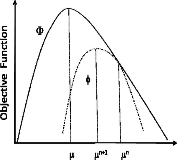
Illustration of the Optimization transfer principle in 1D.
c) Separable Paraboloidal Surrogates
The non-quadratic objective function is replaced by a surrogate function and one of the many possible surrogate functions suggested by Fessler et. al. is a surrogate paraboloidal function [7]. The curvature of this surrogate function determines the speed of convergence of the algorithm. Smaller curvature would mean more steps of iteration to reach the maximizer of the objective function. However the curvature of the surrogate function should be small enough such that the surrogate function lies below the objective function. The surrogate of the objective function in Eqn. 1 can be written as
| (8) |
Where QL can be defined as the surrogate of the log-likelihood function if ϕ satisfies the 3 condition in Eqn 5–7. A difficulty in maximizing Eqn. 8 is that both Q and R are nonseparable functions of the elements of the parameter vector μ. However Fessler et. al uses De Pierro's concavity trick [45] to form a second separable surrogate function. The details of the derivation can be seen in [7]. The final simplified form of the update equation can be written as
| (9) |
Where and are the derivative and the curvature of the surrogate function for the likelihood part and and are the derivative and the curvature of the penalty part.
2.5 Reconstruction Parameters for PML
The reconstruction parameters of interest are the penalty weight β and the edge preserving parameter δ. For the purpose of this paper, the parameters for the PML were optimized by visual examination of a set of images and β =10 and δ=0.001 were the chosen values. Higher values of β leads to smoother images, making it difficult to detect MCCs. Fig 3 compares image slices reconstructed using β values of 10, 1000 and 106. It is clear that a very high value of β leads to unacceptably smooth images.
Fig. 3.

Reconstructed images using PML with δ= 0.001 and (a) β =10.0 (b) β=10 (c) β =106
The PML reconstructions were run to convergence as defined by visual inspection and comparing the difference image after every ten iteration. To determine the number of iterations required for convergence, we examined images obtained at every 10 iterations up to a limit of 130 iterations. Results from iterations 10, 40, 80 and 100 are compared in Fig. 4. It was seen that more than 80 iterations gave little or no qualitative improvement in the images.
Fig. 4.

Reconstructed image with PML showing (a) 10 iterations (b) 40 iterations (c) 80 iterations (d) 100 iterations, all with δ = 0.001 and β =10.0
2.6 Comparison of PML and FBP
The visibility of MCs in the breast tomosynthesis image is influenced by factors such as acquisition dose, breast density and location of the MC cluster. A lower acquisition dose results in noisier projections and hence noisier reconstructions. For our comparison studies we simulated 3 different acquisition dose levels; 1.5 mGy, 1.0 mGy and 0.7 mGy. In order to evaluate observer performance, sets of images were reconstructed using both PML and FBP techniques from the same projection sets.
MC visibility in FBP images could change depending on the cut-off frequency used in the post-reconstruction 3D Butterworth filtering. Visually, a cut-off frequency of 0.25 pixel−1 produced smoother, more-appealing images at most dose levels, but it was found from the pilot observer study that higher cut-offs preserved the high-frequency information needed for better MC detection. Fig.5. shows a plot of the area under the LROC curve (AL) vs the cutoff frequency of 3D BW filtering for acquisition dose levels of 0.7, 1.0 and 1.5 mGy. For each dose level, the images that yielded the highest AL were chosen to be compared against the corresponding images generated using PML. Fig. 5 shows that the Butterworth cutoff frequencies yielding the highest AL for MC detectability were 0.45, 0.4 and 0.35 pixel−1 for the 0.7, 1.0 and 1.5 mGy dose levels, respectively. The images generated using these cutoff frequencies that yielded the best detectability was used for the corresponding dose levels for comparison with PML. It is interesting to note that the heavier filtering seemed optimum for higher dose level in comparison to the lighter filtering at lower dose level. This is counter intuitive to the fact that lower dose levels are more noisy and heavier filtering is generally desirable. One possible explanation for our data is that the nature of the noise texture at higher dose levels had more impact on the MC detectability (due to the MC size range and appearance) and hence required heavier filtering as opposed to the lower dose level cases. This aspect will be examined with a larger study in future with various MC sizes.
Fig. 5.
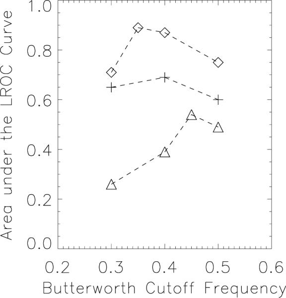
Area under the LROC vs Butterworth cutoff frequency (in pixel–1) FBP plotted for acquisition dose levels of 0.7 mGy (Triangle symbol), 1.0 mGy (plus symbol) and 1.5 mGy (Diamond symbol).
Fig. 6 shows PML and FBP reconstructed images simulated using 3 different breast phantoms of different densities for an acquisition dose level of 1mGy. Also shown is a zoomed region of interest (ROI) showing the MCC. From these zoomed ROI images, it is clear that visibility of the MC cluster depends on breast density and the location of the MCC within the breast. When the cluster is embedded in a dense background of fibro-glandular tissue, the visibility is reduced, whereas if the cluster is embedded within an adipose tissue region, visibility is improved. Fig. 6c shows MC in a low density breast and the cluster is embedded in adipose region making it easy to visualize using both the reconstruction techniques while Fig. 6a and 6b shows MC embedded in relatively high density breast volume (i.e surrounded by fiberoglandular tissue).
Fig. 6a.


Reconstructed image slices simulated with 1 mGy dose for (a) breast model 1 with PML reconstruction (left) and FBP (right) (b) breast model 2 with PML reconstruction (left) and FBP (right) (c) breast model 3 with PML reconstruction (left) and FBP (right).
An LROC analysis was used for comparing the performance of the two reconstruction techniques. The figure of merit used to assess performance was the area under the LROC curve (AL). Each LROC study consisted of the observer first reading a set of training images with feedback, followed by the study images. The observer's task was to localize the abnormality within the displayed image and give a confidence rating for each image. Four confidence ratings were used; 1) high confidence lesion present, 2) low confidence lesion present, 3) low confidence lesion absent and 4) high confidence lesion absent. If for a given displayed image, the observer was confident that there was no abnormality present, they were instructed to click on an arbitrary location within the image and select rating 4. If the observer suspected an abnormality at a certain location, they were instructed to click on the center of the abnormality and choose one of the three ratings from 1, 2 or 3. Each study set consisted on 96 study images and 20 training images. Four medical physicist observers participated in each of these study sessions. Before conducting each reading session, each observer was required to undergo training in reading images for the method to be evaluated. During this training session, feedback was provided to the reader after each selection. Immediately after the training session was completed, the comparison study was performed. The observer confidence rating and the suspected MCC location were recorded for all the images displayed. Swensson's method [46] was used to fit the data and obtain the area under the LROC curve using Swensson's software.
A two-way Analysis of Variance (ANOVA) [47] study was performed to estimate the statistical significance of the differences in techniques and also to estimate the statistical significance in the performance difference between the four observers.
3. RESULTS
This study compared MC detection accuracy obtained with two reconstruction methods; 1) a statistical iterative reconstruction method, using a penalized maximum likelihood objective function and 2) a more conventional filtered backprojection method. For each acquisition dose of 1.5 mGy, 1.0 mGy and 0.7 mGy, separate LROC studies were conducted to estimate the performance of MC detectability with both reconstruction strategies. Fig. 7 shows the LROC curve averaged over the four observers for both PML and FBP techniques shown for dose levels of 1.5 mGy (Fig. 7a), 1.0 mGy (Fig. 7b) and 0.7 mGy (Fig. 7c).
Fig. 7.

Comparing the average LROC curves for all four observers for PML (dashed) vs FBP(solid) for (a) 1.5 mGy acquisition (b) 1 mGy acquisition and (c) 0.7 mGy acquisition.
In all of these cases the sensitivity and specificity obtained using the PML technique was higher than that using FBP. Table 1 lists the average area under the LROC curve for the four observers for all three dose levels. The average area under the LROC curve for the dose of 1.5 mGy was 1.0 ± 0.00 for PML and 0.9 ± 0.014 for FBP, for the dose of 1.0 mGy it was 0.93 ± 0.05 for PML and 0.7 ± 0.07 or FBP and for the dose of 0.7 mGy it was 0.69 ± 0.06 for PML and 0.43 ± 0.04 for FBP. The uncertainties represent the standard deviation in observer performance. A two way ANOVA found statistically significant difference (at a significance level of 0.05) between the two reconstruction strategies for all three imaging dose levels with a p value = 0.0007 for the dose of 1.5 mGy, p= 0.014 for the dose level of 1.0 mGy and p=0.028 for the dose level of 0.7 mGy. There was no statistically significant difference (at a significance level of 0.05) in observer performance for each study with a p value = 0.5 for the dose of 1.5 mGy, p=0.48 for the dose of 1.0 mGy, p=0.7 for the dose of 0.7 mGy.
Table 1.
| AL for PML | AL for FBP | |
|---|---|---|
| 1.5 mGy acquisition | 1.0 ± 0.00 | 0.9 ± 0.014 |
| 1.0 mGy acquisition | 0.93 ± 0.05 | 0.7 ± 0.07 |
| 0.7 mGy acquisition | 0.69 ± 0.06 | 0.43 ± 0.04 |
4. DISCUSSIONS
The visualization of microcalcifications is important for detection of ductal carcinoma in situ (DCIS). It has been estimated that DCIS represents 30% of all breast cancer identified by screening mammography [48]. Since 30%–50% of all DCIS eventually become invasive [48], detection of DCIS is important and can contribute to a decreased breast cancer mortality rate. With conventional mammography, Feig [49] and Anderson [50] have reported that 89% and 95%, respectively, of DCIS were observed based on the presence of MCs alone. Another study [51] put the figure at 72%.
The conspicuity of MCs in DBT has been questioned. Poplack et al. [1] reported an initial experience with DBT by imaging 98 women with abnormal screening mammography. They reported that of the 11 cases in which DBT was inferior to screen-film mammography, 8 were exhibiting MCs. There are many possible reasons why DBT might not portray MCs on par with conventional mammography. This finding, as well as other anecdotal evidence, suggests that better MC detection with DBT might follow from improvements in the DBT technology. Our study indicates that iterative PML reconstruction is one such improvement.
In this paper we performed a comparison of the standard FBP reconstruction method with a PML reconstruction technique for MC detection in DBT. Human psychophysical studies conducted for three different dose levels show statistically significant improvement using the PML reconstruction. For the simulated dose levels of 1.5 mGy, the area under the LROC curves were 1.0 ± 0.00 for PML and 0.9 ± 0.014 for FBP, for the dose of 1.0 mGy it was 0.93 ± 0.05 for PML and 0.7 ± 0.07 or FBP and for the dose of 0.7 mGy it was 0.69 ± 0.06 for PML and 0.43 ± 0.04 for FBP. The differences are statistically significant for all three simulated dose levels.
This study used simulated images generated from an accurate model of the DBT imaging process. This model includes the use of anthropomorphic, compressed breast phantoms with realistic anatomical noise. In addition, the physics of photon transport through the indirect conversion, CsI-based detector were modeled. The imaging model did not include the effects of scattered radiation, but since both reconstruction methods operated on the same projection sets, we hypothesize that the addition of scatter would not have altered the results of our comparison study. There are many methodological advantages in comparing reconstruction methods using realistically simulated data. However, further evaluation studies using clinical data should also be conducted.
The current study was performed with individual 2D slices extracted from 3D image volumes. The display threshold levels were preset for the observer, with the threshold selected by the investigators on the basis of subjective MC appearance. One possible improvement for the study methodology would be to use 3D volumes and allow the observer to scan through the 2D slices, changing the display threshold for each slice. To fully evaluate the reconstruction methods for clinical use, the detectability of low-contrast, mass-like structures also must be considered. The Butterworth filtering parameters employed here for FBP may not be the best choice for mass detectability. For FBP, the parameters of the Butterworth post-reconstruction filter were determined from LROC pilot studies. In future studies, these cut off frequencies would be examined more closely for various calcification sizes and dose levels of acquisitions. The parameters for PML reconstruction were chosen based on visual inspection. Complete optimization of PML parameters using human observer studies would be very time consuming due to multiple parameters that need to be optimized. While an optimization of PML parameters would likely lead to larger performance differences between the two methods, these pilot studies would be very time intensive because it is a 2D parameter space. To this end we are developing a model observer (MO) whose performance would match that of human observer performance. Such a MO could be used for optimization of reconstruction and acquisition parameters.
PML reconstruction was iterated until convergence to avoid having iteration number as a variable. It is possible that lower number of iterations would have yielded similar results (in terms of detectability of MCC). The number of iterations needed for convergence depends on the curvature of the surrogate parabola chosen in the SPS technique used to solve the PML problem. This is one of the factors which could use more investigations and may help to speed up convergence.
A very high value of penalty strength β yields a blurry image and low visibility of MCCs. The choice of appropriate δ depends on the edge-preserving effect that one desires at the boundaries of two tissue type. This in turn depends on the differences in the attenuation properties of the tissue types that are in the region of interest. For our particular work focusing on MC detection, the important edges were boundaries separating MCs and the surrounding adipose and fibro-glandular tissue. With transmission imaging, one has some prior knowledge in the form of the average attenuation coefficients of these tissues. For the purpose of this study we did not account for this knowledge, based on the fact that tomosynthesis yields blurry image and does not accurately reconstruct the attenuation values due to incomplete sampling of the data space (here only 21 projections acquired over a total 60 degree arc). Note that the reconstruction method we used do not account for the energy dependence of the attenuation coefficients. Hence only an effective attenuation value is being reconstructed. The image is heavily blurred in the plane parallel to the x-ray beam at 0th angle (z-direction). Thus only the orthogonal plane in the 3D image is informative. In calculating the weights (See Eqn. 2) for the penalty function, neighboring pixels in all 3 dimensions were considered for our simulation. Ignoring the neighboring pixels in the z direction for calculating the weights did not seem to change the results. This could be due to the fact that the image is heavily blurred in this direction and including the neighbors in this direction does not contribute significantly to the weight calculation. An extensive study working on various combinations of parameters varying within a wide range will be needed before one could optimize the parameters for best performance for a given task (such as MC detectability or mass detectability) in tomosynthesis.
Finally, we note that the PML algorithm used herein is computationally intensive for DBT. In this study, little effort was made to optimize the computer implementation of the algorithm. Future work will consider a number of possible techniques for reducing computation time (currently about 24 hours for 80 iterations on a single CPU), including the use of graphics processor units and parallel processors [15].
5. CONCLUSIONS
For all three acquisition dose levels considered, the PML reconstructions yielded higher detection accuracy of MCCs compared to FBP. The difference in performance at each dose was statistically significant. As the dose level was decreased, the performance difference between the two algorithms increased, indicating that the PML algorithm may be especially beneficial at lower acquisition doses. These results indicate that PML algorithm shows better dose efficiency than FBP. Continued studies with optimized PML parameters, improved psychophysical experiments using 3D display of images and more number of observers and test cases need to be performed.
Acknowledgements
We thank Dr. Souleyman Konate (Department of Radiology, UMMS) and Mr. Kesava Kalluri (Dept. of Radiology at UMMS/ECE at UML) for participating in the observer study. This work was supported in part by the National Institutes of Health (NIH) under Grants NIH-K25CA140858-01 and R01 CA102758 from the National Cancer Institute (NCI). Its contents are solely the responsibility of the authors and do not necessarily represent the official views of the NIH or the NCI.
REFERENCES
- 1.Poplack SP, Tosteson TD, Kogel CA, Nagy HM. Digital Breast Tomosynthesis: Initial Experience in 98 Women with Abnormal Digital Screening Mammography. AJR. 2007;189:616–623. doi: 10.2214/AJR.07.2231. [DOI] [PubMed] [Google Scholar]
- 2.Kopans D, Moore R, Gavenonis S. Calcification in digital breast tomosynthesis. RSNA 2008,Session SSJ01-02 Breast Imaging (digital/tomosynthesis); [DOI] [PubMed] [Google Scholar]
- 3.Feldkamp LA, Davis LC, Kress JW. Practical cone-beam algorithm. J. Opt. Soc. Am. 1984;1:612–619. [Google Scholar]
- 4.Mertelmeier T, Orman J, Haerer W, Dudam MK. Optimizing fileterd backprojection reconstruction for a breast tomosynthesis prototype device. Proceedings of SPIE: Physics of Medical Imaging. 2006;6142(61420F) [Google Scholar]
- 5.Zhou J, Zhao B, Zhao W. A computer simulation platform for optimization of a breast tomosynthesis system. Med. Phys. 2007;34(3):1098–1108. doi: 10.1118/1.2558160. [DOI] [PubMed] [Google Scholar]
- 6.Wu T, Moore RH, Rafferty EA, Kopans DB. A comparison of reconstruction algorithms for breast tomosynthesis. Med. Phys. 2004;31(9):2636–2647. doi: 10.1118/1.1786692. [DOI] [PubMed] [Google Scholar]
- 7.Fessler JA. Statistical image reconstruction methods for transmission tomography. In: Sonka M, Fitzpatrick JM, editors. Handbook of Medical Imaging, Volume 2. Medical Imaging Processing and Analysis. SPIE; Bellingham: 2000. [Google Scholar]
- 8.Zhang Y, et al. A comparitive study of limited angle cone-beam reconstrcution methods for breast tomosynthesis. Medical Physics. 2006;33(10):3781–95. doi: 10.1118/1.223754. [DOI] [PMC free article] [PubMed] [Google Scholar]
- 9.Sidky EY, Pan X, Reiser IS, Nishikawa RM, Moore RH, Kopans D. Enhanced imaging of microcalcifications in digital breast tomosythesis through improved image-reconstruction algorithms. Medical Physics. 2009;36(11):4920–4932. doi: 10.1118/1.3232211. [DOI] [PMC free article] [PubMed] [Google Scholar]
- 10.Elbakri AI, Fessler JA. Statistical image reconstruction for polyenergetic X-ray computed tomography. IEEE Transactions on Med. Imag. 2002;21(2):89–99. doi: 10.1109/42.993128. [DOI] [PubMed] [Google Scholar]
- 11.Gifford HC, King MA, Wells RG, Hawkins WG, Narayanan MV, Pretorius PH. LROC analysis of detector-response compensation in SPECT. IEEE Transactions on Med. Imag. 2000;19:464–463. doi: 10.1109/42.870256. [DOI] [PubMed] [Google Scholar]
- 12.Gilland DR, Tsui BMW, Metz CE, Jaszczak RJ, Perry JR. An evaluation of maximum likelihood-expectation maximization reconstruction for SPECT by ROC analysis. The Journal of Nuclear Medicine. 1992;33:451–457. [PubMed] [Google Scholar]
- 13.Wang J, Li T, Xing L. Iterative image reconstrcution for CBCT using edge-preserving prior. Med. Phys. 2009;36(1):252–260. doi: 10.1118/1.3036112. [DOI] [PMC free article] [PubMed] [Google Scholar]
- 14.Nuyts J, Beque D, Dupont P, Mortelmans L. A concave prior penalizing relative differences for maximum-a-posteriori reconstruction in emission tomography. IEEE Transactions on nuclear science. 2002;49(1):56–60. [Google Scholar]
- 15.Sotthivirat S, Fessler JA. Image recovery using partitioned-separable paraboloidal surrogatecoordinate ascent algorithms. IEEE Transactions on image processing. 2002;11(3):306–317. doi: 10.1109/83.988963. [DOI] [PubMed] [Google Scholar]
- 16.Delaney AH, Bresler Y. Globally convergent edge-preserving regularized reconstrcution: An application to limited-angle tomography. IEEE Transactions on image processing. 1998;7(2):204–221. doi: 10.1109/83.660997. [DOI] [PubMed] [Google Scholar]
- 17.Bouman CA, Sauer K. A unified approach statistical tomography using coordinate decent optimization. IEEE Transactions on image processing. 1996;5:480–492. doi: 10.1109/83.491321. [DOI] [PubMed] [Google Scholar]
- 18.Chawla AS, Lo JY, Baker JA, Samei E. Optimized image aquisition for breast tomosynthesis in projection and reconstruction space. Medical Physics. 2009;36(11):4859–4869. doi: 10.1118/1.3231814. [DOI] [PMC free article] [PubMed] [Google Scholar]
- 19.Hu Y, Zhao W, Mertelmeier T, Ludwig J. Image artifact in digital breast tomosynthesis and it dependence on system and reconstruction parameters. Lecture Notes in Computer Science. 2008;5116:628–634. [Google Scholar]
- 20.Zhang Y, et al. A comparitive study of limited-angle cone-beam reconstrcution methods for breast tomosynthesis. Medical Physics. 2006;33(10):3781–3795. doi: 10.1118/1.223754. [DOI] [PMC free article] [PubMed] [Google Scholar]
- 21.Boone JM, Fewell TR, Jennings RJ. Molybdenum, rhodium, and tungsten anode spectral models using interpolating polynomials with application to mammography. Med. Phys. 1997;24(12):1863–1874. doi: 10.1118/1.598100. [DOI] [PubMed] [Google Scholar]
- 22.Boone JM. Glandular Breast Dose for monoenergetic and high-energy x-ray beams: Monte Carlo assessment. Radiology. 1999;213:23–37. doi: 10.1148/radiology.213.1.r99oc3923. [DOI] [PubMed] [Google Scholar]
- 23.Siewerdsen JH, Jaffray DA. Optimization of x-ray imaging geometry (with specific application to flat-panel cone-beam computed tomography) Med. Phys. 2000;27(8):1903–1914. doi: 10.1118/1.1286590. [DOI] [PubMed] [Google Scholar]
- 24.Siddon RL. Fast calculation of the exact radiological path for a three-dimensional CT array. Med. Phys. 1985;12(2):252–255. doi: 10.1118/1.595715. [DOI] [PubMed] [Google Scholar]
- 25.Vedula AA, Glick SJ, Gong X. Computer simulation of CT mammography using a flat-panel imager. SPIE Physics of Medical Imaging. 2003;vol. 5030:349–360. [Google Scholar]
- 26.Siewerdsen JH, Antonuk LE, et al. Empirical and theoretical investigation of the noise performance of indirect detection, active matrix flat-panel imagers (AMFPIs) for diagnostic radiology. Med. Phys. 1997;24(1):71–89. doi: 10.1118/1.597919. [DOI] [PubMed] [Google Scholar]
- 27.Vedantham S, Karellas A, Suryanarayanan S, et al. Full breast digital mammography with an amorphous silicon-based flat panel detector: Physcial characteristics of a clinical prototype. Med Phys. 2000;27:1–10. doi: 10.1118/1.598895. [DOI] [PMC free article] [PubMed] [Google Scholar]
- 28.Mainprize JG, Bloomquist AK, Kempston MP, Yaffe MJ. Resolution at oblique incidence angles of a flat panel imager for breast tomosynthesis. Medical Physics. 2006;33(9):3159–3164. doi: 10.1118/1.2241994. [DOI] [PubMed] [Google Scholar]
- 29.O'Connor JM, Glick SJ, Gong X, Didier CS, Mah'd M. Characterization of a prototype table-top x-ray CT breast imaging system. SPIE Medical Imaging. 2007;vol. 6510 [Google Scholar]
- 30.O'Connor JM, Das M, Didier C, Mah'D M, Glick SJ. Medical Imaging 2008: Physics of Medical Imaging. SPIE; San Diego, CA, USA: 2008. Using mastectomy specimens to develop breast models for breast tomosynthesis and CT breast imaging. [Google Scholar]
- 31.O'Connor JM, Das M, Didier C, Mah'D M, Glick SJ. International Workshop on Digital Mammography (IWDM) Lecture notes in computer science (Springer); Girona, Spain: Jun, 2010. Development of an ensemble of digital breast object models. [Google Scholar]
- 32.Altunbas MC, et al. A post-reconstruction method to correct cupping artifacts in one-beam breast computed tomography. Med. Phys. 2007;34(7) doi: 10.1118/1.2748106. [DOI] [PMC free article] [PubMed] [Google Scholar]
- 33.Perona P, Malik J. Scale-space and edge detection using anisotropic diffusion. IEEE Transactions on Pattern Analysis and Machine Intelligence. 1990;12(7) [Google Scholar]
- 34.Das M, Gifford H, O'Connor M, Glick S. SPIE Medical imaging: Physics of Medical Imaging(6913) SPIE; San Diego, CA, USA: 2008. Evaluation of a variable dose acquisition methodology for breast tomosynthesis. [DOI] [PMC free article] [PubMed] [Google Scholar]
- 35.Das M, O'Connor JM, Gifford HC, Glick SJ. Evaluation of a variable dose aquisition technique for microcalcification and mass detection in digital breast tomosynthesis. Medical Physics. 2009;36:1976–1984. doi: 10.1118/1.3116902. [DOI] [PMC free article] [PubMed] [Google Scholar]
- 36.O'Connor JM, Das M, Didier C, Mah'D M, Glick SJ. Development of an ensemble of digital breast object model. Lecture Notes in Computer Science (IWDM2010) 2010;6136:54–61. [Google Scholar]
- 37.Carton A, Currivan JA, Conant E, Maidment A. Temporal subraction versus dual-energy contrast enhanced digital breast tomosynthesis : A pilot study. Lecture Notes in Computer Science. 2008;5116:163–173. [Google Scholar]
- 38.Yaffe MJ, et al. The myth of 50–50 breast. Med. Phys. 2009;36:5437. doi: 10.1118/1.3250863. [DOI] [PMC free article] [PubMed] [Google Scholar]
- 39.Tonge KA, Davis R, Millis RR. The poblem of discrimination in mammography. Arguments for using a biological test objects. British J. Radiology. 1976;49:678–685. doi: 10.1259/0007-1285-49-584-678. [DOI] [PubMed] [Google Scholar]
- 40.Wheeler FW, Perera AG, Claus BE, Muller SL, Peters G, Kaufhold JP. Micro-calcification detection in digital tomosynthesis mammography. SPIE Medical Imaging Proceedings. 2006;6144(Part1):614420. [Google Scholar]
- 41.Ruschin M, et al. Dose dependence of mass and microcalcification detection in digital mammography: Free response human observer studies. Med Phys. 2007;34:400–407. doi: 10.1118/1.2405324. [DOI] [PMC free article] [PubMed] [Google Scholar]
- 42.Johns PC, Yaffe MJ. X-ray characterisation of normal and neoplastic breast tissues. Phys. Med. Biol. 1987;32(6):675–695. doi: 10.1088/0031-9155/32/6/002. [DOI] [PubMed] [Google Scholar]
- 43.Gong X, Vedula AA, Glick SJ. Microcalcification detection using cone-beam CT mammography with a flat-panel imager. Phys. Med. Biol. 2004;49(11):2183–2195. doi: 10.1088/0031-9155/49/11/005. [DOI] [PubMed] [Google Scholar]
- 44.Chen B, Ning R. Cone-beam volume CT breast imaging: Feasibility study. Med. Phys. 2002;29(5):755–770. doi: 10.1118/1.1461843. [DOI] [PubMed] [Google Scholar]
- 45.De Pierro AR. A modified expectation maximization algorithm for penalized likelihood estimation in emission tomography. IEEE Transactions on Med. Imag. 1995;14:132–137. doi: 10.1109/42.370409. [DOI] [PubMed] [Google Scholar]
- 46.Swensson RG. Unified measurement of observer performance in detecting and localizing target objects on images. Med. Phys. 1996;23(10):1709–1725. doi: 10.1118/1.597758. [DOI] [PubMed] [Google Scholar]
- 47.Pollard JH. A handbook of numerical and statistical techniques. Cambridge univ. press; Cambridge: 1977. [Google Scholar]
- 48.Kopans DB. Breast Imaging. 2nd ed. Lippincott, Williams, and Wilkins; Philadelphia: 1998. [Google Scholar]
- 49.Feig SA, Shaber GS, Patchefsky A. Analysis of clinically occult and mammographically occult breast tumors. AJR. 1977;128:403–408. doi: 10.2214/ajr.128.3.403. [DOI] [PubMed] [Google Scholar]
- 50.Anderson I. Ph.D. Thesis. Malmo: 1980. Mammographic screening for breast carcinoma. [Google Scholar]
- 51.Stomper PC, Connolly JL, Meyer JE, Harris JR. Clinically occult ductal carcinoma in situ detected with mammography: analysis of 100 cases with radiologic-pathologic correlation. Radiology. 1989:235–241. doi: 10.1148/radiology.172.1.2544922. [DOI] [PubMed] [Google Scholar]