Patterns and Evolution of Nucleotide Landscapes in Seed Plants

Laurana Serres-Giardi; Khalid Belkhir; Jacques David; Sylvain Glémin

doi:10.1105/tpc.111.093674

. 2012 Apr 6;24(4):1379–1397. doi: 10.1105/tpc.111.093674

Patterns and Evolution of Nucleotide Landscapes in Seed Plants^{^[W]}

Laurana Serres-Giardi ^a,^b, Khalid Belkhir ^a, Jacques David ^b, Sylvain Glémin ^a,¹

PMCID: PMC3398553 PMID: 22492812

Analysis of EST sequence data in more than 200 species reveals unexpected continuous variations in GC content in seed plant genomes, with several independent enrichment episodes from GC-poor and homogeneous genomes to more derived GC-rich and highly heterogeneous ones. It reveals the possible role of GC-biased gene conversion, a recombination-associated process favoring G and C bases.

Abstract

Nucleotide landscapes, which are the way base composition is distributed along a genome, strongly vary among species. The underlying causes of these variations have been much debated. Though mutational bias and selection were initially invoked, GC-biased gene conversion (gBGC), a recombination-associated process favoring the G and C over A and T bases, is increasingly recognized as a major factor. As opposed to vertebrates, evolution of GC content is less well known in plants. Most studies have focused on the GC-poor and homogeneous Arabidopsis thaliana genome and the much more GC-rich and heterogeneous rice (Oryza sativa) genome and have often been generalized as a dicot/monocot dichotomy. This vision is clearly phylogenetically biased and does not allow understanding the mechanisms involved in GC content evolution in plants. To tackle these issues, we used EST data from more than 200 species and provided the most comprehensive description of gene GC content across the seed plant phylogeny so far available. As opposed to the classically assumed dicot/monocot dichotomy, we found continuous variations in GC content from the probably ancestral GC-poor and homogeneous genomes to the more derived GC-rich and highly heterogeneous ones, with several independent enrichment episodes. Our results suggest that gBGC could play a significant role in the evolution of GC content in plant genomes.

INTRODUCTION

The nucleotide landscape, which is the way base composition varies along a genome, is a striking characteristic of genome organization that strongly varies among species. In eukaryotes, the mean GC content varies from ~20 to 60% (Lynch, 2007). In some species, such as humans, the base composition is highly heterogeneous, and genomes appear as patchworks of GC-rich and GC-poor regions at the 100-kb scale (Lander et al., 2001). This peculiar feature of base composition variation was called isochore structure after its discovery by ultracentrifugation (Bernardi et al., 1985). It has been well described in other vertebrates, especially in mammals and birds (reviewed in Eyre-Walker and Hurst, 2001). In these groups, the GC content varies locally and correlations are found on a small scale among GC content in coding, introns, and flanking regions (Aïssani et al., 1991) as well as among GC content in the first, second, and third codon positions (GC1, GC2, and GC3 hereafter) (Clay et al., 1996). Strikingly, other genome characteristics are associated with GC content: For instance, in GC-rich regions, gene density is higher and genes are more compact (shorter introns) (Mouchiroud et al., 1991). Recombination (Fullerton et al., 2001; Duret and Arndt, 2008), expression level (Kudla et al., 2006), and replication timing (Costantini and Bernardi, 2008) were also shown to correlate with GC content.

The evolutionary causes of isochore structure, in particular the existence of GC-rich isochores, have been much debated. The initial hypothesis of adaptation to homeothermy (Bernardi et al., 1985) has been ruled out for several reasons, including the discovery of GC-rich isochores in some reptiles, which are not homeothermic (Hughes and Mouchiroud, 2001). Three main hypotheses, not mutually exclusive, are now commonly proposed to explain nucleotide landscape evolution: selection on codon usage (SCU) in coding regions, mutational bias (MB), and GC-biased gene conversion (gBGC) (reviewed in Eyre-Walker and Hurst, 2001; Duret and Galtier, 2009). Selection for the accuracy of translation can affect synonymous codon usage (reviewed in Akashi, 2001). The GC content of coding sequences (CDSs), especially in the third codon position, could thus be driven by translational selection.

Under the SCU hypothesis, highly expressed genes are expected to undergo stronger translational selection, hence higher GC contents, if preferred codons mainly end in G or C. Variation in translational selection intensity among genes could explain within-genome variations in GC content, and variations in codon usage preferences could explain differences in GC content between species. Nevertheless, the SCU hypothesis cannot explain the GC content variations in noncoding regions and in nonsynonymous positions.

The MB hypothesis stipulates that GC content is driven by variation in MB along the genome, which can explain GC content variations at all codon positions. Several kinds of MBs have been suggested. They include variation in bias associated with replication timing due to variations in free nucleotide availabilities during the cell cycle (Wolfe et al., 1989) and the negative effect of the local GC content on the rate of cytosine deamination, which is the major cause of C→T and G→A mutations. The latter mechanism would drive either impoverishment or enrichment in GC content in a positive feedback (Fryxell and Zuckerkandl, 2000). However, MB hypotheses were seriously weakened by polymorphism data. Several studies revealed that the mutational pattern was biased toward AT mutations and that a bias of fixation occurred in favor of GC alleles, a typical selection-like signature (e.g., Galtier et al., 2001; Smith and Eyre-Walker, 2001; Katzman et al., 2011).

Since the last decade, the gBGC hypothesis has increasingly been recognized as the main force driving GC content evolution in mammalian genomes and in other taxonomic groups (reviewed in Duret and Galtier, 2009). gBGC is a recombination-associated process that favors GC over AT bases in alleles during mismatch repair following heteroduplex formation at meiosis (reviewed in Marais, 2003). Because this process mimics selection (Nagylaki, 1983), the gBGC hypothesis is compatible with both selection-like signatures (contrary to the MB hypothesis) and with genome-wide effects (contrary to the SCU hypothesis). Moreover, as gBGC is driven by recombination, the strong correlations between recombination and GC content and GC substitution patterns are well predicted by this hypothesis (Meunier and Duret, 2004; Duret and Arndt, 2008). Isochore structure can thus be explained by the heterogeneity of recombination throughout the genome (Duret and Galtier, 2009).

As opposed to vertebrates, the base composition has only been investigated in a few plant species (e.g., Carels and Bernardi, 2000; Tatarinova et al., 2010) mainly focused on the comparison between rice (Oryza sativa) and Arabidopsis thaliana (e.g., Wong et al., 2002; Wang et al., 2004; Guo et al., 2007; Wang and Hickey, 2007). Gene GC content appeared to be heterogeneous, especially in grasses that exhibit a bimodal GC3 distribution, as opposed to other species studied so far (Carels and Bernardi, 2000; Wang et al., 2004; Tatarinova et al., 2010). In Arabidopsis, the correlation between GC3 and GC content of flanking regions suggested a similar isochore structure as in vertebrates (Barakat et al., 1998). Based on only several genes, such local correlations were also suggested to occur in other plants, including grasses (Matassi et al., 1989). However, a recent study in rice showed that GC3 is correlated to GC1, GC2, and GC in introns, as initially suggested, but not to flanking (1 kb) sequences (Tatarinova et al., 2010). This suggests that GC content could be structured at a very local scale around genes and/or that transposable element dynamics might have disrupted local correlations. Note that in mammals, the GC content correlation between third positions and flanking sequences is weak when using all genes (Elhaik et al., 2009) but much more clear when using orthologous more highly conserved genes (Romiguier et al., 2010). In rice, GC content was also found to strongly decrease from 5′ to 3′ along genes, whereas this GC gradient is much weaker in Arabidopsis (Wong et al., 2002). These striking differences between rice and Arabidopsis have been extended to few other eudicots species, including Brassica sp, pea (Pisum sativum), potato (Solanum tuberosum), tomato (Solanum lycopersicum), tobacco (Nicotiana tabacum), soybean (Glycine soja), and sunflower (Helianthus annuus), and other grasses, including barley (Hordeum vulgare), maize (Zea mays), oat (Avena sativa), sorghum (Sorghum bicolor), and wheat (Triticum aestivum), and are often generalized as a dicots/monocots dichotomy (e.g., Wong et al., 2002; Wang et al., 2004). This vision is clearly phylogenetically biased, and the peculiar pattern observed in Poaceae has not been observed in the few other monocots studied so far: GC content in onion (Allium cepa) is more similar to the one in Arabidopsis than in rice (Kuhl et al., 2004), and in banana (Musa spp), GC content appears intermediate between Arabidopsis and rice.

In addition, the mechanisms involved in GC content variations in plants are still weakly established, and most studies have exclusively focused on explaining the peculiar structure of Poaceae genomes. In rice and other grasses, most preferred codons end in G or C (Wang and Roossinck, 2006), suggesting that SCU can partly explain GC3 pattern in these species. However, the SCU hypothesis alone is not sufficient because weakly expressed genes also show a strongly bimodal GC3 distribution (Mukhopadhyay et al., 2007) and other positions are also affected (Carels and Bernardi, 2000; Shi et al., 2006). Other authors have thus invoked a general MB toward GC (Wang et al., 2004; Wang and Hickey, 2007). However, a recent study ruled out this hypothesis in rice by showing that, as in mammals, mutation is AT biased and fixation GC biased (Muyle et al., 2011). Finally, as in mammals and birds, gBGC was suggested to affect GC content in grasses (Glémin et al., 2006; Haudry et al., 2008; Escobar et al., 2010; Muyle et al., 2011), but we know very little on the possible occurrence of gBGC in other plant species (but see Wright et al., 2007).

Our view of both the patterns and the process of GC content evolution in plant genomes is thus very scattered. We do not know whether GC-rich and heterogeneous gene content is a specific property of grasses or whether it is shared with other monocots. We ignore whether all eudicots have GC-poor and homogeneous genomes or not. The ancestral nucleotide landscape of angiosperms remains unknown. In addition, we do not know whether the underlying mechanisms differ between groups. We thus clearly need a broader phylogenetic view of GC-content variations in flowering plants. As a comparison, even in well-studied groups as mammals, a recent study extending GC content analyses from six to eight to 33 complete genomes substantially modified the view of isochore dynamics and pinpointed the role of life history traits (body mass and longevity) and genome size on isochore evolution (Romiguier et al., 2010). In plants, there are currently too few complete genomes available, and key phylogenetic groups are still lacking (e.g., basal angiosperms, nongrass monocots, and asterids). Recently, Escobar et al. (2011) used an alternative approach and analyzed only one gene (18S rDNA) in more than 1000 angiosperm species. They showed that 18S rDNA GC content had enriched within monocots (not only in Poaceae) and suggested that gBGC could explain this pattern. They argued that 18S rDNA GC content could be a good marker of the processes involved in GC content variations among species. Yet, the 18S rDNA is clearly not sufficient to characterize GC content distributions.

Here, we propose an intermediate approach using EST sequence data from 232 species covering most angiosperm clades, plus a few gymnosperms used as outgroups, to describe global base composition heterogeneities and explore local variations at the transcript scale within and across species. EST data allow characterizing GC content in many genes in a large phylogenetic sample. We provide the most comprehensive description of gene GC content in angiosperms and gymnosperms and specifically address the following questions. How are GC richness and base composition heterogeneity distributed across the phylogeny of seed plants? Are the genomic patterns observed in rice specific to Poaceae? What are the underlying mechanisms involved in the evolution of base composition? We find a continuous pattern of nucleotide landscapes from the possibly ancestral GC-poor and homogeneous genomes to the more derived GC-rich and highly heterogeneous genomes. The data strongly suggest that GC content enrichment occurred several times independently, especially among commelinid monocots. Finally, we discuss why the data appear more compatible with the gBGC hypothesis than with the alternative ones.

RESULTS

We characterized GC content distributions in 232 seed plant species (16 gymnosperms, six basal angiosperms, 56 monocots, and 154 eudicots) using a set of 3,435,183 EST unigenes. A unigene corresponds to the assembly of a set of transcript sequences that appear to come from the same transcription locus, representing the mature mRNA (or only a fragment) of an expressed gene. After assembly, annotation, and filtering (see Methods), each species data set contained at least 1000 sequences with more than 99 nucleotides. GC contents were analyzed separately for the different nucleotide positions: 5′ untranslated region (UTR; GC5UTR), 3′UTR (GC3UTR), first codon position (GC1), second codon position (GC2), and third codon position (GC3). We focused mainly on GC3. This is because most variations in the third coding position are synonymous and almost neutral or weakly selected. Therefore, GC3 should better reflect genome-wide variations in base composition. Results for all species are available in Supplemental Data Set 1 online.

Validation of EST Data by Comparison with Complete Transcriptome Data

Complete transcriptome sequences (i.e., the set of complete annotated CDS) of seven species (three dicots: Arabidopsis, poplar [Populus trichocharpa], and grape [Vitis vinifera]; and four grasses: Brachypodium distachyon, rice, sorghum, and maize) were used as controls to test whether EST data gave representative and unbiased results of all transcripts to describe the base composition patterns. Mean GC3 contents computed with complete transcriptomes were very similar to those computed with EST data (see Supplemental Data Set 2 online). Because many EST corresponded to gene fragments, sampling variance on GC content inflated the sds computed with EST data compared with those computed with complete genomes (see Supplemental Data Set 2 and Supplemental Figure 1 online). To tackle this problem, we modeled the GC content distributions and took sampling variance into account to fit the model to the data. To capture the heterogeneity of GC content distribution, especially the cases with bimodality, we assumed that GC content followed a bi-Beta distribution that is the mix of two BetaAU: distributions in proportions p and 1 – p with density function:

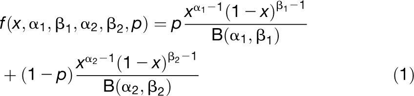graphic file with name PC.093674.lw.e1.jpg

where x is the GC content and B(α, β) is the Beta function (Abramowitz and Stegun, 1970). The use of two distributions is sufficient to obtain good fits and to give results with the simple biological meaning of two classes of genes regarding GC content (Carels and Bernardi, 2000). We fitted the five parameters of the bi-Beta using maximum likelihood (see Methods). Fitted parameters were used to obtain estimates of the mean and the sd of GC content distributions that (partly) correct for sampling variance. The estimated means of the bi-Beta fits were very close to the raw averages and the complete transcriptome averages (see Supplemental Data Set 2 online). For the whole species set, raw averages and bi-Beta means were also mostly identical (see Supplemental Figure 2 online; Spearman’s rho = 0.999, P value < 10⁻¹⁵). The estimated sds of the bi-Beta fits were lower than the raw sds and much more similar to the sds of the complete CDS sets than the raw sds (see Supplemental Data Set 2 online). However, though overestimated, raw sds were strongly correlated to the bi-Beta sds (see Supplemental Figure 2 online; Spearman’s nonparametric coefficient of correlation rho = 0.997, P value < 10⁻¹⁵). More generally, the GC3 bi-Beta distribution estimated through EST data was also similar to the full GC3 distribution obtained from whole-genome transcripts (see Supplemental Figure 1 online). Because estimates obtained through the bi-Beta distribution were closer to the full distribution than raw estimates, we chose to further use these corrected estimates instead of raw values. This approach also allowed us to characterize the properties of the two underlying distributions possibly corresponding to two classes of genes (see below).

Since we found the results for GC1 and GC2 to be similar to those for GC3 (see Supplemental Data Set 2 and Supplemental Figure 2 online), we also used corrected estimates for GC1 and GC2. GCUTR were more problematic because there were fewer sequences and they were shorter, which resulted in irregular raw distributions. For many species, we were thus not able to fit a bi-Beta distribution because of convergence problems during maximum likelihood maximization. We thus used the raw averages and sds. However, because raw and corrected averages and sds were highly correlated, relative results should be very similar. Moreover, raw means and sds were quite close to the transcriptome estimates (see Supplemental Data Set 2 online).

Finally, we verified that the size of the EST bank or the number of unigenes did not affect the results (see Supplemental Figure 3 online).

Strong Variation in GC Richness across the Seed Plant Phylogeny

We found strong variations in the mean GC content among species for all coding positions, with GC3 being the most contrasted (Figure 1). Unbiased mean GC3 ranged from 35.9% for the Papaveraceae species Eschscholzia californica to 68.2% for the Poaceae species Secale cereale (rye; see Supplemental Data Set 1 online). Phylogeny strongly impacts GC3 variations (Figure 1). To detect how variations in GC3 are distributed on the phylogeny, we estimated the variance component among six nested taxonomic levels (Table 1). We found that most variations (38.0%) occurred at the highest taxonomic level that included gymnosperms (mean GC3 = 42.4%), basal angiosperms (44.4%), monocots (55.8%), and eudicots (43.9%). Most of the variation was due to the difference between monocots and the other three groups (P values < 0.0001), whereas no significant difference was found between gymnosperms, basal angiosperms, and eudicots (Figure 2; see Supplemental Table 1 online). The rest of the variance mainly arose at the lower taxonomic levels, species (21.2%), family (18.9%), and genus (11.3%) (Table 1).

Table 1.

Variance Component Estimates (in %) of the Effect of Taxonomy on GC3 (Mean and sd)

Data Set	Statistics	Group	Infra Group	Super Order	Order	Family	Genus	Species
Total	Mean	38.0	0.0	8.6	2.0	18.9	11.3	21.2
	sd	52.1	0.0	10.6	0.0	13.5	12.0	11.8
Monocots	Mean	–	–	38.6	0.0	14.7	0.0	46.7
	sd	–	–	48.9	0.0	16.2	0.0	34.9
Eudicots	Mean	–	0.0	0.0	19.0	45.3	21.8	14.0
	sd	–	0.0	11.6	7.6	35.5	32.6	12.6

Open in a new tab

The variations in GC3 mean and sd are decomposed into the proportion due to every nested taxonomic level. For instance, for the full data set, 38% of mean GC3 variation is due to average differences among the four groups (gymnosperms, basal angiosperms, monocots, and eudicots), and 21.2% of variations are due to differences among species that are not attributable to higher taxonomic levels. Values for Group and Infra Group are not defined for the monocot data set because these taxonomic levels are higher than the monocot level and, hence, not nested within it. Similarly, values for Group are missing for the eudicot data set because these taxonomic levels are higher than the eudicot level.

We also found strong variations in the mean GC3 within monocots, from 40.0% in onion to 68.2% in S. cereale, and 38.6% of the variance was due to the difference between commelinids (mean GC3 = 58.2%) and other monocots (mean GC3 = 48.1%) (P value < 0.0001; Table 1; see Supplemental Table 1 and Supplemental Figure 4 online). Because grasses were known to have peculiar GC content (e.g., Carels and Bernardi, 2000; Wang et al., 2004), we also distinguished them from other commelinid species. Surprisingly, we also found significant differences at this level (mean GC3: Poaceae = 59.2%, other commelinids = 53.1%; P value = 0.0163). However, the major part of the variance (46.7%) is due to differences between species that are not due to higher taxonomic levels. This is well illustrated by the wide variation observed within grasses, from bamboo (Phyllostachis edulis) (mean GC3 = 46.9%) to rye (mean GC3 = 68.5%). Important variations also occurred in eudicots (from 35.9% in E. californica to 57.1% in Eucalyptus grandis), but variation was more evenly distributed among the different taxonomic levels (Table 1) and no clear phylogenetic pattern emerged (Figure 1; see Supplemental Figure 1 online). Some orders appeared much more GC rich than the average, such as Myrtales, whereas others were somewhat lower, such as Ranunculales (see Supplemental Figure 1 online). We found much lower variations in gymnosperms (from 38.7% in Zamia fischeri to 45.8% in Picea sitchensis) and basal angiosperms (from 41.4% in Amborella trichopoda to 47.0% in Aristolochia fimbriata). Consequently, we compared the four main groups (gymnosperms, basal angiosperms, monocots, and eudicots), and among monocots, we distinguished Poaceae, other commelinids, and other monocots.

GC1, GC2, GC5UTR, and GC3UTR were similar to GC3 (Figure 2). No significant difference was found between gymnosperms, basal angiosperms, and eudicots (except for GC3UTR; significant with P value < 0.05). Monocots were significantly more GC rich than other species (P values < 0.01) and among monocots, commelinids, and Poaceae were the richest (P value < 0.001 for commelinid versus noncommelinid monocots; for Poaceae versus non-Poaceae commelinids, P value < 0.05 for GC1, P value < 0.01 for GC2 and GC5UTR, P value < 0.001 for GC3UTR) (Figure 2; see Supplemental Table 1 online). These GC contents were more variable in monocots than in eudicots (Figure 2). On average, GC1 was higher than GC2 and GC5UTR higher than GC3UTR (see Supplemental Table 1 online).

For all positions, the highest values were found among monocots, with punctually high values in eudicots (e.g., Eucalyptus spp and Myrtales in general; see Supplemental Figure 4 online), whereas gymnosperms, basal angiosperms, and the majority of eudicots showed low values (Figures 1 and 2; see Supplemental Figure 5 online). This suggests that GC richness is a derived state among flowering plants and that the processes or conditions favoring GC enrichment have emerged in different taxa. It is also worth noting that strong variation between species also occurred at low taxonomic levels. For instance, in Poaceae, some species have rather low GC content, lower than other monocots and even than some eudicots (such as Myrtales).

Covariation of GC Richness and GC Heterogeneity among Species

Differences in base composition between species do not necessarily imply differences in GC content heterogeneity. We thus tested whether the GC content variation among species was a homogeneous process at the genome scale or whether only some gene categories were affected. GC3 sds were strongly variable among species (see Supplemental Figure 5 online). They ranged from 5.65% for the Solanaceae Petunia axillaris to 20.38% for the Poaceae Panicum virgatum (see Supplemental Data Set 1 online). The phylogenetic pattern is similar to the mean GC3, with most variations (52.1%) occurring at the highest taxonomic levels (Table 1). GC3 sd was not significantly different between gymnosperms, basal angiosperms, and eudicots but significantly higher in monocots compared with the other groups (P values < 0.001). As for the mean GC3, we also found most variations within monocots: Commelinids were significantly more variable than other monocots (P value = 1.10⁻⁵) and Poaceae more variable than other commelinids (P value = 0.0077) (see Supplemental Table 2 and Supplemental Figure 5 online). GC1, GC2, GC5UTR, and GC3UTR sds followed the same pattern: Monocots, commelinids, and Poaceae were the most heterogeneous groups (except GC3UTR for commelinids, nonsignificant) (see Supplemental Table 2 online). As above, the patterns of variation were similar for all positions and accentuated for GC3. Therefore, we chose to focus on GC3 for the next analyses.

This global analysis showed that monocots and especially Poaceae were both more GC rich and more heterogeneous in GC content than the other clades of seed plants. This relation held true at the whole species range. We found a strong positive correlation between mean GC3 and GC3 sd (Spearman’s rho = 0.83, P value < 10⁻¹⁵). The richest GC3 species were the most heterogeneous (Figure 3). It is worth noting that this pattern is not expected under a null neutral model under which variance should be binomially related to the mean with a maximum variance for a mean of 0.5. This strong correlation held true after several controls for taxonomy (see Methods). We found the same positive correlation at all taxonomic levels and within almost all taxonomic groups (see Methods). We also verified that this relationship was neither affected by the number of raw EST nor by the number of unigenes (see Supplemental Figure 3 online). We found the same kind of pattern for GC1, GC2, GC5UTR, and GC3UTR.

Figure 3. — Unbiased sd GC3 as a Function of Unbiased Mean GC3.

The scatterplot shows the strong positive correlation between GC richness (mean GC3) and GC heterogeneity (GC3 sd). Violet red, gymnosperms; turquoise, basal angiosperms; brown, noncommelinid monocots; orange, non-Poaceae commelinids; gold, Poaceae; cadet blue: eudicots. At, *Arabidopsis*; Os, *O. sativa*.

Our results showed a continuous relationship between GC richness and heterogeneity, which suggests that the same evolutionary mechanisms have likely been involved in all seed plants. An intensification of this process may have occurred independently in some groups, such as commelinids and Myrtales.

Evolution of the GC Content Distribution among Species

GC Content Classes of Genes within Species

The distribution of gene GC content, especially GC3, varied among species, from a symmetric unimodal distribution to strongly skewed distributions toward high GC content and even to bimodal distributions in some grasses (Figure 1). The sole mean and sd of these distributions were not sufficient to capture such heterogeneity. The characteristics of the bi-Beta distribution allowed us to better capture this heterogeneity, especially the means of the two underlying Beta distributions and their proportion.

Figure 4 shows that the two bi-Beta means increases when global GC3 increases. The increase in the second mean was much stronger than in the first one. Both means were strongly correlated to the global mean (Spearman’s rho = 0.92 and 0.84, respectively; P value < 10⁻¹⁵). This phenomenon was observed in a continuous way in gymnosperms, basal angiosperms, and eudicots up to monocots (Figure 4). Outliers for the second mean corresponded to species with a very low proportion of the second distribution. We also found that the proportion of the second Beta distribution increased with the mean GC3 (Spearman’s rho = 0.36; P value = 1.80 10⁻⁸), though the pattern was weaker than those for the two means. These results were robust to taxonomic control (see Methods). These results suggest that the GC3 enrichment is partly due to the increase in the proportion of the GC3-rich class of genes. However, they reject the hypothesis that the global GC3 increase is only due to the appearance of this GC3-rich class without enrichment of the GC3-poor class. On the contrary, it suggested that there was a global, but uneven, trend to enrichment leading to the evolution of both GC3-poor and GC3-rich classes of genes.

Association between GC Richness, Size, and Expression

Several studies in various organisms, including several plants, have reported that GC3-rich genes tend to be shorter than GC3-poor genes (e.g., Duret and Mouchiroud, 1999; Carels and Bernardi, 2000; Stoletzki, 2011). To test whether this association is also found in seed plants, we compared the length of GC3-rich and GC3-poor genes. We only kept species with at least 500 GC3-poor and 500 GC3-rich complete CDSs (see Methods). For 76 species with enough data over 78, GC3-rich genes were shorter than GC3-poor genes. The difference was significant in 69 species (i.e., three out of four gymnosperms, 56 out of 64 eudicots, and all 10 Poaceae monocots) (see Supplemental Data Set 1 online).

We also tested whether GC3-rich genes were more expressed than GC-poor genes, as expected under the SCU hypothesis. For 154 species of the 171 we tested, the expression levels were positively and significantly correlated with GC3 (Figure 5). Importantly, as opposed to other characteristics, we found no differences in the correlation coefficients between groups (Figure 5) and no positive relationship between mean GC3 and the correlation strength (Spearman’s rho = 0.12; P value = 0.127). In particular, we did not find a stronger correlation between GC3 and expression in Poaceae. These results were probably not due to statistical noise induced by small EST databases because the same patterns were observed excluding the 20% or the 50% smaller data sets. However, because of other heterogeneities among EST libraries, this absence of differences between groups must be viewed with caution. Strong differences between groups should have been captured by this analysis, but we might have missed smaller differences.

Figure 5. — Spearman’s Rho between GC3 and Expression Level.

The box plot shows that GC3 is positively correlated with expression level in most species, irrespective of their taxonomic group. Only species with significant correlation (Spearman’s test, P value ≤ 0.05) were plotted. On each box plot, the dark midline is the median, the bottom and top of the box are the lower and upper quartiles, respectively, and the ends of the whiskers are the lowest and highest data still within 1.5 times the interquartile range of the lower and higher quartiles, respectively. The number of species with significant correlation (S) and nonsignificant correlation (NS) is indicated below the graphs. Significant differences between groups according to Kruskal-Wallis tests are indicated with letters. Bas, basal angiosperms; Com, non-Poaceae commelinids; Eud, eudicots; Gym, gymnosperms; Mon, noncommelinid monocots; Poa, Poaceae.

Local Variations in GC Content within Species

Local Correlations of GC Content between Positions

We found that all coding positions globally exhibited the same patterns, the third position being more contrasted. This suggests that the same process could affect all positions and that intragenomic variations could result from local variations in GC content, as observed in species exhibiting isochore structure like mammals and birds (Eyre-Walker and Hurst, 2001). In our data set, we found significant positive correlations among GC3, GC1, and GC2 (Figure 6). This is in agreement with the hypothesis of local variation in GC content. The strength of these correlations differed between species groups (Figure 6). Local correlations were significantly stronger for monocots than eudicots, gymnosperms, and basal angiosperms (Kruskal-Wallis nonparametric identity test between samples: P value < 0.01). Correlations between GC1 and GC3, and between GC2 and GC3, strongly correlated with the mean GC3 (Figure 6; P value < 10⁻¹⁵). This suggests that the genome base composition was more locally structured in GC-rich than in GC-poor species. For these correlations, significant quantitative differences were observed between the seven complete transcriptome data sets and their corresponding EST data sets, especially in eudicots. This is not unexpected because correlation coefficients were less robust than means to the noise introduced by sampling EST. However, despite these quantitative differences, the qualitative trends remained robust. The extension of local correlation to flanking regions has been questioned (Tatarinova et al., 2010). Accordingly, the correlations between GC3 and GC3UTR and GC5UTR were low but still significant in most species (see Supplemental Data Set 1 online). This was also true for the seven complete transcriptomes (see Supplemental Data Set 2 online). Variations between groups appeared noisy but the intensity of the correlation between GC3 and GCUTR is also positively correlated with the mean GC3 (Spearman’s rho = 0.16, P value = 0.016 for GC3UTR; Spearman’s rho = 0.28, P value = 1.38 10⁻⁵ for GC5UTR).

Figure 6. — Spearman’s Rho between Local GC3 and GC1 and between Local GC3 and GC2: Box Plots and Plots as Functions of Unbiased Mean GC3.

**(A)** and **(B)** Box plots of Spearman’s correlation coefficients between GC1 and GC3 **(A)** and GC2 and GC3 **(B)** within the genome for six taxonomic groups

**(C)** and **(D)** Scatterplots of Spearman’s correlation coefficients between GC1 and GC3 **(C)** and GC2 and GC3 **(D)** as a function of mean GC3.

Only species with significant correlation (Spearman’s test, P value ≤ 0.05) were plotted. On each box plot, the dark midline is the median, the bottom and top of the box are the lower and upper quartiles, respectively, and the ends of the whiskers are the lowest and highest data, respectively, still within 1.5 times the interquartile range of the lower and higher quartiles, respectively. The number of species with significant correlation (S) and nonsignificant correlation (NS) are indicated below the graphs. Significant differences between groups according to Kruskal-Wallis tests are indicated with letters. Violet red, gymnosperms (Gym); turquoise, basal angiosperms (Bas); brown, noncommelinid monocots (Mon); orange, non-Poaceae commelinids (Com); gold, Poaceae (Poa); cadet blue, eudicots (Eud).

Gradients of GC Content along Transcripts

At a more local scale, gradients of GC content within genes have been previously documented in rice (Wong et al., 2002) and nonplant species, such as yeast (Saccharomyces cerevisiae) and drosophila (Drosophila melanogaster) (Qin et al., 2004; Stoletzki, 2011). In these species, GC3 decreases from the 5′ to the 3′ ends. As previously noted in rice (Wong et al., 2002), we also found that GC5UTR is higher and more variable than GC3UTR in most species (Figure 2). To go further, we measured GC3 decay along transcripts by the regression slope between GC3 and the distance from the start codon (see Methods). For all of the species with sufficient data to perform the test (four gymnosperms, 65 eudicots, and 12 Poaceae), we found a negative GC3 gradient along transcripts (Figure 7). The strength of this gradient increased with the mean GC3 content of species in a continuous way from eudicots to monocots. GC3 gradients were significantly stronger in monocots than in eudicots (P value = 2.10⁻⁷). Similar gradients were also found for the first and second positions (see Supplemental Data Set 1 online). These results suggests that the negative GC gradient from the 5′ to the 3′ ends seemed to be a general feature of angiosperm and gymnosperm genomes and that the most GC-rich and GC-structured species also exhibited the strongest GC gradient.

Figure 7. — GC3 Gradients along Transcripts as a Function of Mean GC3.

The scatterplot shows the strong correlation between GC richness (mean GC3) and the steepness of the GC gradient along transcripts. Violet red, gymnosperms; cadet blue, eudicots; gold, monocots (Poaceae). At, *Arabidopsis*; Os, *O. sativa*.

Relationship between Recombination and GC Content

In mammals (Duret and Arndt, 2008), birds (Nabholz et al., 2011), and yeast (Birdsell, 2002) (among others), within-species variations in GC content are partly explained by variation in recombination rates: In these groups, GC content strongly and positively correlates with local recombination rate, which is seen as a strong argument in favor of the gBGC hypothesis. For most species of our data set, the effect of recombination on GC content cannot be tested because physical location of EST and recombination map are lacking. However, it could be tested in the few species for which good physical and genetic maps are available: Arabidopsis and the three grasses rice, maize, and B. distachyon. In Arabidopsis, GC3 does not correlate with the local recombination rate (Marais et al., 2004) of GC1 or GC2 (Giraut et al., 2011). In grasses, this relationship has been overlooked and has not been studied at the gene level. Using complete genome data and available genetic and physical map, we analyzed the relationship between local recombination rate and GC content in rice, maize, and B. distachyon. In the three species, we found a highly significant positive correlation between local recombination rate and GC3. At the gene level, the correlations are weak but highly significant (Spearman rho = 0.081, 0.068, and 0.052 for rice, maize, and B. distachyon, respectively; P value < 10⁻¹⁵ for the three species), but the relationship appears very clearly by grouping genes by recombination rate bins (Figure 8). We also found a positive correlation with GC1 and GC3UTR in the three species, with GC5UTR in maize and B. distachyon, and with GC2 in B. distachyon (see Supplemental Table 3 and Supplemental Figure 6 online). We found the same results when genes annotated as transposable elements were included in the rice and maize data set (see Supplemental Table 3 online). Surprisingly, in previous studies, only weak (but significant) correlation was found in maize (Gore et al., 2009), and no correlation was found in rice (Tian et al., 2009) and B. distachyon (Huo et al., 2011). However, in these studies, recombination rate has been correlated to GC content at the hundreds of kilobase or at the megabase scale without distinguishing genic and intergenic regions, which might have obscured the relationship between recombination and base composition.

Figure 8. — Relationship between Local Recombination Rate and GC3 in Three Grass Species.

The scatterplot shows the strong positive correlation between local recombination rate and GC3 in three grass species. Genes have been grouped into 20 bins according to their local recombination rate. Dots correspond to the mean GC3 of each bin and bars to the ses. Black dots, *B. distachyon*; gray dots, maize; white dots, rice.

DISCUSSION

Robustness and Validation of the EST Data Approach

Thanks to the increasing availability of EST data, we explored GC content distributions in 232 seed plant species covering the major clades of both gymnosperms and angiosperms. This is more than one order of magnitude larger than previous studies (e.g., Tatarinova et al., 2010). The downside of this approach is the potentially lower quality and partial representativeness of data sets compared with complete genome data. However, several controls strongly support the validity of our results. First, we applied a stringent filtering procedure to select confidently annotated unigenes within each species and species with at least 1000 good quality unigenes. More stringent filters were then applied for specific analyses. Despite stringent filtering, strong variations in the size of the data sets remained. Yet, the smallest data sets were evenly distributed across the seed plant phylogeny, and if such data sets were problematic, they would have obscured the observed patterns. On the contrary, we found strong and significant patterns, suggesting that the data quality was good and/or that the signal was strong enough to clearly emerge from our analyses.

We also verified that the size of the EST bank or the number of unigenes did not affect the results (see Supplemental Figure 3 online). Second, we checked the validity of our results by comparing them to complete genome data in three eudicots and three grasses. We found that GC content distribution among ESTs mirrored very well the complete transcriptome distribution. In addition, the bi-Beta fit we applied was efficient to reduce additional variance in GC content distribution due to the sampling of gene fragments inherent to EST data. The absolute values of the correlation between the three codon positions appeared less robust (this is not unexpected because of the composed nature of correlation coefficients), but the relative order among species was perfectly kept. Finally, the correlations between GC3 and GCUTR appeared more problematic, but they were weak using both EST and complete genome data sets. The lack of correlation between GC3 and flanking GC content has already been mentioned and debated in plants (Tatarinova et al., 2010), and it is not specific to our data set. All in all, our data set was appropriate to characterized GC content patterns at the gene level and gives a general view of nucleotide landscape variations in seed plants. In the near future, the increasing availability of complete genome data will then help to refine our results and to test further our conclusions.

A More Complete and Complex View of Seed Plant Nucleotide Landscapes

GC content of plant genomes is generally reported as a dichotomy opposing GC-rich and heterogeneous monocots (at least grass) to more GC-poor and homogeneous (eu)dicots (e.g., Wong et al., 2002; Wang et al., 2004). Although our results confirmed this pattern, that is, on average Poaceae genomes are GC richer and more heterogeneous than genomes of eudicots, our broad phylogenetic survey gave a more complete and rather different picture: Variation in nucleotide landscapes in plants is continuous. Moreover, this continuous variation holds for all the characteristics we analyzed: GC-rich genomes are also more heterogeneous (Figure 3) and display stronger local correlations among codon positions (Figure 6) and stronger GC content gradient along genes (Figure 7). As previously proposed (Carels and Bernardi, 2000), two classes of genes naturally emerged from our bi-Beta parameterization. It allowed us to test how GC content evolved within and between these two classes across the seed plant phylogeny. We found that GC enrichment is not only due to the appearance of a GC-rich class of genes but that the GC-poor gene category is also affected. However, GC-rich genomes are characterized by a higher proportion of GC-rich genes and a larger difference in mean GC content of the two classes (Figure 4). We thus found a continuous pattern of GC3 distributions from slightly to strongly skewed toward high GC, up to bimodal in some Poaceae, some commelinid monocots, and some eucalyptus species in eudicots (see example in Figure 1). Such bimodal distributions have already been described in grasses (Tatarinova et al., 2010) and seem to also occur in some mammals (J. Romiguier, personal communication) and birds (B. Nabholz, personal communication). Bimodal distributions seem to occur only in very GC-rich genomes, but it is still unclear which process drives the evolution of bimodality. Overall, the correlations between the various properties of GC content distributions among species and the continuous variations in these patterns suggest that the same evolutionary process might be at work for all plant groups, with varying intensities, both at the global and the local genomic scales.

Because we did not compare orthologous sequences, we were not able to reconstruct ancestral GC content distribution. However, using parsimony reasoning, it is possible to propose a global scenario for the evolution of nucleotide landscapes in seed plants. Most species, including gymnosperms, basal angiosperms, noncommelinids monocots, and early-diverged eudicots, exhibit GC-poor and homogeneous genomes, which was likely the ancestral state. Enrichment in GC content likely occurred independently several times, especially in commelinids and Poaceae, as recently suggested by Escobar et al. (2011), but also in some eudicot orders such as Myrtales (including Eucalyptus) (see Supplemental Figure 4 online). Moreover, some grasses are relatively GC poor and homogeneous, offering the possibility of independent enrichment even within grasses. GC content impoverishment would also be possible, such as in Ranunculales: It is the GC-poorest order of our data set, especially compared with gymnosperms and basal angiosperms, which suggest the ancestral angiosperm genome was richer than Ranunculales (see Supplemental Figure 4 online). These GC content dynamics parallel the one observed in vertebrates where a strong increase in GC content occurred independently in several groups, such as mammals, birds, and probably some fishes (Duret and Galtier, 2009; Escobar et al., 2011). Independent enrichment in GC content has also been documented within mammals (Romiguier et al., 2010). These parallels suggest that comparisons between plants and vertebrates could help understand the underlying mechanisms of these GC content variations, as discussed below.

Explanatory Hypotheses for GC Content Variations among and within Plant Genomes

From studies in mammals and yeast, three main nonexclusive hypotheses have been put forward to explain GC content variations (reviewed in Eyre-Walker and Hurst, 2001; Duret and Galtier, 2009): selection, MB, and gBGC. We now discuss whether the patterns we observed are or are not in agreement with each of these three hypotheses. We also consider the possibility that other (unrecognized) mechanisms could affect the evolution of GC content in plant.

SCU

In many species, selection for translation accuracy affects codon usage (Akashi, 2001; Duret, 2002). If the intensity and the direction (in favor of codons ending in GC or AT) vary from one species to another, SCU could explain GC content variation across species but also within the genome through the variation in selection pressure among genes. However, the SCU hypothesis can only explain GC3 (and partly GC1) patterns and is thus insufficient to explain other observations, especially local correlations among GC3, , GC2, and GCUTR that were also observed with introns in few species (e.g., Tatarinova et al., 2010). However, variations in GC3 are much stronger than at other positions. Could SCU explain most of the variation in GC3 anyway? In most species, GC3 is positively correlated with expression levels (Figure 5). This is consistent with SCU because in all plants studied so far, most preferred codons, which are more frequent in highly expressed genes, end in G or C (Wang and Roossinck, 2006). However, as opposed to other patterns, there is no clear difference between the species groups (Figure 5). Variation in SCU intensities can thus hardly explain the strong variations in GC3 we observed. In addition, as previously observed (Ren et al., 2006), highly expressed genes tend to be longer in our data set. We would thus expect GC-rich genes to be longer. However, we observed the reverse pattern in most species, suggesting SCU is not strong enough to overwhelm other causes making GC-rich genes shorter. Finally, in rice, the distributions of both highly and weakly expressed genes are bimodal (Mukhopadhyay et al., 2007); hence, SCU is not sufficient to explain bimodality in this species and likely in other grass species. Further analyses will be necessary to quantify more precisely the role of SCU and whether it plays a marginal or significant role in the evolution of GC3.

MB

Variation in MB, both among species and within the genome, could alternatively drive the variations in GC content we observed. Contrary to the SCU hypothesis, the MB hypothesis could explain variations at all positions. However, the MB hypothesis must also explain the association between GC richness and heterogeneity, so that mutation bias evolution should be linked to an increase in mutation bias variation along genomes and along genes (5′-3′ gradient). Direct data on mutation rate and bias are still too scarce to give firm conclusions, in particular because we do not known whether bias varies with GC content, as proposed by Fryxell and Zuckerkandl (2000). Wong et al. (2002) suggested that the GC gradient could be due to transcription-coupled DNA repair (TCR) mechanism, whose rate of repair decreases from 5′ to 3′ along transcribed regions (Svejstrup, 2002). However, they did not explain why the differential repair rate should induce a GC MB. Overall, the data available so far mainly disagree with the MB hypothesis. First, mutation seems to be AT biased in most eukaryotes (Lynch, 2007), as reflected by the most early-diverged species with a mean GC3 lower than 50%. An inversion of this mutation bias would thus be required to explain the emergence of GC-rich genomes, as in grasses. But mutation has been showed to be also AT biased in rice (Muyle et al., 2011). Variation in methylation patterns would be a possible cause. In plants, genomic methylation patterns appear highly conserved (Feng et al., 2010; Zemach et al., 2010), but the methylation level is much higher in rice than in poplar and Arabidopsis (Feng et al., 2010). However, methylation tends to increase the mutation bias toward AT as methylated CpGs are usually highly mutable toward TpG (Nachman and Crowell, 2000). This would thus predict lower GC content in rice than in Arabidopsis and poplar. Finally, the analysis of polymorphism data in rice showed that AT→GC mutations experienced higher probability of fixation than GC→AT mutations, which is incompatible with the neutral MB hypothesis that predict equal probability of fixation for both kind of mutations (Muyle et al., 2011). Such analyses of polymorphism data in many groups would be necessary to definitively reject (or not) the MB hypothesis as a global explanation.

gBGC

The third hypothesis posits that variation in the occurrence and strength of gBGC can explain both GC content heterogeneity within the genome and the difference between species and taxonomic groups (Eyre-Walker and Hurst, 2001; Duret and Galtier, 2009). gBGC is a mechanism associated with recombination: Mismatches formed during recombination at heterozygote sites are preferentially repaired in favor of GC bases in alleles (Marais, 2003). The population dynamics of this process is similar to selection (Nagylaki, 1983) and contributes to GC enrichment in highly recombining regions. GC content heterogeneity would thus be the result of variations in recombination along genomes. Direct evidence of gBGC (biased segregation at meiosis) exists in yeast (Mancera et al., 2008), and strong indirect evidence has been found in mammals (Duret and Arndt, 2008) and birds (Webster et al., 2006; Nabholz et al., 2011), mainly through the correlation between recombination and GC content dynamics. In plants, correlations between recombination and GC content have also been found in grasses (Haudry et al., 2008; Escobar et al., 2010; Muyle et al., 2011), in agreement with the gBGC hypothesis. In addition, in grasses, selfing species showed lower GC content and GC enrichment than outcrossing. This is also expected under the gBGC hypothesis because gBGC is expected to be weak or absent in mainly homozygote selfing genomes (Marais et al., 2004; Glémin et al., 2006; Haudry et al., 2008; Muyle et al., 2011).

Although our results do not directly prove the role of gBGC, they are mainly compatible with this hypothesis: Differences in the occurrence, intensity, and patterns of gBGC could explain the variations in nucleotide landscapes across seed plants. gBGC acts locally disregarding the nucleotide position type and can thus explain variations at all positions (Figure 2) and the local correlations between positions (Figure 6). As predicted by the gBGC hypothesis, we also found a positive correlation between local recombination rate and GC content in three grass species with GC-rich and heterogeneous genomes (Figure 8; see Supplemental Figure 6 and Supplemental Table 3 online), whereas there is no such a correlation in the GC-poor and more homogeneous genome of Arabidopsis (Marais et al., 2004; Giraut et al., 2011). Moreover, in this three grass species and in all species studied so far, recombination is heterogeneous along genomes, including chromosomic gradients and/or local recombination hotspots (e.g., Akhunov et al., 2003; McVean et al., 2004; Drouaud et al., 2006; Mancera et al., 2008; Gore et al., 2009; Rockman and Kruglyak, 2009; Saintenac et al., 2009). Species with strong gBGC are thus expected to exhibit both GC richer and more heterogeneous genomes.

Beyond the case study of the three grasses, the strong positive correlation between mean and variance in GC content we observed perfectly matches with this prediction. Such a correlation was also observed in mammals for which gBGC is supposed to play a central role in isochore evolution (Romiguier et al., 2010). Other observations can also be interpreted under the gBGC hypothesis, though the underlying processes are more speculative. As in mammals (Duret et al., 1995), we observed that GC-rich genes are shorter than GC-poor ones. This correlation could emerge if recombination drives gene compaction, as it was proposed for mammalian isochores (Montoya-Burgos et al., 2003). Finally, we found a strong relationship between GC richness and the steepness of the 5′-3′ gradient in the GC content along genes (Figure 7). Such a gradient was already observed in grasses and banana and much more weakly in Arabidopsis (Wong et al., 2002; Tatarinova et al., 2010). Our results suggest that such a gradient seems to be quite universal in plants and directly linked to GC richness. In rice, this gradient extends to introns (Wong et al., 2002), and in yeast, which has both AT- and GC-ending preferred codons, it was shown to be a GC gradient, not a preferred codon gradient (Stoletzki, 2011). In yeast, 5′-3′ recombination gradients have been documented (Detloff et al., 1992), and the recombination often initiates within gene promoters (Baudat and Nicolas, 1997; Mancera et al., 2008). Stoletzki (2011) proposed this can explain the 5′-3′ GC gradient found in yeast genes.

Very few data are currently available in plants, but a 5′-3′ gene conversion gradient at the highly recombining bronze locus in maize has been suggested and debated (Dooner and Martínez-Férez, 1997; Thijs and Heyting, 1998). If intragenic recombination gradients also occur in plants, with recombination initiation concentrated in 5′ regions, it would explain the decreasing GC gradients we found along transcripts. If so, for a given GC gradient, the distribution of transcript length would thus partly control the distribution of GC content. More detailed analyses of local recombination patterns in plants will be necessary in the future to tackle this issue. Alternatively, gBGC could also be coupled with the hypothesis of Wong et al. (2002) involving the TCR mechanism (see above). TCR can occur through the base excision repair pathway (Svejstrup, 2002), which is known to be GC biased and proposed to be involved in the gBGC mechanism (Marais, 2003). gBGC could thus also generate the GC gradient through the TCR mechanism.

Other Causes?

Beyond the three hypotheses discussed above, alternative, still unknown, mechanisms could also be involved. For instance, Jiang et al. (2011) recently proposed that Pack-Mule transposable elements could contribute to GC content heterogeneity and GC gradient along genes in grasses by preferentially integrating GC-rich genes or gene fragments and inserting preferentially into the 5′ end of genes, sometimes evolving into additional exons at the 5′ end of genes. The authors suggested this reinforcing mechanism might have operated on initially heterogeneous genomes created by other causes. Finally, some form of selection on GC content at the transcript level in relation to gene functional classes or to the regulation of gene expression has been proposed and remains to be explored (Tatarinova et al., 2010).

Why Do Patterns Differ across the Phylogenetic Groups?

We suggested that gBGC should play a significant role in shaping nucleotide landscapes in plant genomes. However, what can explain, for instance, the huge differences between commelinids, especially grasses, and early-diverged eudicots? So far, this remains a fully open question, and we can only propose some directions for future work. Under gBGC, the emergence of more contrasted recombination landscapes and/or the increase in gBGC intensity would lead to GC richer and more heterogeneous genomes. Recombination is generally stronger and more variable in plants than in animals (Gaut et al., 2007). For example, several grass species show strong recombination gradients along chromosomes, mainly from low recombining centromeric regions to highly recombining telomeric regions (Gore et al., 2009; Saintenac et al., 2009; Huo et al., 2011). In large maize and wheat genomes, recombination also seems to be concentrated in gene-rich regions, with large noncoding transposon-rich regions contributing little to genetic length (Fu et al., 2002; Saintenac et al., 2011). In agreement with previous studies (Escobar et al., 2010; Muyle et al., 2011), we showed that recombination correlates to GC content in three grass species (Figure 8). In these species, and likely in other grasses, recombination heterogeneities at different genomic scales could contribute to their specific GC content. Though GC content patterns are sharply different, recombination gradients and hot spots were also found in Arabidopsis, which does not seem to be very different from grasses in this respect (Drouaud et al., 2006). However, recombination patterns must be relatively stable on the long term so that sufficient time allows heterogeneity in GC content to build up. For instance, frequent chromosome rearrangements were invoked to explain the homogenization of GC content in rat and mouse genome (Romiguier et al., 2010). The reconstruction of ancestral karyotypes suggests that Poaceae experienced less chromosome rearrangements than eudicots (Salse et al., 2009), which could contribute to explain its specific patterns. However, detailed features on the evolution of recombination landscapes among plants are still poorly known and will be clearly needed to test the role of recombination in building up plant nucleotide landscapes.

Changes in the intensity of the mismatch correction bias in favor of GC could also directly impact gBGC strength and, hence, GC patterns. gBGC may have evolved as a response to mutation bias toward AT (Birdsell, 2002): Higher mutation bias could strengthen the intensity of gBGC and, hence, paradoxically increases GC content. Among vertebrates, the appearance of GC-rich isochores in amniotes has been related to an increase in the level of CpG methylation leading to an increase in the mutation rate of methylated cytosines toward thymine (Duret et al., 2006). As mentioned above, the methylation level is much higher in rice than in poplar and Arabidopsis (Feng et al., 2010). In particular, methylation is higher in genes and genic regions, which is a key point to the evolution of gBGC: A higher mutation rate toward AT in these regions would be likely deleterious and could select a stronger gBGC to compensate the induced load (for theoretical arguments, see Glémin, 2010). On the contrary, such an effect is not expected if the increase in CpG methylation occurs in noncoding repetitive regions, such as observed in poplar (Feng et al., 2010). Data on methylation patterns are still too scarce in plants, but we think this hypothesis is worth investigating.

Conclusion

Detailed analyses of genomic patterns in model species is of fundamental importance in comparative and evolutionary genomics. However, the number of model species is still restrictive. We showed that broadening analyses to a much larger phylogenetic scale would shed new light on the evolution of nucleotide landscapes in plants. Instead of the classical monocot/dicot dichotomy, we proposed a much more continuous view of the evolution of nucleotide landscapes in seed plants and suggested that GC content enrichment occurred several times independently from ancestral GC-poor and homogeneous genomes. This continuous view also supports the view of common evolutionary causes, and we suggest that gBGC might have played a central role in shaping nucleotide landscapes in plants, as it likely does in vertebrates and other species. Strong support for gBGC has already been obtained in rice (Muyle et al., 2011), and it will be worth extending such analyses to other plant species, especially in the key groups found in our analyses (e.g., nonpoaceae commelinids and Myrtales). However, other, still unrecognized, causes also could be explored, for instance, in relation with transcription and transposition mechanisms. Emergence of GC3 bimodal distributions in the most GC-rich genomes also remains to be explained. Is it the direct result of the combination of recombination patterns and gene distribution along the genome, or is it due to other specific, possibly functional, causes? Finally, if the role of gBGC is confirmed, it will be necessary to take it into account in the study of plant genome evolution as it can have a deep impact on many analyses such as the detection of selection signatures (Galtier and Duret, 2007; Berglund et al., 2009; Galtier et al., 2009; Ratnakumar et al., 2010).

METHODS

Sequence Data Sets

We retrieved all EST unigene data sets from three public EST databases: the PlantGDB versions 157a to 171a (http://www.plantgdb.org/), The Gene Index Project (http://compbio.dfci.harvard.edu/tgi/) releases 1 to 19, and The Institute for Genomic Research Plant Transcript Assemblies releases 1 to 5 (Childs et al., 2007). To increase the phylogenetic coverage, we also used raw plant EST data sets available in GenBank (http://www.ncbi.nlm.nih.gov/genbank/). We did not use all the data sets available, but we specifically focused on underrepresented and key groups, such as gymnosperms, used here as outgroups, basal angiosperms, and monocotyledons, and we tried to cover most orders within eudicotyledons. We assembled the EST sequence data sets retrieved from GenBank with the EST analysis pipeline EST2uni (Forment et al., 2008). After filtering (detailed below), we obtained 16 gymnosperms, six basal angiosperms, 56 monocots, and 154 eudicots. A total of 115 species came from the PlantGDB, 24 from the Gene Index Project, and 46 from The Institute for Genomic Research Plant Transcript Assemblies, and 47 were directly assembled from GenBank.

As a control, we used the complete genome sequences of three eudicots, Arabidopsis thaliana (TAIR9), Populus trichocarpa (JGI2.0), and grape (Vitis vinifera) (IGGP_12x), and four monocots, Brachypodium distachyon (Brachy1.0), rice (Oryza sativa) (MSU6), sorghum (Sorghum bicolor) (Sbi1), and maize (Zea mays) (AGPc2). They were retrieved from EnsemblPlants release 5 via BioMart (http://plants.ensembl.org). CDS and UTR regions were retrieved according to the annotations given in EnsemblPlants.

Phylogenetic Representation

To plot the species into a general phylogenetic context, we used the National Center for Biotechnology Information (NCBI) taxonomic tree. Though it leaves some relationships unresolved at low taxonomic levels, it gives the phylogenetic relationships among major clades that are strongly supported, and it is in agreement with the ordinal phylogeny of the Angiosperm Phylogeny Group (Bremer et al., 2009; Chase and Reveal, 2009). The tree was plotted with the phylogenetic display and manipulation online tool Interactive Tree of Life version 2 (Letunic and Bork, 2011)

EST Annotation and Filtering

All unigenes sequences were then processed through the EST protein translation pipeline prot4EST version 2.2 (Wasmuth and Blaxter, 2004) to determine codon positions and UTRs. The BLASTX search step of prot4EST analysis was performed against the UniProtKB/Swiss-Prot plant database (http://www.uniprot.org/). CDSs with frame shifts, abnormal stop codons, or a length under 100 nucleotides were removed from the data sets. The 232 final data sets for CDSs were all composed of at least 1000 EST unigenes, for a global amount of 3.4·10⁶ EST unigenes. After filtering to remove UTRs with a length under 30 nucleotides and to retain only species having at least 1000 UTR sequences, the final data sets were composed of 185 species for 5′UTR and 197 species for 3′UTR. The number of raw EST sequences matching with each EST unigene sequence was recorded as a proxy of expression. We applied the same filters to complete genome sequences: UTRs with a length under 30 nucleotides and CDSs with a length under 100 nucleotides were removed.

Data Analyses

Descriptive Statistics

We used homemade Perl scripts to compute GC content in the first codon position (GC1), the second codon position (GC2), the third codon position (GC3), in 3′UTR (GC3UTR), and in 5′UTR (GC5UTR). For each species, we computed the mean and the sd of each GC category and the Spearman’s correlation coefficient (a nonparametric rank correlation coefficient measuring the degree of dependence between two variables) of GC content between all pairs of positions, using the R package (R Development Core Team, 2011).

Fit of the GC Content Distributions

To capture the heterogeneity of GC content distribution, we fitted a bi-Beta distribution that is the mix of two Beta distributions in proportions p and 1 – p, and with the density function given by Equation 1. We chose the Beta distribution because it allows a large flexibility of shape for distribution ranging from 0 to 1. To get a better fit of the data, we could extend this rationale to the mix of multiple Beta distributions. However, the use of two distributions is sufficient to obtain relatively good fits and to give results with the simple biological meaning of two classes of genes regarding GC content, as it has already been proposed (Carels and Bernardi, 2000).

We used a maximum likelihood procedure to estimate the five parameters of the bi-Beta distribution. Because EST correspond to gene fragments, the number of G and C nucleotides of the i^th unigene, k_i, follows a hypergeometric distribution with parameters x_i the GC content of the full CDS, N_i the total length of the CDS, and n_i the length of the unigene. If n_i = N_i, x_i is perfectly known and equals k_i/n_i, otherwise, the sampling variance should be taken into account, short ESTs being less informative than longer ones. Unfortunately, N_i is not known (except for full CDS) so that the hypergeometric sampling variance cannot be incorporated into the likelihood function. As an approximation, we assumed that k_i follows a binomial distribution with parameter n_i and x_i, x_i following a bi-Beta distribution as described above. The likelihood of observing k_i for the i^th EST is given by:

graphic file with name PC.093674.lw.e2.jpg

where C is the binomial coefficient. To facilitate further numerical computations, Equation 2 can be written analytically as:

graphic file with name PC.093674.lw.e3.jpg

where Γ is the gamma function (Abramowitz and Stegun, 1970). Assuming independence between unigenes, the likelihood of the full data for a given species is thus:

graphic file with name PC.093674.lw.e4.jpg

where N is the total number of unigenes. We maximized the log likelihood function using the optim function of the R package with the option BFGS (Broyden-Fletcher-Goldfarb-Shanno method) (R Development Core Team, 2011). We checked for convergence using different initial values and inspecting by eye the fitted distribution. For each species, we then computed the mean of each Beta distribution from the α and β parameters given by:

We then used the fitted distribution to obtain estimates of the mean and the sd of GC content distribution that (partly) correct for sampling variance.

graphic file with name PC.093674.lw.e6a.jpg

graphic file with name PC.093674.lw.e6b.jpg

Expressions 6A and 6B were compared with the mean and variance directly computed from the raw distributions to check the robustness of data.

Difference in Transcript Length

We tested for the difference in mean transcript length between the GC3-rich and the GC3-poor classes of genes. We only retained transcripts assumed to be complete, that is, when they began with the start codon ATG and when their 5′UTR and 3′UTR were more than 19 nucleotides long. We used the GC3 median to define the GC3-rich and the GC3-poor gene classes. We then filtered the species data set and retained species having at least 500 complete transcripts in the GC3-rich class and 500 in the GC3-poor class. For each of the 78 remaining species (four gymnosperms, 64 eudicots, and 10 monocots, all Poaceae), we performed nonparametric Kruskal-Wallis tests to compare coding length of transcripts between the GC3-rich class and the GC3-poor class.

GC Gradients along Transcripts

Gradients of GC content along transcripts were measured by the linear regression slope of GC content against the distance to the starting codon. We only kept CDSs longer than 600 nucleotides with a confident start codon (defined as beginning with the starting codon ATG and having a 5′UTR >19 nucleotides long). We removed species data sets having <1000 transcripts meeting the criteria. There remained 81 species, including four gymnosperms, 65 eudicots, and 12 monocots that were all Poaceae. The coding regions of all transcripts were aligned from the start codon, and the mean GC content was computed for each nucleotide position. After visual inspection of the data, the GC content of the first nucleotides appeared messy and the number of sequences longer than 600 bp drastically decreased. We thus performed the linear regressions from positions 60 to 600. We computed the slope separately for positions 1, 2, and 3.

GC Correlations with Expression

EST singletons (i.e., EST with an expression level equal to 1) were first removed from data sets. To retain species with enough expression variance, the species data set was then filtered to remove species having a maximal expression value under 20 and an expression sd under 2. For each of the 171 remaining species (14 gymnosperms, six basal angiosperms, 28 monocots, and 94 eudicots), Spearman’s correlation tests were performed to test the correlation between expression levels and GC3. Differences of Spearman’s rho between species groups were tested with Kruskal-Wallis tests.

Correlation between Recombination and GC Content

To estimate local recombination rate, we built a genetic versus physical distances map (Marey’s map) using available genetic maps for which markers have been physically mapped on genome. For rice, we used the 1202 markers used by Muyle et al. (2011), corresponding to a cleaned subset of those available at the Rice Genome Program website (http://rgp.dna.affrc.go.jp/E/publicdata/geneticmap2000/index.html). For maize, we used the “skeleton” markers used by Liu et al.(2009). We only kept the 1366 markers with consistent mapping that is when genetic and physical positions agree. For B. distachyon, we used the 558 markers developed by Huo et al. (2011). All markers data are available in Supplemental Data Set 3 online. Recombination rates were computed with the MareyMap program (Rezvoy et al., 2007). As in Muyle et al. (2011), we used the loess function that locally adjusts a polynomial second degree curve, using a weight attributed to each marker depending on how far it is from the center of the window (Rezvoy et al., 2007). We used windows containing 20% of the total number of markers to get rather smooth recombination rate curves. For the three species, we retrieved the longest transcript for each gene, and we estimated its local recombination rate using the center of the pretranscript as coordinate. For maize and rice, we used either all the annotated transcripts or the protein coding transcripts only. In maize, we simply selected the “protein_coding” gene biotype using Biomart, and we thus excluded transposable element, pseudogene, and miRNA. In rice, the biotype entry is noted as “protein_coding” for all genes. We thus used gene description to exclude transposable element, pseudogene, and miRNA. For B. distachyon, all genes are considered as “protein_coding,” and no description is easily available via Biomart. We thus only used the complete data set.

Comparison between Taxonomic Groups and Control for Taxonomy

To explore phylogenetic variations in GC content distribution, we grouped species according to the NCBI taxonomy. We used six levels starting from the genus level. For the genus, the family, and the order levels, all groups used are monophyletic according to NCBI taxonomy. Beyond the order level, we used some paraphyletic groups (e.g., early-diverged core eudicots at the same level as Rosids and Asterids) to avoid multiplying the number of singleton groups. We estimated the variance components at each taxonomic level by fitting a linear model with the six nested taxonomic levels as random effects using the lme function of the R package and then extracting the variance components with the varcomp function of the R package (R Development Core Team, 2011). GC content characteristics between groups were also compared with nonparametric Kruskal-Wallis tests using the R package (R Development Core Team, 2011).

We also correlated the mean GC3 with the other GC content characteristics between species (e.g., mean GC3 versus sd) using nonparametric Spearman’s correlations using the R package (R Development Core Team, 2011). To our knowledge, there is no phylogeny with branch lengths available for the set of species we studied, and some nodes are not well resolved. We thus did not use a tree-based method for phylogenetic control. Instead, we tested the robustness of the observed correlations through several controls using six nested taxonomic levels: level 1, group; level 2, infra-group; level 3, super-order; level 4, order; level 5, family; level 6, genus. Levels 1 to 3 are based on the phylogenetic relationships given by APG III for angiosperms (Bremer et al., 2009; Chase and Reveal, 2009) and by Burleigh and Mathews (2004) for gymnosperms, which are supposed to be monophyletic. At these levels, we used paraphyletic groups to avoid numerous singletons. Their names are given for practical reasons here and do not correspond to classical taxonomic levels. The composition of these three levels is given in Supplemental Table 4 online. Levels 4 to 6 are the classical ones.

First Control

In addition to nonparametric correlation, we performed mixed linear models including mean GC3 as a fixed effect and the six nested taxonomic levels as random effects using the lme function of the R package (R Development Core Team, 2011). We thus fitted the following model:

graphic file with name PC.093674.lw.e7.jpg

where mean(GC3) was assumed to be a fixed effect, and nested taxonomic levels were assumed to be random effects. The fixed effect was still highly significant after taxonomy control:

Similarly, we tested the effect of taxonomy on the relationship between the global mean GC3 and the means of the two Beta distributions and the proportion of the two distributions. Once again, the fixed effects were still highly significant after taxonomy control:

Mean 1:

Mean 2:

Proportion:

Second Control

We redid the nonparametric Spearman’s correlation analyses recursively at every taxonomic level for groups containing at least four species. Results are summarized in the Supplemental Table 5 online. In most cases, the correlation is positive significant when there are enough points.

Third Control

We performed Spearman’s correlations on averages computed recursively at every taxonomic level using the R environment (R Development Core Team, 2011). We also redid the nonparametric Spearman’s correlation on averages computed recursively at every taxonomic level. We found a strong positive correlation at all levels, as shown in Supplemental Figure 7 online. Using the same averaging procedure, we also verified that the increased in the two means of the bi-Beta distribution with the total mean GC3 (shown in Figure 4) also held true at all taxonomic levels (see Supplemental Figure 8 online)

Accession Numbers

Sequence data from this article can be found in the GenBank/EMBL data libraries under the accession numbers given in Supplemental Data Set 4 online for EST data and Supplemental Data Set 5 online for complete genome data. These data are publicly available at http://datadryad.org/ under the DOI http://dx.doi.org/10.5061/dryad.p12305b2. Genome sequences used were Arabidopsis (TAIR9), P. trichocarpa (JGI2.0), grape (IGGP_12x), B. distachyon (Brachy1.0), rice (MSU6), sorghum (Sbi1), and maize (AGPc2), as described above.

Supplemental Data

The following materials are available in the online version of this article.

Supplemental Figure 1. Comparisons of GC3 Distribution Computed with Raw EST Data, Bi-Beta Fits, and Complete Genome Sequences for Six Species.
Supplemental Figure 2. Comparison of the Means and sds Estimated from the Raw Data and from the Bi-Beta Distributions.
Supplemental Figure 3. Relationship between the Residuals of the Regression of GC3 sd against Mean GC3 (Bi-Beta Estimates) and the Number of EST Sequences and Unigenes.
Supplemental Figure 4. Box Plot of Mean GC3 by Super Order and Order.
Supplemental Figure 5. Box Plot of GC3 sd by Super Order and Order.
Supplemental Figure 6. Relationship between Local Recombination Rate and GC1, GC2, GC5UTR, and GC3UTR in Rice, Maize, and Brachypodium distachyon.
Supplemental Figure 7. Correlation between Mean GC3 and GC3 Standard Variation Averaged by Taxonomic Level
Supplemental Figure 8. Correlation between Mean GC3 and the Two Means of the Bi-Beta Distribution Averaged by Taxonomic Level.
Supplemental Table 1. Mean GC Content by Taxonomic Group and Kruskal-Wallis Test for Differences between Groups.
Supplemental Table 2. GC Content sds by Taxonomic Group and Kruskal-Wallis Tests for Differences between Groups.
Supplemental Table 3. Nonparametric Spearman’s Correlation between Local Recombination Rate and GC1, GC2, GC3, GC5UTR, and GC3UTR in Rice, Maize, and Brachypodium distachyon.
Supplemental Table 4. Taxonomy Levels Used in the Analyses.
Supplemental Table 5. Correlation between Mean GC3 and GC3 Standard Variation by Taxonomic Group
Supplemental Data Set 1. GC Statistics for All Species.
Supplemental Data Set 2. Comparison of GC Statistics between Raw EST Data, Bi-Beta Fits, and Complete Transcriptome Data.
Supplemental Data Set 3. List of Markers Used for Marey’s Maps in Rice, Maize, and Brachypodium distachyon.
Supplemental Data Set 4. List of EMBL/GenBank Accession Numbers for the 47 Species for Which Unigenes Were Directly Assembled from EST Sequences.
Supplemental Data Set 5. List of EMBL/GenBank Accession Numbers for the Seven Complete Genome Data.

Supplementary Material

Supplemental Data

supp_24_4_1379__index.html^{(1.1KB, html)}

Acknowledgments

We thank Adrienne Ressayre, Juan Escobar, and three anonymous reviewers for their helpful comments on the article and Nicolas Galtier, Benoit Nabholz, Gabriel Marais, and Sylvain Mousset for their insightful discussions and remarks on this work. This publication is contribution ISEM-2012-020 of the Institut des Sciences de l’Evolution de Montpellier (Unité Mixte de Recherche 5554, Centre National de la Recherche Scientifique). This work was supported by Agropolis Resource Centre for Crop Conservation, Adaptation and Diversity, a flagship project of Agropolis Foundation, and by the Centre National de la Recherche Scientifique and Agence Nationale de la Recherche (ANR-08-GENM-036-01).

AUTHOR CONTRIBUTIONS

L.S.-G. performed research, analyzed data, and wrote the article. K.B. contributed to bioinformatics analyses. J.D. designed research and contributed to data analyses. S.G. designed research, analyzed data, and wrote the article.

Glossary

SCU: selection on codon usage
MB: mutational bias
gBGC: GC-biased gene conversion
UTR: untranslated region
CDS: coding sequence
TCR: transcription-coupled DNA repair
NCBI: National Center for Biotechnology Information

References

Abramowitz M., Stegun I.A. (1970). Handbook of Mathematical Functions. (New York: Dover; ). [Google Scholar]
Aïssani B., D’Onofrio G., Mouchiroud D., Gardiner K., Gautier C., Bernardi G. (1991). The compositional properties of human genes. J. Mol. Evol. 32: 493–503 [DOI] [PubMed] [Google Scholar]
Akashi H. (2001). Gene expression and molecular evolution. Curr. Opin. Genet. Dev. 11: 660–666 [DOI] [PubMed] [Google Scholar]
Akhunov E.D., et al. (2003). The organization and rate of evolution of wheat genomes are correlated with recombination rates along chromosome arms. Genome Res. 13: 753–763 [DOI] [PMC free article] [PubMed] [Google Scholar]
Barakat A., Matassi G., Bernardi G. (1998). Distribution of genes in the genome of Arabidopsis thaliana and its implications for the genome organization of plants. Proc. Natl. Acad. Sci. USA 95: 10044–10049 [DOI] [PMC free article] [PubMed] [Google Scholar]
Baudat F., Nicolas A. (1997). Clustering of meiotic double-strand breaks on yeast chromosome III. Proc. Natl. Acad. Sci. USA 94: 5213–5218 [DOI] [PMC free article] [PubMed] [Google Scholar]
Berglund J., Pollard K.S., Webster M.T. (2009). Hotspots of biased nucleotide substitutions in human genes. PLoS Biol. 7: e26. [DOI] [PMC free article] [PubMed] [Google Scholar]
Bernardi G., Olofsson B., Filipski J., Zerial M., Salinas J., Cuny G., Meunier-Rotival M., Rodier F. (1985). The mosaic genome of warm-blooded vertebrates. Science 228: 953–958 [DOI] [PubMed] [Google Scholar]
Birdsell J.A. (2002). Integrating genomics, bioinformatics, and classical genetics to study the effects of recombination on genome evolution. Mol. Biol. Evol. 19: 1181–1197 [DOI] [PubMed] [Google Scholar]
Bremer B., et al. (2009). An update of the Angiosperm Phylogeny Group classification for the orders and families of flowering plants: APG III. Bot. J. Linn. Soc. 161: 105–121 [Google Scholar]
Burleigh J.G., Mathews S. (2004). Phylogenetic signal in nucleotide data from seed plants: Implications for resolving the seed plant tree of life. Am. J. Bot. 91: 1599–1613 [DOI] [PubMed] [Google Scholar]
Carels N., Bernardi G. (2000). Two classes of genes in plants. Genetics 154: 1819–1825 [DOI] [PMC free article] [PubMed] [Google Scholar]
Chase M.W., Reveal J.L. (2009). A phylogenetic classification of the land plants to accompany APG III. Bot. J. Linn. Soc. 161: 122–127 [Google Scholar]
Childs K.L., Hamilton J.P., Zhu W., Ly E., Cheung F., Wu H., Rabinowicz P.D., Town C.D., Buell C.R., Chan A.P. (2007). The TIGR Plant Transcript Assemblies database. Nucleic Acids Res. 35(Database issue): D846–D851 [DOI] [PMC free article] [PubMed] [Google Scholar]
Clay O., Cacciò S., Zoubak S., Mouchiroud D., Bernardi G. (1996). Human coding and noncoding DNA: Compositional correlations. Mol. Phylogenet. Evol. 5: 2–12 [DOI] [PubMed] [Google Scholar]
Costantini M., Bernardi G. (2008). Replication timing, chromosomal bands, and isochores. Proc. Natl. Acad. Sci. USA 105: 3433–3437 [DOI] [PMC free article] [PubMed] [Google Scholar]
Detloff P., White M.A., Petes T.D. (1992). Analysis of a gene conversion gradient at the HIS4 locus in Saccharomyces cerevisiae. Genetics 132: 113–123 [DOI] [PMC free article] [PubMed] [Google Scholar]
Dooner H.K., Martínez-Férez I.M. (1997). Recombination occurs uniformly within the bronze gene, a meiotic recombination hotspot in the maize genome. Plant Cell 9: 1633–1646 [DOI] [PMC free article] [PubMed] [Google Scholar]
Drouaud J., Camilleri C., Bourguignon P.Y., Canaguier A., Bérard A., Vezon D., Giancola S., Brunel D., Colot V., Prum B., Quesneville H., Mézard C. (2006). Variation in crossing-over rates across chromosome 4 of Arabidopsis thaliana reveals the presence of meiotic recombination “hot spots”. Genome Res. 16: 106–114 [DOI] [PMC free article] [PubMed] [Google Scholar]
Duret L. (2002). Evolution of synonymous codon usage in metazoans. Curr. Opin. Genet. Dev. 12: 640–649 [DOI] [PubMed] [Google Scholar]
Duret L., Arndt P.F. (2008). The impact of recombination on nucleotide substitutions in the human genome. PLoS Genet. 4: e1000071. [DOI] [PMC free article] [PubMed] [Google Scholar]
Duret L., Eyre-Walker A., Galtier N. (2006). A new perspective on isochore evolution. Gene 385: 71–74 [DOI] [PubMed] [Google Scholar]
Duret L., Galtier N. (2009). Biased gene conversion and the evolution of mammalian genomic landscapes. Annu. Rev. Genomics Hum. Genet. 10: 285–311 [DOI] [PubMed] [Google Scholar]
Duret L., Mouchiroud D. (1999). Expression pattern and, surprisingly, gene length shape codon usage in Caenorhabditis, Drosophila, and Arabidopsis. Proc. Natl. Acad. Sci. USA 96: 4482–4487 [DOI] [PMC free article] [PubMed] [Google Scholar]
Duret L., Mouchiroud D., Gautier C. (1995). Statistical analysis of vertebrate sequences reveals that long genes are scarce in GC-rich isochores. J. Mol. Evol. 40: 308–317 [DOI] [PubMed] [Google Scholar]
Elhaik E., Landan G., Graur D. (2009). Can GC content at third-codon positions be used as a proxy for isochore composition? Mol. Biol. Evol. 26: 1829–1833 [DOI] [PubMed] [Google Scholar]
Escobar J.S., Cenci A., Bolognini J., Haudry A., Laurent S., David J., Glémin S. (2010). An integrative test of the dead-end hypothesis of selfing evolution in Triticeae (Poaceae). Evolution 64: 2855–2872 [DOI] [PubMed] [Google Scholar]
Escobar J.S., Glémin S., Galtier N. (2011). GC-biased gene conversion impacts ribosomal DNA evolution in vertebrates, angiosperms, and other eukaryotes. Mol. Biol. Evol. 28: 2561–2575 [DOI] [PubMed] [Google Scholar]
Eyre-Walker A., Hurst L.D. (2001). The evolution of isochores. Nat. Rev. Genet. 2: 549–555 [DOI] [PubMed] [Google Scholar]
Feng S., et al. (2010). Conservation and divergence of methylation patterning in plants and animals. Proc. Natl. Acad. Sci. USA 107: 8689–8694 [DOI] [PMC free article] [PubMed] [Google Scholar]
Forment J., Gilabert F., Robles A., Conejero V., Nuez F., Blanca J.M. (2008). EST2uni: An open, parallel tool for automated EST analysis and database creation, with a data mining web interface and microarray expression data integration. BMC Bioinformatics 9: 5. [DOI] [PMC free article] [PubMed] [Google Scholar]
Fryxell K.J., Zuckerkandl E. (2000). Cytosine deamination plays a primary role in the evolution of mammalian isochores. Mol. Biol. Evol. 17: 1371–1383 [DOI] [PubMed] [Google Scholar]
Fu H., Zheng Z., Dooner H.K. (2002). Recombination rates between adjacent genic and retrotransposon regions in maize vary by 2 orders of magnitude. Proc. Natl. Acad. Sci. USA 99: 1082–1087 [DOI] [PMC free article] [PubMed] [Google Scholar]
Fullerton S.M., Bernardo Carvalho A., Clark A.G. (2001). Local rates of recombination are positively correlated with GC content in the human genome. Mol. Biol. Evol. 18: 1139–1142 [DOI] [PubMed] [Google Scholar]
Galtier N., Duret L. (2007). Adaptation or biased gene conversion? Extending the null hypothesis of molecular evolution. Trends Genet. 23: 273–277 [DOI] [PubMed] [Google Scholar]
Galtier N., Duret L., Glémin S., Ranwez V. (2009). GC-biased gene conversion promotes the fixation of deleterious amino acid changes in primates. Trends Genet. 25: 1–5 [DOI] [PubMed] [Google Scholar]
Galtier N., Piganeau G., Mouchiroud D., Duret L. (2001). GC-content evolution in mammalian genomes: The biased gene conversion hypothesis. Genetics 159: 907–911 [DOI] [PMC free article] [PubMed] [Google Scholar]
Gaut B.S., Wright S.I., Rizzon C., Dvorak J., Anderson L.K. (2007). Recombination: An underappreciated factor in the evolution of plant genomes. Nat. Rev. Genet. 8: 77–84 [DOI] [PubMed] [Google Scholar]
Giraut L., Falque M., Drouaud J., Pereira L., Martin O.C., Mézard C. (2011). Genome-wide crossover distribution in Arabidopsis thaliana meiosis reveals sex-specific patterns along chromosomes. PLoS Genet. 7: e1002354. [DOI] [PMC free article] [PubMed] [Google Scholar]
Glémin S. (2010). Surprising fitness consequences of GC-biased gene conversion: I. Mutation load and inbreeding depression. Genetics 185: 939–959 [DOI] [PMC free article] [PubMed] [Google Scholar]
Glémin S., Bazin E., Charlesworth D. (2006). Impact of mating systems on patterns of sequence polymorphism in flowering plants. Proc. Biol. Sci. 273: 3011–3019 [DOI] [PMC free article] [PubMed] [Google Scholar]
Gore M.A., Chia J.M., Elshire R.J., Sun Q., Ersoz E.S., Hurwitz B.L., Peiffer J.A., McMullen M.D., Grills G.S., Ross-Ibarra J., Ware D.H., Buckler E.S. (2009). A first-generation haplotype map of maize. Science 326: 1115–1117 [DOI] [PubMed] [Google Scholar]
Guo X., Bao J., Fan L. (2007). Evidence of selectively driven codon usage in rice: Implications for GC content evolution of Gramineae genes. FEBS Lett. 581: 1015–1021 [DOI] [PubMed] [Google Scholar]
Haudry A., Cenci A., Guilhaumon C., Paux E., Poirier S., Santoni S., David J., Glémin S. (2008). Mating system and recombination affect molecular evolution in four Triticeae species. Genet Res (Camb) 90: 97–109 [DOI] [PubMed] [Google Scholar]
Hughes S., Mouchiroud D. (2001). High evolutionary rates in nuclear genes of squamates. J. Mol. Evol. 53: 70–76 [DOI] [PubMed] [Google Scholar]
Huo N., Garvin D.F., You F.M., McMahon S., Luo M.C., Gu Y.Q., Lazo G.R., Vogel J.P. (2011). Comparison of a high-density genetic linkage map to genome features in the model grass Brachypodium distachyon. Theor. Appl. Genet. 123: 455–464 [DOI] [PubMed] [Google Scholar]
Jiang N., Ferguson A.A., Slotkin R.K., Lisch D. (2011). Pack-Mutator-like transposable elements (Pack-MULEs) induce directional modification of genes through biased insertion and DNA acquisition. Proc. Natl. Acad. Sci. USA 108: 1537–1542 [DOI] [PMC free article] [PubMed] [Google Scholar]
Katzman S., Capra J.A., Haussler D., Pollard K.S. (2011). Ongoing GC-biased evolution is widespread in the human genome and enriched near recombination hot spots. Genome Biol. Evol. 3: 614–626 [DOI] [PMC free article] [PubMed] [Google Scholar]
Kudla G., Lipinski L., Caffin F., Helwak A., Zylicz M. (2006). High guanine and cytosine content increases mRNA levels in mammalian cells. PLoS Biol. 4: e180. [DOI] [PMC free article] [PubMed] [Google Scholar]
Kuhl J.C., et al. (2004). A unique set of 11,008 onion expressed sequence tags reveals expressed sequence and genomic differences between the monocot orders Asparagales and Poales. Plant Cell 16: 114–125 [DOI] [PMC free article] [PubMed] [Google Scholar]
Lander E.S., et al. ; International Human Genome Sequencing Consortium (2001). Initial sequencing and analysis of the human genome. Nature 409: 860–921 Erratum. Nature 411: 720 [DOI] [PubMed] [Google Scholar]
Letunic I., Bork P. (2011). Interactive Tree Of Life v2: online annotation and display of phylogenetic trees made easy. Nucleic Acids Res. 39(Web Server issue): W475–W478 [DOI] [PMC free article] [PubMed] [Google Scholar]
Liu S., Yeh C.T., Ji T., Ying K., Wu H., Tang H.M., Fu Y., Nettleton D., Schnable P.S. (2009). Mu transposon insertion sites and meiotic recombination events co-localize with epigenetic marks for open chromatin across the maize genome. PLoS Genet. 5: e1000733. [DOI] [PMC free article] [PubMed] [Google Scholar]
Lynch M. (2007). The Origin of Genome Architecture. (Sunderland, MA: Sinauer; ). [Google Scholar]
Mancera E., Bourgon R., Brozzi A., Huber W., Steinmetz L.M. (2008). High-resolution mapping of meiotic crossovers and non-crossovers in yeast. Nature 454: 479–485 [DOI] [PMC free article] [PubMed] [Google Scholar]
Marais G. (2003). Biased gene conversion: implications for genome and sex evolution. Trends Genet. 19: 330–338 [DOI] [PubMed] [Google Scholar]
Marais G., Charlesworth B., Wright S.I. (2004). Recombination and base composition: The case of the highly self-fertilizing plant Arabidopsis thaliana. Genome Biol. 5: R45. [DOI] [PMC free article] [PubMed] [Google Scholar]
Matassi G., Montero L.M., Salinas J., Bernardi G. (1989). The isochore organization and the compositional distribution of homologous coding sequences in the nuclear genome of plants. Nucleic Acids Res. 17: 5273–5290 [DOI] [PMC free article] [PubMed] [Google Scholar]
McVean G.A., Myers S.R., Hunt S., Deloukas P., Bentley D.R., Donnelly P. (2004). The fine-scale structure of recombination rate variation in the human genome. Science 304: 581–584 [DOI] [PubMed] [Google Scholar]
Meunier J., Duret L. (2004). Recombination drives the evolution of GC-content in the human genome. Mol. Biol. Evol. 21: 984–990 [DOI] [PubMed] [Google Scholar]
Montoya-Burgos J.I., Boursot P., Galtier N. (2003). Recombination explains isochores in mammalian genomes. Trends Genet. 19: 128–130 [DOI] [PubMed] [Google Scholar]
Mouchiroud D., D’Onofrio G., Aïssani B., Macaya G., Gautier C., Bernardi G. (1991). The distribution of genes in the human genome. Gene 100: 181–187 [DOI] [PubMed] [Google Scholar]
Mukhopadhyay P., Basak S., Ghosh T.C. (2007). Nature of selective constraints on synonymous codon usage of rice differs in GC-poor and GC-rich genes. Gene 400: 71–81 [DOI] [PubMed] [Google Scholar]
Muyle A., Serres-Giardi L., Ressayre A., Escobar J., Glémin S. (2011). GC-biased gene conversion and selection affect GC content in the Oryza genus (rice). Mol. Biol. Evol. 28: 2695–2706 [DOI] [PubMed] [Google Scholar]
Nabholz B., Künstner A., Wang R., Jarvis E.D., Ellegren H. (2011). Dynamic evolution of base composition: causes and consequences in avian phylogenomics. Mol. Biol. Evol. 28: 2197–2210 [DOI] [PMC free article] [PubMed] [Google Scholar]
Nachman M.W., Crowell S.L. (2000). Estimate of the mutation rate per nucleotide in humans. Genetics 156: 297–304 [DOI] [PMC free article] [PubMed] [Google Scholar]
Nagylaki T. (1983). Evolution of a finite population under gene conversion. Proc. Natl. Acad. Sci. USA 80: 6278–6281 [DOI] [PMC free article] [PubMed] [Google Scholar]
Qin H., Wu W.B., Comeron J.M., Kreitman M., Li W.H. (2004). Intragenic spatial patterns of codon usage bias in prokaryotic and eukaryotic genomes. Genetics 168: 2245–2260 [DOI] [PMC free article] [PubMed] [Google Scholar]
Ratnakumar A., Mousset S., Glémin S., Berglund J., Galtier N., Duret L., Webster M.T. (2010). Detecting positive selection within genomes: The problem of biased gene conversion. Philos. Trans. R. Soc. Lond. B Biol. Sci. 365: 2571–2580 [DOI] [PMC free article] [PubMed] [Google Scholar]
R Development Core Team (2011). R: A Language and Environment for Statistical Computing. (Vienna, Austria: R Foundation for Statistical Computing; ). [Google Scholar]
Ren X.Y., Vorst O., Fiers M.W., Stiekema W.J., Nap J.P. (2006). In plants, highly expressed genes are the least compact. Trends Genet. 22: 528–532 [DOI] [PubMed] [Google Scholar]
Rezvoy C., Charif D., Guéguen L., Marais G.A. (2007). MareyMap: An R-based tool with graphical interface for estimating recombination rates. Bioinformatics 23: 2188–2189 [DOI] [PubMed] [Google Scholar]
Rockman M.V., Kruglyak L. (2009). Recombinational landscape and population genomics of Caenorhabditis elegans. PLoS Genet. 5: e1000419. [DOI] [PMC free article] [PubMed] [Google Scholar]
Romiguier J., Ranwez V., Douzery E.J., Galtier N. (2010). Contrasting GC-content dynamics across 33 mammalian genomes: relationship with life-history traits and chromosome sizes. Genome Res. 20: 1001–1009 [DOI] [PMC free article] [PubMed] [Google Scholar]
Saintenac C., Falque M., Martin O.C., Paux E., Feuillet C., Sourdille P. (2009). Detailed recombination studies along chromosome 3B provide new insights on crossover distribution in wheat (Triticum aestivum L.). Genetics 181: 393–403 [DOI] [PMC free article] [PubMed] [Google Scholar]
Saintenac C., Faure S., Remay A., Choulet F., Ravel C., Paux E., Balfourier F., Feuillet C., Sourdille P. (2011). Variation in crossover rates across a 3-Mb contig of bread wheat (Triticum aestivum) reveals the presence of a meiotic recombination hotspot. Chromosoma 120: 185–198 [DOI] [PubMed] [Google Scholar]
Salse J., Abrouk M., Bolot S., Guilhot N., Courcelle E., Faraut T., Waugh R., Close T.J., Messing J., Feuillet C. (2009). Reconstruction of monocotelydoneous proto-chromosomes reveals faster evolution in plants than in animals. Proc. Natl. Acad. Sci. USA 106: 14908–14913 [DOI] [PMC free article] [PubMed] [Google Scholar]
Shi X., Wang X., Li Z., Zhu Q., Tang W., Ge S., Luo J. (2006). Nucleotide substitution pattern in rice paralogues: Implication for negative correlation between the synonymous substitution rate and codon usage bias. Gene 376: 199–206 [DOI] [PubMed] [Google Scholar]
Smith N.G., Eyre-Walker A. (2001). Synonymous codon bias is not caused by mutation bias in G+C-rich genes in humans. Mol. Biol. Evol. 18: 982–986 [DOI] [PubMed] [Google Scholar]
Stoletzki N. (2011). The surprising negative correlation of gene length and optimal codon use—Disentangling translational selection from GC-biased gene conversion in yeast. BMC Evol. Biol. 11: 93. [DOI] [PMC free article] [PubMed] [Google Scholar]
Svejstrup J.Q. (2002). Mechanisms of transcription-coupled DNA repair. Nat. Rev. Mol. Cell Biol. 3: 21–29 [DOI] [PubMed] [Google Scholar]
Tatarinova T.V., Alexandrov N.N., Bouck J.B., Feldmann K.A. (2010). GC3 biology in corn, rice, sorghum and other grasses. BMC Genomics 11: 308. [DOI] [PMC free article] [PubMed] [Google Scholar]
Thijs H., Heyting C. (1998). Polarity of meiotic recombination in the bronze locus of maize. Plant Cell 10: 645–648 [DOI] [PMC free article] [PubMed] [Google Scholar]
Tian Z., Rizzon C., Du J., Zhu L., Bennetzen J.L., Jackson S.A., Gaut B.S., Ma J. (2009). Do genetic recombination and gene density shape the pattern of DNA elimination in rice long terminal repeat retrotransposons? Genome Res. 19: 2221–2230 [DOI] [PMC free article] [PubMed] [Google Scholar]
Wang H.C., Hickey D.A. (2007). Rapid divergence of codon usage patterns within the rice genome. BMC Evol. Biol. 7 (suppl. 1): S6. [DOI] [PMC free article] [PubMed] [Google Scholar]
Wang H.C., Singer G.A., Hickey D.A. (2004). Mutational bias affects protein evolution in flowering plants. Mol. Biol. Evol. 21: 90–96 [DOI] [PubMed] [Google Scholar]
Wang L.J., Roossinck M.J. (2006). Comparative analysis of expressed sequences reveals a conserved pattern of optimal codon usage in plants. Plant Mol. Biol. 61: 699–710 [DOI] [PubMed] [Google Scholar]
Wasmuth J.D., Blaxter M.L. (2004). prot4EST: Translating expressed sequence tags from neglected genomes. BMC Bioinformatics 5: 187. [DOI] [PMC free article] [PubMed] [Google Scholar]
Webster M.T., Axelsson E., Ellegren H. (2006). Strong regional biases in nucleotide substitution in the chicken genome. Mol. Biol. Evol. 23: 1203–1216 [DOI] [PubMed] [Google Scholar]
Wolfe K.H., Sharp P.M., Li W.H. (1989). Mutation rates differ among regions of the mammalian genome. Nature 337: 283–285 [DOI] [PubMed] [Google Scholar]
Wong G.K., Wang J., Tao L., Tan J., Zhang J., Passey D.A., Yu J. (2002). Compositional gradients in Gramineae genes. Genome Res. 12: 851–856 [DOI] [PMC free article] [PubMed] [Google Scholar]
Wright S.I., Iorgovan G., Misra S., Mokhtari M. (2007). Neutral evolution of synonymous base composition in the Brassicaceae. J. Mol. Evol. 64: 136–141 [DOI] [PubMed] [Google Scholar]
Zemach A., McDaniel I.E., Silva P., Zilberman D. (2010). Genome-wide evolutionary analysis of eukaryotic DNA methylation. Science 328: 916–919 [DOI] [PubMed] [Google Scholar]

Associated Data

This section collects any data citations, data availability statements, or supplementary materials included in this article.

Supplementary Materials

Supplemental Data

supp_24_4_1379__index.html^{(1.1KB, html)}

supp_tpc.111.093674_tpc093674Supplemental.pdf^{(3.2MB, pdf)}

supp_tpc.111.093674_tpc093674SupplementalDS1.xls^{(231KB, xls)}

supp_tpc.111.093674_tpc093674SupplementalDS2.xls^{(30.5KB, xls)}

supp_tpc.111.093674_tpc093674SupplementalDS3.xls^{(299KB, xls)}

[bib1] Abramowitz M., Stegun I.A. (1970). Handbook of Mathematical Functions. (New York: Dover; ). [Google Scholar]

[bib2] Aïssani B., D’Onofrio G., Mouchiroud D., Gardiner K., Gautier C., Bernardi G. (1991). The compositional properties of human genes. J. Mol. Evol. 32: 493–503 [DOI] [PubMed] [Google Scholar]

[bib3] Akashi H. (2001). Gene expression and molecular evolution. Curr. Opin. Genet. Dev. 11: 660–666 [DOI] [PubMed] [Google Scholar]

[bib4] Akhunov E.D., et al. (2003). The organization and rate of evolution of wheat genomes are correlated with recombination rates along chromosome arms. Genome Res. 13: 753–763 [DOI] [PMC free article] [PubMed] [Google Scholar]

[bib5] Barakat A., Matassi G., Bernardi G. (1998). Distribution of genes in the genome of Arabidopsis thaliana and its implications for the genome organization of plants. Proc. Natl. Acad. Sci. USA 95: 10044–10049 [DOI] [PMC free article] [PubMed] [Google Scholar]

[bib6] Baudat F., Nicolas A. (1997). Clustering of meiotic double-strand breaks on yeast chromosome III. Proc. Natl. Acad. Sci. USA 94: 5213–5218 [DOI] [PMC free article] [PubMed] [Google Scholar]

[bib7] Berglund J., Pollard K.S., Webster M.T. (2009). Hotspots of biased nucleotide substitutions in human genes. PLoS Biol. 7: e26. [DOI] [PMC free article] [PubMed] [Google Scholar]

[bib8] Bernardi G., Olofsson B., Filipski J., Zerial M., Salinas J., Cuny G., Meunier-Rotival M., Rodier F. (1985). The mosaic genome of warm-blooded vertebrates. Science 228: 953–958 [DOI] [PubMed] [Google Scholar]

[bib9] Birdsell J.A. (2002). Integrating genomics, bioinformatics, and classical genetics to study the effects of recombination on genome evolution. Mol. Biol. Evol. 19: 1181–1197 [DOI] [PubMed] [Google Scholar]

[bib10] Bremer B., et al. (2009). An update of the Angiosperm Phylogeny Group classification for the orders and families of flowering plants: APG III. Bot. J. Linn. Soc. 161: 105–121 [Google Scholar]

[bib11] Burleigh J.G., Mathews S. (2004). Phylogenetic signal in nucleotide data from seed plants: Implications for resolving the seed plant tree of life. Am. J. Bot. 91: 1599–1613 [DOI] [PubMed] [Google Scholar]

[bib12] Carels N., Bernardi G. (2000). Two classes of genes in plants. Genetics 154: 1819–1825 [DOI] [PMC free article] [PubMed] [Google Scholar]

[bib13] Chase M.W., Reveal J.L. (2009). A phylogenetic classification of the land plants to accompany APG III. Bot. J. Linn. Soc. 161: 122–127 [Google Scholar]

[bib14] Childs K.L., Hamilton J.P., Zhu W., Ly E., Cheung F., Wu H., Rabinowicz P.D., Town C.D., Buell C.R., Chan A.P. (2007). The TIGR Plant Transcript Assemblies database. Nucleic Acids Res. 35(Database issue): D846–D851 [DOI] [PMC free article] [PubMed] [Google Scholar]

[bib15] Clay O., Cacciò S., Zoubak S., Mouchiroud D., Bernardi G. (1996). Human coding and noncoding DNA: Compositional correlations. Mol. Phylogenet. Evol. 5: 2–12 [DOI] [PubMed] [Google Scholar]

[bib16] Costantini M., Bernardi G. (2008). Replication timing, chromosomal bands, and isochores. Proc. Natl. Acad. Sci. USA 105: 3433–3437 [DOI] [PMC free article] [PubMed] [Google Scholar]

[bib17] Detloff P., White M.A., Petes T.D. (1992). Analysis of a gene conversion gradient at the HIS4 locus in Saccharomyces cerevisiae. Genetics 132: 113–123 [DOI] [PMC free article] [PubMed] [Google Scholar]

[bib18] Dooner H.K., Martínez-Férez I.M. (1997). Recombination occurs uniformly within the bronze gene, a meiotic recombination hotspot in the maize genome. Plant Cell 9: 1633–1646 [DOI] [PMC free article] [PubMed] [Google Scholar]

[bib19] Drouaud J., Camilleri C., Bourguignon P.Y., Canaguier A., Bérard A., Vezon D., Giancola S., Brunel D., Colot V., Prum B., Quesneville H., Mézard C. (2006). Variation in crossing-over rates across chromosome 4 of Arabidopsis thaliana reveals the presence of meiotic recombination “hot spots”. Genome Res. 16: 106–114 [DOI] [PMC free article] [PubMed] [Google Scholar]

[bib20] Duret L. (2002). Evolution of synonymous codon usage in metazoans. Curr. Opin. Genet. Dev. 12: 640–649 [DOI] [PubMed] [Google Scholar]

[bib21] Duret L., Arndt P.F. (2008). The impact of recombination on nucleotide substitutions in the human genome. PLoS Genet. 4: e1000071. [DOI] [PMC free article] [PubMed] [Google Scholar]

[bib22] Duret L., Eyre-Walker A., Galtier N. (2006). A new perspective on isochore evolution. Gene 385: 71–74 [DOI] [PubMed] [Google Scholar]

[bib23] Duret L., Galtier N. (2009). Biased gene conversion and the evolution of mammalian genomic landscapes. Annu. Rev. Genomics Hum. Genet. 10: 285–311 [DOI] [PubMed] [Google Scholar]

[bib24] Duret L., Mouchiroud D. (1999). Expression pattern and, surprisingly, gene length shape codon usage in Caenorhabditis, Drosophila, and Arabidopsis. Proc. Natl. Acad. Sci. USA 96: 4482–4487 [DOI] [PMC free article] [PubMed] [Google Scholar]

[bib25] Duret L., Mouchiroud D., Gautier C. (1995). Statistical analysis of vertebrate sequences reveals that long genes are scarce in GC-rich isochores. J. Mol. Evol. 40: 308–317 [DOI] [PubMed] [Google Scholar]

[bib26] Elhaik E., Landan G., Graur D. (2009). Can GC content at third-codon positions be used as a proxy for isochore composition? Mol. Biol. Evol. 26: 1829–1833 [DOI] [PubMed] [Google Scholar]

[bib27] Escobar J.S., Cenci A., Bolognini J., Haudry A., Laurent S., David J., Glémin S. (2010). An integrative test of the dead-end hypothesis of selfing evolution in Triticeae (Poaceae). Evolution 64: 2855–2872 [DOI] [PubMed] [Google Scholar]

[bib28] Escobar J.S., Glémin S., Galtier N. (2011). GC-biased gene conversion impacts ribosomal DNA evolution in vertebrates, angiosperms, and other eukaryotes. Mol. Biol. Evol. 28: 2561–2575 [DOI] [PubMed] [Google Scholar]

[bib29] Eyre-Walker A., Hurst L.D. (2001). The evolution of isochores. Nat. Rev. Genet. 2: 549–555 [DOI] [PubMed] [Google Scholar]

[bib30] Feng S., et al. (2010). Conservation and divergence of methylation patterning in plants and animals. Proc. Natl. Acad. Sci. USA 107: 8689–8694 [DOI] [PMC free article] [PubMed] [Google Scholar]

[bib31] Forment J., Gilabert F., Robles A., Conejero V., Nuez F., Blanca J.M. (2008). EST2uni: An open, parallel tool for automated EST analysis and database creation, with a data mining web interface and microarray expression data integration. BMC Bioinformatics 9: 5. [DOI] [PMC free article] [PubMed] [Google Scholar]

[bib32] Fryxell K.J., Zuckerkandl E. (2000). Cytosine deamination plays a primary role in the evolution of mammalian isochores. Mol. Biol. Evol. 17: 1371–1383 [DOI] [PubMed] [Google Scholar]

[bib33] Fu H., Zheng Z., Dooner H.K. (2002). Recombination rates between adjacent genic and retrotransposon regions in maize vary by 2 orders of magnitude. Proc. Natl. Acad. Sci. USA 99: 1082–1087 [DOI] [PMC free article] [PubMed] [Google Scholar]

[bib34] Fullerton S.M., Bernardo Carvalho A., Clark A.G. (2001). Local rates of recombination are positively correlated with GC content in the human genome. Mol. Biol. Evol. 18: 1139–1142 [DOI] [PubMed] [Google Scholar]

[bib35] Galtier N., Duret L. (2007). Adaptation or biased gene conversion? Extending the null hypothesis of molecular evolution. Trends Genet. 23: 273–277 [DOI] [PubMed] [Google Scholar]

[bib36] Galtier N., Duret L., Glémin S., Ranwez V. (2009). GC-biased gene conversion promotes the fixation of deleterious amino acid changes in primates. Trends Genet. 25: 1–5 [DOI] [PubMed] [Google Scholar]

[bib37] Galtier N., Piganeau G., Mouchiroud D., Duret L. (2001). GC-content evolution in mammalian genomes: The biased gene conversion hypothesis. Genetics 159: 907–911 [DOI] [PMC free article] [PubMed] [Google Scholar]

[bib38] Gaut B.S., Wright S.I., Rizzon C., Dvorak J., Anderson L.K. (2007). Recombination: An underappreciated factor in the evolution of plant genomes. Nat. Rev. Genet. 8: 77–84 [DOI] [PubMed] [Google Scholar]

[bib39] Giraut L., Falque M., Drouaud J., Pereira L., Martin O.C., Mézard C. (2011). Genome-wide crossover distribution in Arabidopsis thaliana meiosis reveals sex-specific patterns along chromosomes. PLoS Genet. 7: e1002354. [DOI] [PMC free article] [PubMed] [Google Scholar]

[bib40] Glémin S. (2010). Surprising fitness consequences of GC-biased gene conversion: I. Mutation load and inbreeding depression. Genetics 185: 939–959 [DOI] [PMC free article] [PubMed] [Google Scholar]

[bib41] Glémin S., Bazin E., Charlesworth D. (2006). Impact of mating systems on patterns of sequence polymorphism in flowering plants. Proc. Biol. Sci. 273: 3011–3019 [DOI] [PMC free article] [PubMed] [Google Scholar]

[bib42] Gore M.A., Chia J.M., Elshire R.J., Sun Q., Ersoz E.S., Hurwitz B.L., Peiffer J.A., McMullen M.D., Grills G.S., Ross-Ibarra J., Ware D.H., Buckler E.S. (2009). A first-generation haplotype map of maize. Science 326: 1115–1117 [DOI] [PubMed] [Google Scholar]

[bib43] Guo X., Bao J., Fan L. (2007). Evidence of selectively driven codon usage in rice: Implications for GC content evolution of Gramineae genes. FEBS Lett. 581: 1015–1021 [DOI] [PubMed] [Google Scholar]

[bib44] Haudry A., Cenci A., Guilhaumon C., Paux E., Poirier S., Santoni S., David J., Glémin S. (2008). Mating system and recombination affect molecular evolution in four Triticeae species. Genet Res (Camb) 90: 97–109 [DOI] [PubMed] [Google Scholar]

[bib45] Hughes S., Mouchiroud D. (2001). High evolutionary rates in nuclear genes of squamates. J. Mol. Evol. 53: 70–76 [DOI] [PubMed] [Google Scholar]

[bib46] Huo N., Garvin D.F., You F.M., McMahon S., Luo M.C., Gu Y.Q., Lazo G.R., Vogel J.P. (2011). Comparison of a high-density genetic linkage map to genome features in the model grass Brachypodium distachyon. Theor. Appl. Genet. 123: 455–464 [DOI] [PubMed] [Google Scholar]

[bib47] Jiang N., Ferguson A.A., Slotkin R.K., Lisch D. (2011). Pack-Mutator-like transposable elements (Pack-MULEs) induce directional modification of genes through biased insertion and DNA acquisition. Proc. Natl. Acad. Sci. USA 108: 1537–1542 [DOI] [PMC free article] [PubMed] [Google Scholar]

[bib48] Katzman S., Capra J.A., Haussler D., Pollard K.S. (2011). Ongoing GC-biased evolution is widespread in the human genome and enriched near recombination hot spots. Genome Biol. Evol. 3: 614–626 [DOI] [PMC free article] [PubMed] [Google Scholar]

[bib49] Kudla G., Lipinski L., Caffin F., Helwak A., Zylicz M. (2006). High guanine and cytosine content increases mRNA levels in mammalian cells. PLoS Biol. 4: e180. [DOI] [PMC free article] [PubMed] [Google Scholar]

[bib50] Kuhl J.C., et al. (2004). A unique set of 11,008 onion expressed sequence tags reveals expressed sequence and genomic differences between the monocot orders Asparagales and Poales. Plant Cell 16: 114–125 [DOI] [PMC free article] [PubMed] [Google Scholar]

[bib51] Lander E.S., et al. ; International Human Genome Sequencing Consortium (2001). Initial sequencing and analysis of the human genome. Nature 409: 860–921 Erratum. Nature 411: 720 [DOI] [PubMed] [Google Scholar]

[bib52] Letunic I., Bork P. (2011). Interactive Tree Of Life v2: online annotation and display of phylogenetic trees made easy. Nucleic Acids Res. 39(Web Server issue): W475–W478 [DOI] [PMC free article] [PubMed] [Google Scholar]

[bib53] Liu S., Yeh C.T., Ji T., Ying K., Wu H., Tang H.M., Fu Y., Nettleton D., Schnable P.S. (2009). Mu transposon insertion sites and meiotic recombination events co-localize with epigenetic marks for open chromatin across the maize genome. PLoS Genet. 5: e1000733. [DOI] [PMC free article] [PubMed] [Google Scholar]

[bib54] Lynch M. (2007). The Origin of Genome Architecture. (Sunderland, MA: Sinauer; ). [Google Scholar]

[bib55] Mancera E., Bourgon R., Brozzi A., Huber W., Steinmetz L.M. (2008). High-resolution mapping of meiotic crossovers and non-crossovers in yeast. Nature 454: 479–485 [DOI] [PMC free article] [PubMed] [Google Scholar]

[bib56] Marais G. (2003). Biased gene conversion: implications for genome and sex evolution. Trends Genet. 19: 330–338 [DOI] [PubMed] [Google Scholar]

[bib57] Marais G., Charlesworth B., Wright S.I. (2004). Recombination and base composition: The case of the highly self-fertilizing plant Arabidopsis thaliana. Genome Biol. 5: R45. [DOI] [PMC free article] [PubMed] [Google Scholar]

[bib58] Matassi G., Montero L.M., Salinas J., Bernardi G. (1989). The isochore organization and the compositional distribution of homologous coding sequences in the nuclear genome of plants. Nucleic Acids Res. 17: 5273–5290 [DOI] [PMC free article] [PubMed] [Google Scholar]

[bib59] McVean G.A., Myers S.R., Hunt S., Deloukas P., Bentley D.R., Donnelly P. (2004). The fine-scale structure of recombination rate variation in the human genome. Science 304: 581–584 [DOI] [PubMed] [Google Scholar]

[bib60] Meunier J., Duret L. (2004). Recombination drives the evolution of GC-content in the human genome. Mol. Biol. Evol. 21: 984–990 [DOI] [PubMed] [Google Scholar]

[bib61] Montoya-Burgos J.I., Boursot P., Galtier N. (2003). Recombination explains isochores in mammalian genomes. Trends Genet. 19: 128–130 [DOI] [PubMed] [Google Scholar]

[bib62] Mouchiroud D., D’Onofrio G., Aïssani B., Macaya G., Gautier C., Bernardi G. (1991). The distribution of genes in the human genome. Gene 100: 181–187 [DOI] [PubMed] [Google Scholar]

[bib63] Mukhopadhyay P., Basak S., Ghosh T.C. (2007). Nature of selective constraints on synonymous codon usage of rice differs in GC-poor and GC-rich genes. Gene 400: 71–81 [DOI] [PubMed] [Google Scholar]

[bib64] Muyle A., Serres-Giardi L., Ressayre A., Escobar J., Glémin S. (2011). GC-biased gene conversion and selection affect GC content in the Oryza genus (rice). Mol. Biol. Evol. 28: 2695–2706 [DOI] [PubMed] [Google Scholar]

[bib65] Nabholz B., Künstner A., Wang R., Jarvis E.D., Ellegren H. (2011). Dynamic evolution of base composition: causes and consequences in avian phylogenomics. Mol. Biol. Evol. 28: 2197–2210 [DOI] [PMC free article] [PubMed] [Google Scholar]

[bib66] Nachman M.W., Crowell S.L. (2000). Estimate of the mutation rate per nucleotide in humans. Genetics 156: 297–304 [DOI] [PMC free article] [PubMed] [Google Scholar]

[bib67] Nagylaki T. (1983). Evolution of a finite population under gene conversion. Proc. Natl. Acad. Sci. USA 80: 6278–6281 [DOI] [PMC free article] [PubMed] [Google Scholar]

[bib68] Qin H., Wu W.B., Comeron J.M., Kreitman M., Li W.H. (2004). Intragenic spatial patterns of codon usage bias in prokaryotic and eukaryotic genomes. Genetics 168: 2245–2260 [DOI] [PMC free article] [PubMed] [Google Scholar]

[bib69] Ratnakumar A., Mousset S., Glémin S., Berglund J., Galtier N., Duret L., Webster M.T. (2010). Detecting positive selection within genomes: The problem of biased gene conversion. Philos. Trans. R. Soc. Lond. B Biol. Sci. 365: 2571–2580 [DOI] [PMC free article] [PubMed] [Google Scholar]

[bib70] R Development Core Team (2011). R: A Language and Environment for Statistical Computing. (Vienna, Austria: R Foundation for Statistical Computing; ). [Google Scholar]

[bib71] Ren X.Y., Vorst O., Fiers M.W., Stiekema W.J., Nap J.P. (2006). In plants, highly expressed genes are the least compact. Trends Genet. 22: 528–532 [DOI] [PubMed] [Google Scholar]

[bib72] Rezvoy C., Charif D., Guéguen L., Marais G.A. (2007). MareyMap: An R-based tool with graphical interface for estimating recombination rates. Bioinformatics 23: 2188–2189 [DOI] [PubMed] [Google Scholar]

[bib73] Rockman M.V., Kruglyak L. (2009). Recombinational landscape and population genomics of Caenorhabditis elegans. PLoS Genet. 5: e1000419. [DOI] [PMC free article] [PubMed] [Google Scholar]

[bib74] Romiguier J., Ranwez V., Douzery E.J., Galtier N. (2010). Contrasting GC-content dynamics across 33 mammalian genomes: relationship with life-history traits and chromosome sizes. Genome Res. 20: 1001–1009 [DOI] [PMC free article] [PubMed] [Google Scholar]

[bib75] Saintenac C., Falque M., Martin O.C., Paux E., Feuillet C., Sourdille P. (2009). Detailed recombination studies along chromosome 3B provide new insights on crossover distribution in wheat (Triticum aestivum L.). Genetics 181: 393–403 [DOI] [PMC free article] [PubMed] [Google Scholar]

[bib76] Saintenac C., Faure S., Remay A., Choulet F., Ravel C., Paux E., Balfourier F., Feuillet C., Sourdille P. (2011). Variation in crossover rates across a 3-Mb contig of bread wheat (Triticum aestivum) reveals the presence of a meiotic recombination hotspot. Chromosoma 120: 185–198 [DOI] [PubMed] [Google Scholar]

[bib77] Salse J., Abrouk M., Bolot S., Guilhot N., Courcelle E., Faraut T., Waugh R., Close T.J., Messing J., Feuillet C. (2009). Reconstruction of monocotelydoneous proto-chromosomes reveals faster evolution in plants than in animals. Proc. Natl. Acad. Sci. USA 106: 14908–14913 [DOI] [PMC free article] [PubMed] [Google Scholar]

[bib78] Shi X., Wang X., Li Z., Zhu Q., Tang W., Ge S., Luo J. (2006). Nucleotide substitution pattern in rice paralogues: Implication for negative correlation between the synonymous substitution rate and codon usage bias. Gene 376: 199–206 [DOI] [PubMed] [Google Scholar]

[bib79] Smith N.G., Eyre-Walker A. (2001). Synonymous codon bias is not caused by mutation bias in G+C-rich genes in humans. Mol. Biol. Evol. 18: 982–986 [DOI] [PubMed] [Google Scholar]

[bib80] Stoletzki N. (2011). The surprising negative correlation of gene length and optimal codon use—Disentangling translational selection from GC-biased gene conversion in yeast. BMC Evol. Biol. 11: 93. [DOI] [PMC free article] [PubMed] [Google Scholar]

[bib81] Svejstrup J.Q. (2002). Mechanisms of transcription-coupled DNA repair. Nat. Rev. Mol. Cell Biol. 3: 21–29 [DOI] [PubMed] [Google Scholar]

[bib82] Tatarinova T.V., Alexandrov N.N., Bouck J.B., Feldmann K.A. (2010). GC3 biology in corn, rice, sorghum and other grasses. BMC Genomics 11: 308. [DOI] [PMC free article] [PubMed] [Google Scholar]

[bib83] Thijs H., Heyting C. (1998). Polarity of meiotic recombination in the bronze locus of maize. Plant Cell 10: 645–648 [DOI] [PMC free article] [PubMed] [Google Scholar]

[bib84] Tian Z., Rizzon C., Du J., Zhu L., Bennetzen J.L., Jackson S.A., Gaut B.S., Ma J. (2009). Do genetic recombination and gene density shape the pattern of DNA elimination in rice long terminal repeat retrotransposons? Genome Res. 19: 2221–2230 [DOI] [PMC free article] [PubMed] [Google Scholar]

[bib85] Wang H.C., Hickey D.A. (2007). Rapid divergence of codon usage patterns within the rice genome. BMC Evol. Biol. 7 (suppl. 1): S6. [DOI] [PMC free article] [PubMed] [Google Scholar]

[bib86] Wang H.C., Singer G.A., Hickey D.A. (2004). Mutational bias affects protein evolution in flowering plants. Mol. Biol. Evol. 21: 90–96 [DOI] [PubMed] [Google Scholar]

[bib87] Wang L.J., Roossinck M.J. (2006). Comparative analysis of expressed sequences reveals a conserved pattern of optimal codon usage in plants. Plant Mol. Biol. 61: 699–710 [DOI] [PubMed] [Google Scholar]

[bib88] Wasmuth J.D., Blaxter M.L. (2004). prot4EST: Translating expressed sequence tags from neglected genomes. BMC Bioinformatics 5: 187. [DOI] [PMC free article] [PubMed] [Google Scholar]

[bib89] Webster M.T., Axelsson E., Ellegren H. (2006). Strong regional biases in nucleotide substitution in the chicken genome. Mol. Biol. Evol. 23: 1203–1216 [DOI] [PubMed] [Google Scholar]

[bib90] Wolfe K.H., Sharp P.M., Li W.H. (1989). Mutation rates differ among regions of the mammalian genome. Nature 337: 283–285 [DOI] [PubMed] [Google Scholar]

[bib91] Wong G.K., Wang J., Tao L., Tan J., Zhang J., Passey D.A., Yu J. (2002). Compositional gradients in Gramineae genes. Genome Res. 12: 851–856 [DOI] [PMC free article] [PubMed] [Google Scholar]

[bib92] Wright S.I., Iorgovan G., Misra S., Mokhtari M. (2007). Neutral evolution of synonymous base composition in the Brassicaceae. J. Mol. Evol. 64: 136–141 [DOI] [PubMed] [Google Scholar]

[bib93] Zemach A., McDaniel I.E., Silva P., Zilberman D. (2010). Genome-wide evolutionary analysis of eukaryotic DNA methylation. Science 328: 916–919 [DOI] [PubMed] [Google Scholar]

PERMALINK

Patterns and Evolution of Nucleotide Landscapes in Seed Plants[W]

Laurana Serres-Giardi

Khalid Belkhir

Jacques David

Sylvain Glémin

Abstract

INTRODUCTION

RESULTS

Validation of EST Data by Comparison with Complete Transcriptome Data

Strong Variation in GC Richness across the Seed Plant Phylogeny

Figure 1.

Table 1.

Figure 2.

Covariation of GC Richness and GC Heterogeneity among Species

Figure 3.

Evolution of the GC Content Distribution among Species

GC Content Classes of Genes within Species

Figure 4.

Association between GC Richness, Size, and Expression

Figure 5.

Local Variations in GC Content within Species

Local Correlations of GC Content between Positions

Figure 6.

Gradients of GC Content along Transcripts

Figure 7.

Relationship between Recombination and GC Content

Figure 8.

DISCUSSION

Robustness and Validation of the EST Data Approach

A More Complete and Complex View of Seed Plant Nucleotide Landscapes

Explanatory Hypotheses for GC Content Variations among and within Plant Genomes

SCU

MB

gBGC

Other Causes?

Why Do Patterns Differ across the Phylogenetic Groups?

Conclusion

METHODS

Sequence Data Sets

Phylogenetic Representation

EST Annotation and Filtering

Data Analyses

Descriptive Statistics

Fit of the GC Content Distributions

Difference in Transcript Length

GC Gradients along Transcripts

GC Correlations with Expression

Correlation between Recombination and GC Content

Comparison between Taxonomic Groups and Control for Taxonomy

First Control

Mean 1:

Mean 2:

Proportion:

Second Control

Third Control

Accession Numbers

Supplemental Data

Supplementary Material

Acknowledgments

AUTHOR CONTRIBUTIONS

Glossary

References

Associated Data

Supplementary Materials

ACTIONS

PERMALINK

RESOURCES

Similar articles

Cited by other articles

Links to NCBI Databases

Patterns and Evolution of Nucleotide Landscapes in Seed Plants^{^[W]}