Intracranial Hypertension Prediction using Extremely Randomized Decision Trees

Abstract

Intracranial pressure (ICP) elevation (intracranial hypertension, IH) in neurocritical care is typically treated in a reactive fashion; it is only delivered after bedside clinicians notice prolonged ICP elevation. A proactive solution is desirable to improve the treatment of intracranial hypertension. Several studies have shown that the waveform morphology of the intracranial pressure pulse holds predictors about future intracranial hypertension and could therefore be used to alert the bedside clinician of a likely occurrence of the elevation in the immediate future. In this paper, a computational framework is proposed to predict prolonged intracranial hypertension based on morphological waveform features computed from the ICP. A key contribution of this work is to exploit an ensemble classifier method based on Extremely Randomized Decision Trees (Extra-Trees). Experiments on a representative set of 30 patients admitted for various intracranial pressure related conditions demonstrate the effectiveness of the predicting framework on ICP pulses acquired under clinical conditions and the superior results of the proposed approach in comparison to linear and AdaBoost classifiers.

1. Introduction

Traumatic Brain Injuries (TBI) affect more than 2 million people annually in the United States and is a major cause of death and disability especially among children and young adults. Intracranial hypertension (IH) poses a constant threat to head injured patients because it may lead to secondary injuries due to decreased cerebral perfusion pressure (CPP) and cerebral ischemia. The causes of this pathophysiology are diverse. For example, abnormal CSF circulation, growing cerebral mass lesion, arterial blood volume expansion, and disturbance of cerebral venous outflow may lead to an inreased of Intracranial Pressure (ICP) (i.e. the sum of the pressures exerted within the craniospinal axis system). Traditional clinical practice for this pathophysiology is reactive, in the sense that therapeutic interventions only occur after a nurse, assigned to continuously monitor the ICP, detects a prolonged elevated episode of ICP. Because state-of-the-art bedside monitors are usually designed to report only a short-term history of the average ICP, large scale patterns and trends about average ICP that might help to prevent IH are not available to the bedside clinician. Therefore, the constant attention of the nurse and its prompt reaction after detecting an IH episode are critical aspects during the management of TBI patients. There is a clear need for a computerized monitoring support that would be accurate in predicting ICP hypertension several minutes ahead, offering enough time to attract the full attention of the bedside clinician and ideally help to prevent the prolonged elevation to occur.

Proactive solutions based on the automatic forecast of ICP could therefore improve the treatment of IH. The main hypothesis is that precursor features can be detected in the ICP signal several minutes prior to the elevation. Several studies in the literature have verified this hypothesis and offer various insights into which form the predictive features of the time series might take. Amplitude of ICP [23], variance of changes [25], and rounding of pulse waveform [16] have been shown to correlate with changes of the mean ICP. Decreases in ABP were observed at the beginning of plateau waves [6], and A waves [18]. On the other hand, system analysis [15] suggested that a change in the transfer function that relates arterial blood pressure (ABP) to ICP may precede elevations. In another study of 10 patients [14], significant changes were reported in the spectral power of the heart rate and the pulse amplitude prior to acute elevations. In addition, decreased complexity of ICP was shown to coincide [9, 10] with intracranial hypertension episodes. Several other investigators have also attempted to make predictions using wavelet decomposition of the ICP signal [24, 22, 4]. More recently, two studies [8, 11] demonstrated that morphological features extracted from the ICP waveform at various times before the elevation onset contains predictive information for IH.

Despite more than 30 years [17, 2] of investigation, the automatic, real-time prediction of ICP hypertension is still beyond current methods. Our long-term goal is to develop a software solution to this problem and to make it available to bedside monitors. To be successful, such a framework should offer an excellent accuracy with a very low false positive rate, since such a weakness might eventually lead to a lost of trust of the medical staff in the device. Drawing from the studies [16, 8, 11] indicating that ICP morphology contains relevant predictors of IH several minutes before the onset, this paper introduces a framework to predict intracranial hypertension based on morphological features of ICP. These features are extracted using MOCAIP [13] (Morphological Clustering and Analysis of ICP Pulse): a feature detection algorithm specifically designed for ICP that extracts representative pulses by clustering segments of the signal, and then computes morphological features based on the configuration of the three peaks (see Figure 1). A key contribution of this paper is to test the effectiveness of ensemble classifiers (AdaBoost, Extremely Randomized Decision Trees) to make temporal prediction. The proposed framework is evaluated on a representative database of 30 neurosurgical patients admitted for various intracranial pressure related conditions. The predictive power of linear and ensemble classifier models are evaluated at different time-to-onset. This work constitutes a step towards our long-term goal of achieving real-time, accurate prediction of IH.

Figure 1.

Illustration of the 24 morphological metrics extracted from the configuration of the three peaks of the ICP pulse detected using MOCAIP algorithm.

2. Methods

2.1. Data source and pre-processing

The dataset of ICP signals originates from the University of California, Los Angeles (UCLA) Medical Center and its usage in the present retrospective study was approved by the institutional review board committee. The dataset shares similar cases to the one used in a previous study [11] although the groundtruth was manually re-assessed for several cases to match the onset more precisely because the models trained in this study will be evaluated against time-to-onset as low as one minute versus five minutes in the previous study. Another difference is that in the previous study, the number of control segments (N = 400) was much larger than the number of IH episodes (N = 70) which might cause a bias during the learning of the classifier and the measure of accuracy. We address this potential weakness by sampling a similar number of control episodes as described below.

The ICP and Electrocardiogram (ECG) signals were acquired from a total of 30 patients treated for various intracranial pressure related conditions. These patients [11] were monitored because of headache symptoms (idiopathic intracranial hypertension, Chiari syndrome, and slit ventricle patients with clamped shunts) with known risks of ICP elevation.

ICP signals were recorded continuously at a sampling rate of either 240 Hz or 400 Hz using Codman intraparenchymal microsensors (Codman and Schurtleff, Raynaud, MA) placed in the right frontal lobe. ICP signals were acquired through GE monitors and filtered with a low pass filter of 40Hz. Intracranial hypertension episodes correspond to A waves (also called Plateau waves) and defined as an elevated ICP greater than 20 mmHg for a period longer than 5 min, were manually delineated by retrospective analysis. The elevation onset was marked at the beginning of the plateau (i.e. when the mean ICP stops to increase monotonically). From this analysis, 13 patients were identified with at least one IH episode, leading to a total of 70 episodes. Based on the expert review of the ICP signal and the manual annotation of the elevation onset, ICP and ECG segments were extracted to cover the period from 20 min before to 1 min after the onset. The average duration of the raising period between the first signs of ICP increase and the beginning of the plateau is 1 min 42 sec with IQR of 59 sec (1 min 11 sec; 2 min 10 sec) on our dataset.

Control ICP episodes were collected by randomly extracting 10-min ICP segments from the 17 control patients who did not present a single episode of ICP elevation, and from the IH patients so that they were located at least 1h before or after ICP elevation episodes. The total number of such control segments is 70 and are evenly distributed among all the patients. The 140 IH and NON-IH ICP segments were then processed by a pulse analysis algorithm (MOCAIP) so that morphological waveform features were extracted to describe each 1-min segments of ICP, as explained in the next section.

2.2. Morphological Description of ICP Waveforms

MOCAIP algorithm (Morphological Clustering and Analysis of ICP Pulse) [13] is used to extract morphological waveform features from raw ICP signals using the configuration of the detected peaks in each dominant pulse obtained by clustering 1-min ICP segments, as described below and illustrated in Figure 1.

The continuous, pulsatile ICP signal is first separated into a series of individual pulses using an extraction technique [12] based on the ECG QRS detection [1]. Because ICP recordings are noisy, representative pulses are extracted for every minute of ICP using hierarchical clustering, and a correlation-based approach [3] is used to make sure the chosen segment is valid.

Peak candidates (a₁, a₂, … , a_N) are detected at curve inflections by segmenting the ICP pulse into concave and convex regions using the second derivative of the signal. A peak is said to occur at the intersection of a convex and a concave region on a rising edge of ICP pulse, or at the intersection of a concave and a convex region on the descending edge of the pulse.

The three peaks (p₁, p₂, p₃) of each ICP pulse are recognized among the set of peak candidates using Kernel Spectral Regression (KSR) which demonstrated the best accuracy in a recent comparative analysis study of peak recognition [20]. In addition, the first derivative L_x extracted from the ICP signal was also shown [19] to improve the accuracy of peak recognition further and was exploited in this work. The first derivative of the ICP has the advantage to bring invariance to shifts of the signal elevation.

As illustrated in Figure 1, 24 morphological waveform metrics are computed from the detected peaks of each dominant pulse. For a small number of segments whose number of peaks was less than three, we adopted the following simple heuristic to calculate the morphological metrics,

• If only P1 is missing, P1 and P2 coincide.

• If only P2 is missing, P1 and P2 coincide.

• If only P3 is missing, P2 and P3 coincide.

• If only one peak is detected, all three peaks are merged.

In summary, our dataset consists of 70 control segments (NON-IH) of 10 mins, and 70 positive examples (IH) of 21 mins, where each minute of data is summarized as a vector $\alpha \in {\mathbb{R}}^{{\mathcal{N}}_f}$ of ${\mathcal{N}}_f=24$ morphological features. Each positive episode is a set of 21 feature vectors. Twenty vectors {α₁, … , α₂₀} are extracted before onset such that α_i denotes the feature vector extracted from the interval [i, i − 1] min prior to onset. An additional vector α₀ is extracted right after the onset. A positive example (IH) is illustrated in Figure 2.

Figure 2.

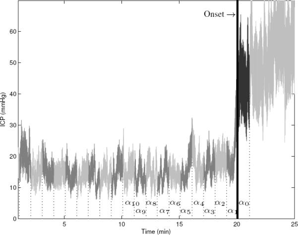
Illustration of an elevated ICP episode (IH), from our dataset $\mathcal{D}$. Elevated episodes are divided into 21 segments of 1-minute length. For each segment, MOCAIP is applied to extract a representative ICP pulse using hierarchical clustering and morphological vectors α are calculated.

2.3. Experimental Setup

The prediction of ICP elevation on our dataset is posed as a classification problem where each input example x_i ∈ X; is a set of ${\mathcal{N}}_s$ MOCAIP vectors $x_i=\{{\alpha }_0,\dots ,{\alpha }_{{\mathcal{N}}_s-1}\}$ calculated over a series of successive one-minute ICP segments. The corresponding output y_i ∈ Y is a binary variable which equals 1 if the ICP segment led to a treated IH episode. The performance in terms of Area Under the Curve (AUC), sensitivity, and specificity (Section 2.3.1) are reported for input segments x_i extracted at various time-to-onset for the Linear, AdaBoost, and Extra-Trees predictive models described in Section 2.4. A comparative analysis is provided in Section 2.3.2 between models trained over 24-dimensional MOCAIP vectors (to describe each 1-min segment) versus models trained from a subset (< 24) of the metrics selected after sequential feature selection. In Section 2.3.3, the impact of the number ${\mathcal{N}}_s$ of successive ICP segments used to construct the input vectors $x_i=\{{\alpha }_0,\dots ,{\alpha }_{{\mathcal{N}}_s-1}\}$ is evaluated for each prediction technique. The main purpose of the experiment is to test the hypothesis that the use of ensemble classifiers improves the prediction of IH because it can exploit more efficiently the morphological information contained in longer ICP segments located prior to the elevation onset. This would also indicate that consecutive ICP waveforms extracted prior to the elevation hold complementary precursors of IH.

2.3.1. Performance Evaluation by Time-To-Onset Variation

For evaluation, a ten-fold cross-validation is performed such that at each iteration, nine folds are used to train the model while the remaining one is retained for testing. The partitioning is randomly made at the patient level; with the constraint that the pulses of a given patient are grouped into the same fold. This ensures that the data from a given patient are not present at the same time in the training and testing sets.

Linear, AdaBoost, and Extra-Trees models are trained on each fold such that each positive example $x_i=\{{\alpha }_0,\dots ,{\alpha }_{{\mathcal{N}}_s-1}\}$ corresponds to the ${\mathcal{N}}_s-1$ vectors of morphological metrics ${\alpha }_i\in {\mathbb{R}}^{{\mathcal{N}}_f}$ extracted immediately prior to onset plus the one at onset. The negative examples are randomly sampled from the pulses of the control set such that the training dataset is balanced and contains an equal number of positive and negative examples. For testing, the models are evaluated on the excluded fold by varying the time-to-onset ρ at which the ICP segments $x_i=\{{\alpha }_{0{+}_{\rho }},\dots ,{\alpha }_{{\mathcal{N}}_s-1{+}_{\rho }}\}$ are extracted. For fair comparison, the control episodes used for testing the model at the different time-to-onset remain the same for each run.

Predictions are evaluated at each time-to-onset using a receiver operating characteristic (ROC) analysis [26] from which sensitivity and specificity are computed at a specific threshold. In addition, the AUC is used to measure the classification performance; it represents the probability of correct classification for a randomly chosen pair of positive and negative examples.

2.3.2. Feature Selection

Feature selection was shown in a previous study [11] to improve the prediction of IH for individual classifiers. We perform a similar experiment to replicate these results on our dataset in terms of AUC and to see if they lead to similar improvements for ensemble classifier methods.

A backward sequential feature selection scheme is used, starting with the full set of ${\mathcal{N}}_f=24$ morphological features to describe each 1-min segment and then removing one feature at a time. At each iteration, the feature to be removed is chosen so that it maximizes the average AUC computed over ten different time-to-onset ρ = {0, … , 9} ranging from zero to nine minutes. The selection process stops when no further improvement can be achieved by removing any of the features. For this experiment, models were trained using positive examples corresponding to a single${\mathcal{N}}_s=1$ 1-min morphological vector α₀ concurrent to the elevation onset, and 1-min control ICP segments randomly extracted from the current fold.

2.3.3. Number of Morphological ICP Segments

This experiment aims at evaluating if the use of additional morphological vectors extracted up to ten minutes $({\mathcal{N}}_s=10)$ prior to the tested time-to-onset can improve the prediction performance of the models. To do so, linear and ensemble classifiers (AdaBoost, and Extra-Trees) are trained such that the input x_i of the positive examples are the ${\mathcal{N}}_s$ morphological vectors $\{{\alpha }_0,{\alpha }_1,\dots ,{\alpha }_{{\mathcal{N}}_s-1}\}$ extracted from the segments prior to the onset plus the segment concurrent to the IH onset, as illustrated in Figure 3. Training of the models is performed for ten different lengths ${\mathcal{N}}_s=\{1,\dots ,10\}$, from one to ten minutes. Controls of corresponding lengths are randomly extracted from the current fold but remain the same across the different time-to-onset. Similarly to the previous experiments, each model is evaluated using the average AUC results computed from a ten-fold cross-validation, and ten different time-to-onset ρ = {0, … , 9}.

Figure 3.

MOCAIP splits the raw ICP signal into individual pulses using ECG and clusters them so that an average representative pulse is extracted from each one-minute segment. Then peaks are detected, morphological vectors α are computed and used as input to the ensemble classifiers to make prediction about future ICP elevation.

2.4. ICP Prediction Techniques

Three different prediction techniques are evaluated in our experiments. They are based respectively on Multiple Linear Regression (MLR), and two ensemble classifiers techniques; Adaptive Boosting (AdaBoost), and Extremely Randomized Decision Trees (Extra Trees) that are described below.

The data used to train the three algorithms is denoted {X, Y } where X is a set of n input examples $x_i\in {\mathbb{R}}^{{\mathcal{N}}_s\times {\mathcal{N}}_f}$ and Y the corresponding set of class labels y_i ∈ 0, 1 which equals 1 if the segment was extracted from an elevated episode, and 0 otherwise.

2.4.1. Multiple Linear Regression

A common way to obtain a regression model is to perform a Multiple Linear Regression analysis [5]. The intuition behind this technique is to fit a model such that the sum-of-squares error (SSE) between the observed and the predicted values is minimized.

Let β a matrix of s parameters, the model is written:

$$Y=\beta X+∊$$ (1)

$$\iff y_i={\beta }_1{x}_i\left(1\right)+{\beta }_2{x}_i\left(2\right)+\dots +{\beta }_s{x}_i\left(s\right)+{∊}_i$$ (2)

where i = 1 … n and ∊_i = N(0, σ²) denotes a set of noise variables.

Multiple Linear Regression analysis finds estimates coefficients $\widehat{\beta }$ such that they minimize the sum-of-squares error (SSE) which measures the total error between each prediction and the actual value of the output variable,

$$\widehat{\beta }={\mathrm{argmin}}_{\beta }\sum _{i=1}^n{(\beta x_i-y_i)}^2$$ (3)

The optimal $\widehat{\beta }$ can be expressed as $\widehat{\beta }={\left(X{X}^T\right)}^{-1}{X}^{T}Y$. We used a QR factorization to obtain estimated regression coefficients $\widehat{\beta }$.

2.4.2. Adaboost Classifier

Adaptive Boosting [21], or AdaBoost, is a machine learning algorithm to improve the performance of simple classifiers by combining several of them into a single, more accurate ensemble classifier. The individual classifiers are called weak classifiers because they are only required to perform better than chance at each successive iteration of the algorithm.

The AdaBoost algorithm, as presented in Algorithm 1, trains each weak classifier c_l=1…L sequentially, so that each of them c_l is trained on the same data but observations that were misclassified by preceding weak classifiers are associated with a larger weight p_l. In this work, each classifier works as a simple threshold on the input features.

Algorithm 1.

AdaBoost Algorithm

// Initialize weigths for all data points

w1(i) ← 1/n, ∀i ∈ {1, …, n}

for l=1 to L do

// Normalize weights

$p_l\left(i\right)\leftarrow w_l\left(i\right)∕{\Sigma }_{i=1}^n{w}_l\left(i\right),{\forall }_i\in \{1,\dots ,n\}$

// Learn weak classifier

cl ← weakLearn(X, Y, pl)

// Computer error

${\epsilon }_l\leftarrow {\Sigma }_{i=1}^n{p}_l\left(i\right)\mid c_l\left(x_i\right)-y_i\mid$

if εl < 0.5 then

L ← l − 1

break

end if

// Update parameters

βl ← εl/(1 − εl)

$w_{l+1}\left(i\right)\leftarrow w_l\left(i\right){\beta }_l^{1-[c_l\left(x_l\right)-y_l]}$

end for

$\widehat{y}\leftarrow {\Sigma }_{l=1}^L\log \left({\beta }_l^{-1}\right){\mid c_l\left(x\right)-1\mid }^{-1}$

The final classifier, c, is constructed by a weighted vote of the L weak classifiers c₁, c₂, … c_L. Each classifier is weighted according to its accuracy for the weight distribution p_l that it was trained on.

2.4.3. Extremely Randomized Decision Trees

Classification and regression trees have recently become a method of choice to build predictive models. Their versatility and intuitive interpretation make them particularly suitable for biomedical applications. The sequence of rules learned by the models can be extracted easily and visualized graphically. This is an important feature to consider since it could ultimately be delivered to bedside clinicians.

In this work, we use Extremely Randomized Decision Trees (Extra-Trees) [7]. It is an ensemble classifier method that extends conventional decision trees by introducing randomness during the construction process. During learning, an ensemble of randomized trees is constructed in a supervised way and later used to predict the output of previously unseen input vectors. During training, several trees are constructed from the dataset {X, Y} of the s-dimensional input examples $x_i\in {\mathbb{R}}^s$ and their corresponding output y_i ∈ {0, 1}. The procedure to build an Extra-Tree works in a recursive fashion by successively splitting the nodes where the output varies, as described in Algorithm 2. At each successive node, candidate thresholds {λ₁, …, λ_s} are generated randomly (within the range of the data) for each of the s input attributes of X. Each candidate threshold λ is used to split the data {X, Y} into two subsets {X_l, Y_l}, {X_r, Y_r}, and it is then associated with a score ψ_λ (Eq. (4)) based on the relative variance reduction,

$${\psi }_{\lambda }=\frac{\mathrm{var}\left(Y\right)-\frac{\mid Y_l\mid }{\mid X\mid }\mathrm{var}\left(Y_l\right)-\frac{\mid Y_r\mid }{\mid X\mid }\mathrm{var}\left(Y_r\right)}{\mathrm{var}\left(Y\right)},$$ (4)

where |X| denotes the length of the vector X and var(Y) is the variance of the output available at the current node. The threshold with the highest score is used to annotate the current node and the two resulting subsets {X_l, Y_l}, {X_r, Y_r} are used as input data for constructing the left t_l and the right t_r subtrees, respectively. The construction process continues for all the nodes that have at least n_min = 5 samples (as suggested in [7]) and where the output varies across training samples. During prediction, the input vector x_i is processed by all the trees. The outputs of the trees are aggregated and the average yields the final prediction ŷ_i.

Algorithm 2.

t = buildExtraTree(X, Y)

if |X| < nmin OR isConstant(Y) then

Return buildLeaf(mean(Y))

end if

// Generate Candidate Thresholds at Random

{λ1, …, λn} ← GenerateSplits(min(X(j)),max(X(j))), ∀j ∈ {1, …, s}

// Select Threshold with Best Score (Eq. (4))

${\lambda }_j\leftarrow \underset{j}{\arg \max }{\psi }_{{\lambda }_j}\left(X\right)$

// Split Data, Recurse, and Build node

{Xl, Yl, Xr, Yr} ← λj(X, Y)

tl ← buildExtraTree(Xl, Yl)

tr ← buildExtraTree(Xr, Yr)

Return buildNode(λj, j, tl, tr)

3. Results

Results of the feature selection experiment are illustrated in Figure 4 for the linear classifier. The performance of the linear models using the original set of 24 MOCAIP metrics are depicted by a dashed line. It reflects the AUC computed for time-to-onset varying from zero to ten minutes. After a sequential feature selection procedure, 13 features (lt, l2, l3, l12, l13, dp12, dp23, dp3, curv1, curv3, curv12, curv13, curv23, tcurv) were found to lead to the best accuracy in terms of AUC. The results of the linear model after sequential feature selection are depicted by solid lines. Values of the AUC at the time-to-onset [1, 3, 6] mins are [0.76, 0.66, 0.58] for the full set of 24 features, and [0.87, 0.78, 0.71] for the best 13 MOCAIP metrics. Improvements of similar orders were observed in terms of sensitivity; from [0.70, 0.56, 0.45] to [0.76, 0.62, 0.52], specificity; from [0.64] to [0.72]. Note that specificity remains constant because for fair comparison the set of controls remain the same for the different time-to-onset. Therefore, the number of true negative and false positive cases does not change, which in turn leads to a constant specificity. While the mean ICP is certainly a useful feature to detect the elevation during the ascending phase of the ICP immediately prior to the onset, it seems to mislead the linear classifier to predict IH at earlier times. When averaging the classification results over the 10 different time-to-onset the use of mICP leads to a decrease of the performances. This can be explained by the fact that we are considering plateau waves that present a sharp increase in ICP. For example, several minutes prior to the elevation onset, the mean ICP may actually be higher on some control episodes and may therefore confuse the training of the linear classifier.

Figure 4.

Illustration of the AUC (a), Sensitivity (b), and Specificity (c) for the multi-linear classifier using the ${\mathcal{N}}_f=24$ morphological metrics versus a subset of of ${\mathcal{N}}_f=13$ features selected using a sequential feature selection procedure. Results are reported for different time-to-onset values (ρ ∈ 2 [0, 10]) for models trained on a single vector $({\mathcal{N}}_s=1)$. All the performance metrics are improved using the feature subset.

No performance improvement in terms of AUC could be obtained via sequential feature selection for AdaBoost and Extra-Trees. The lack of performance increase could be attributed to a nonlinear relationship between some of the morphological features of ICP and the occurrence of an IH episode. By removing these features using feature selection, we could improve the overall accuracy of the linear model although it was still significantly lower than the results obtained by the ensemble classifiers.

Figure 5 illustrates the results obtained by the three methods after varying the number ${\mathcal{N}}_s$ of one-minute segments used as input from one to ten. The Extra-Trees method shows significant improvement in terms of average AUC when the length of the input is increased. For [1, 5, 10] minute(s)-long segments, the AUC is respectively [0.77, 0.88, 0.9]. AdaBoost also shows significant increases in AUC, from [0.75, 0.83, 0.84] for segments of [1, 5, 10] minute(s) length, respectively. The linear models are unable to efficiency exploit the larger segments of morphological ICP data. AUC results are [0.76, 0.65, 0.73] for segments of [1, 5, 10] minute(s) length, respectively. The best average AUC for the linear model was observed using a single ICP segment ${\mathcal{N}}_s=1$. In contrast, the best performance for AdaBoost and Extra-Trees models is obtained with ${\mathcal{N}}_s=10$ ICP segments, corresponding to ten minutes of ICP data extracted prior to the tested time-to-onset. These results seem to indicate that the relationship between ICP morphology and future elevation is not easily captured by a linear model.

Figure 5.

Illustration of the AUC after a leave-one-out crossvalidation for the Extra-Trees (a), AdaBoost (b), and multi-linear classifier (c). Results are reported for models trained with different length of the ICP segment prior to the time the prediction is made. Ensemble classifiers (AdaBoost and Extra-Trees) are able to exploit a longer sequence in comparison with the multi-linear classifier.

The best results of each method are reported in Figure 6 in terms of AUC, sensitivity, and specificity. While the linear classifiers obtain an AUC of [0.87, 0.78, 0.71] for the time-to-onset corresponding to [1, 3, 6] minutes prior to the elevation respectively, the use of ensemble classifiers significantly improves the AUC. AdaBoost reaches an AUC [0.93, 0.84, 0.80], and Extra-Trees performs even better with an AUC of [0.96, 0.91, 0.87]. Improvements can also be observed in terms of sensitivity; where Extra-Trees obtain [0.93, 0.83, 0.75], AdaBoost follows with [0.90, 0.71, 0.65], and linear stays behind [0.76, 0.62, 0.52]. These results were obtained at a specificity of [0.98, 0.93, 0.72], for Extra-Trees, AdaBoost, and linear methods respectively. It should be acknowledged that the experimental protocol used in this study does not evaluate the power of the model to predict temporal raise of ICP se at the patient level (which would be required for integration on a bedside monitor), but rather reflects the feasibility of using the morphological information of ICP waveforms to classify the segment on the basis of an imminent plateau waves (within the next 10 mins). The good performance can in part be attributed to the difference between the patients who had at least an IH episodes and the ones who did not. To study this point deeper, we measured the specificity within the two populations of controls (IH or not), as shown below,

	Non-IH Control	IH Control	All Controls (Fig. 6)
Linear	.73	.72	.72
Adaboost	.97	.76	.93
Extra-Trees	.99	.96	.98

As expected, the specificity is lower for controls with at least one IH episodes. The difference for Adaboost is large (.21), while there is a much smaller difference for the Linear classifier (.01) and Extra-Trees (.03). Note that the sensitivity (TP / (TP+FN)) is not affected by the population of control cases during evaluation.

Figure 6.

Illustration of the AUC (a), Sensitivity (b), and Specificity (c) after a leave-one-out crossvalidation for the multi-linear classifier, AdaBoost, and Extra-Trees. The multi-linear utilizes the optimal subset of 13 morphological features, while AdaBoost and Extra-Trees use the 24 metrics. Extra-trees performance ranks best and is followed by the AdaBoost and Multi-linear classifier.

Although the previous experiments (Figure 5) demonstrate that the ensemble classifier models trained over 10 minutes of ICP data perform better than the one trained over shorter segments, it is not clear if each additional one minute ICP segment contribute independently to the improvements, or if they are complementary; in which case the dynamic of change of ICP morphology over time would appear to be useful. To test these hypothesis, three different learning strategy of the Extra-Trees models are compared. The first model (a), which is used as baseline, is trained on a single (${\mathcal{N}}_s=1$) one-minute long segment x_i = {α₁}. The second strategy (b) consists in learning independently ten different models on each one-minute long segment and then fuse their output using an arithemic mean. Finally, the last one (c) is to build a single model trained on a series of ten (${\mathcal{N}}_s=10$) one-minute long segments concatenated to a single input vector x_i = {α₁, …, α₁₀}. Results after a leave-one-out crossvalidation are reported in Figure 7 in terms of the AUC at different time-to-onset. Although, the use of ten independent classifiers (b) improves the overall performance versus the use of only one classifier (a), there is an additional increase in AUC by using all ten vectors at the same time (c). This results indicates that the relative values of successive morphological vectors contain relevant precursors of IH. It is an important finding because it means that the dynamic of ICP changes holds critical predictive information.

Figure 7.

Illustration of the Area Under the Curve (AUC) after a leave-one-out crossvalidation for three different learning strategy of the Extra-Trees models. The first model is trained on a series of 10 one minute long segments concatenated to a single input vector x_i = {α_1+ρ, …, α_10+ρ}. The second strategy consists in learning ten different models on each one minute long segment and then fuse their output using an arithmetic mean. Finally, the last one is build a single one minute long length segment x_i = {α_0+ρ}. Al-though, the use of 10 individual classifier improves the overall performance, an additional increase in AUC is observed by using all the 10 vectors at the same time. This indicates that the relative values of successive morphological vector contain relevant precursors of IH.

Because 50 decision trees have been used to construct each Extra-Trees model in our experiments, they cannot directly be translated into simple rules. Additional work is required to simplify these models to make them accessible and understandable by bedside clinicians. An Extra-Tree constructed during our experiments on 24 MOCAIP features is illustrated in Figure 8 where Nj denotes the feature to be tested in the current node. The test of each node is shown inside the ellipsis. Starting with an input vector x_i at the root of the tree, the process follows the right branch if the test is true, otherwise it follows the left branch. The process stops when it reaches a leaf and the corresponding annotation (0, or 1) of the leaf is returned as the predicted output ŷ_i.

Figure 8.

Example of Extra-Tree constructed during our experiments from 24 × 10 MOCAIP features. During prediction, the MOCAIP features of a given input vector x_i denoted Nj (where j is the index of the feature) are successively tested at each node. The test of each node is shown inside the ellipsis. If the test is true, it proceeds on the right, otherwise it proceeds on the left branch. The process stops when it reaches a leaf, represented by square rectangles, and the corresponding annotation of the leaf is returned as the predicted output ŷ_i.

4. Discussion

The present study expands on previous works [8, 11] regarding the development of predictive algorithms of acute ICP elevation. A novel methodological and experimental framework have been designed to evaluate predictions made by multiple linear and ensemble classifiers (based on AdaBoost and Extra-Trees).

While the multiple linear classifier applied on 1-minute ICP segments shows signs of predictivity five minutes before elevation onset when trained on an optimal subset of morphological features of the ICP, the sensitivity (60%) and specificity (70%) reached by the model remains too low to meet the performance requirements of a clinical environment. Thanks to the use of a series of successive 1-minute ICP segments as input to classifier ensemble techniques, the proposed study has demonstrated that they can exploit more efficiently the morphological information contained in the pulse. Ensemble classifiers used within our framework significantly improve the results obtained by a linear model both in terms of specificity and sensitivity on our dataset. The AUC is above 85%, which corresponds to the probability of the algorithm to be correct for a random pair of positive and negative samples. The performance improvement observed in our experiments can be attributed to the three main following reasons:

• First, as it has been shown in other applications, the two ensemble classifiers perform better than the multiple linear classifier because they can better capture the nonlinearity between the morphological vectors and the outcome.

• Second, the use of a larger segment of ICP segment prior to the onset, represented as a series of morphological vectors, also improves the accuracy because the additional information contained in earlier vectors is useful to discriminate between IH and controls episodes.

• Finally, the use of a full sequence of successive morphological vectors at once for the learning leads to better models than the one trained on each morphological vector individually. This means that the relative values and the order between successive morphological vectors, and therefore the morphological dynamics of ICP, contain additional precursors of IH.

While the performance reached by our framework may help the bedside clinician to react more quickly to prevent occurance of certain types of IH, the treatment of TBI patients may lead to additional challenges and require earlier predictions. For those patients, a multi-modal approach combining images, ABP, and TCD measurements may help to identify patients with greater risks of future IH episdes well before the 10 mins windows used by the current model.

Although the ICP of brain injured patients is continuously managed by the bedside clinicians, changes in ICP prior to elevation are reflected by complex variations in the morphology of the signal that are difficult to be recognized in real-time. Decision support tools that would alert the bedside clinicians of future ICP elevation would add a new proactive dimension to the current treatment of ICP elevations, which largely remains a reactive procedure. Future studies will investigate the proposed framework for brain injury patients. Such studies are needed before generalizing our results because these patients are likely to have specific pathological mechanisms behind ICP elevation and therefore differ from the ICP elevation in the patients studied in this paper.

Further improvement of the technical methodology and a better understanding of the physiological meaning of these morphological variations should be possible. Ideally, we would like to translate the rules learned by ensemble classifiers into a physiological model in an attempt to represent ICP dynamics explicitly. Although we were able to illustrate a few rules obtained from the decision trees, additional work is required to interpret those models from a physiological point of view, such findings would be a breakthrough in the understanding of ICP dynamic prior to acute elevation.

In previous studies of ICP elevation predictors [8, 11], morphological features were extracted using three minutes segments to avoid the effect of noise and artifacts that typically occur during ICP recording. In this work, thanks to recent improvements in the morphological description of ICP, a finer resolution of one minute was used to extract the morphological features. Such a resolution may still be a limiting factor of the study. Shorter-term variations of ICP might hold relevant precursors of future elevations. A beat-by-beat analysis of ICP metrics would be ideal. We are currently developing an ICP tracking analysis framework that will perform at the beat level, which would be a significant step towards real-time ICP elevation prediction.

References

- [1].Afonso VX, Tompkins WJ, Nguyen TQ, Luo S. Ecg beat detection using filter banks. IEEE Trans Biomed Eng. 1999;46(no. 2):192–202. doi: 10.1109/10.740882. [DOI] [PubMed] [Google Scholar]
- [2].Allen R. Time series methods in the monitoring of intracranial pressure. J Biomed Eng. 1983;5:5–18. doi: 10.1016/0141-5425(83)90073-0. [DOI] [PubMed] [Google Scholar]
- [3].Asgari S, Xu P, Bergsneider M, Hu X. A subspace decomposition approach toward recognizing valid pulsatile signals. Physiol Meas. 2009 Nov;30:1211–1225. doi: 10.1088/0967-3334/30/11/006. [DOI] [PMC free article] [PubMed] [Google Scholar]
- [4].Azzerboni B, Finocchio G, Ipsale M, Forestal FL, Morabito F. Intracranial pressure signals forecasting with wavelet trasform and neuro-fuzzy network. Proceedings of the second joint EMBS-BMES conference; Houston, TX, USA. 2002. pp. 1343–1345. [Google Scholar]
- [5].Chatterjee S, Hadi AS. Influential observations, high leverage points and outliers in linear regression. Statistical Science. 1986;1:379–393. [Google Scholar]
- [6].Czosnyka M, Smielewski P, Piechnik S, Schmidt EA, Al-Rawi PG, Kirkpatrick PJ, Pickard JD. Hemodynamic characterization of intracranial pressure plateau waves in headinjured patients. J. Neurosurg. 1999;91(no. 1):11–19. doi: 10.3171/jns.1999.91.1.0011. [DOI] [PubMed] [Google Scholar]
- [7].Geurts P, Ernst D, Wehenkel L. Extremely randomized trees. Mach Learn. 2006;63(no. 1):3–42. [Google Scholar]
- [8].Hamilton R, Xu P, Asgari S, Kasprowicz M, Vespa P, Bergsneider M, Hu X. Forecasting intracranial pressure elevation using pulse waveform morphology. Proceedings of the IEEE Engineering in Medicine and Biology Society (EMBS); Minneapolis, MN, USA. 2009. pp. 4331–4334. [DOI] [PubMed] [Google Scholar]
- [9].Hornero R, Aboy M, Abasolo D, McNames J, Goldstein B. Interpretation of approximate entropy: analysis of intracranial pressure approximate entropy during acute intracranial hypertension. IEEE Trans Biomed Eng. 2005;52(no. 10):1671–80. doi: 10.1109/TBME.2005.855722. [DOI] [PubMed] [Google Scholar]
- [10].Hu X, Miller C, Vespa P, Bergsneider M. Adaptive computation of approximate entropy and its application in integrative analysis of irregularity of heart rate variability and intracranial pressure signals. Med Eng Phys. 2008 Jun;30:631–639. doi: 10.1016/j.medengphy.2007.07.002. [DOI] [PMC free article] [PubMed] [Google Scholar]
- [11].Hu X, Xu P, Asgari S, Vespa P, Bergsneider M. Forecasting icp elevation based on prescient changes of intracranial pressure waveform morphology. IEEE Trans Biomed Eng. 2010;57(no. 5):1070–1078. doi: 10.1109/TBME.2009.2037607. [DOI] [PMC free article] [PubMed] [Google Scholar]
- [12].Hu X, Xu P, Lee D, Vespa P, Bergsneider M. An algorithm of extracting intracranial pressure latency relative to electrocardiogram r wave. Physiol Meas. 2008;29:459–471. doi: 10.1088/0967-3334/29/4/004. [DOI] [PMC free article] [PubMed] [Google Scholar]
- [13].Hu X, Xu P, Scalzo F, Vespa P, Bergsneider M. Morphological Clustering and Analysis of Continuous Intracranial Pressure. IEEE Trans Biomed Eng. 2009;56(no. 3):696–705. doi: 10.1109/TBME.2008.2008636. [DOI] [PMC free article] [PubMed] [Google Scholar]
- [14].McNames J, Crespo C, Bassale J, Aboy M, Ellenby M, Lai S, Goldstein B. Sensitive precursors to acute episodes of intracranial hypertension. 4th International Workshop Biosignal Interpretation.2002. pp. 303–306. [Google Scholar]
- [15].Piper I, Miller J, Dearden M, Leggate J, Robertson I. Systems analysis of cerebrovascular pressure transmission: An observational study in head-injured patients. J Neurosurg. 1990;73:871–880. doi: 10.3171/jns.1990.73.6.0871. [DOI] [PubMed] [Google Scholar]
- [16].Portnoy HD, Chopp M. Cerebrospinal fluid pulse wave form analysis during hypercapnia and hypoxia. Neurosurg. 1981;9(no. 1):14–27. doi: 10.1227/00006123-198107000-00004. [DOI] [PubMed] [Google Scholar]
- [17].Price D, Dugdale R, Mason J. The control of icp using three asynchronous closed loop. Intracranial Pressure IV. 1980:395–399. [Google Scholar]
- [18].Rosner M. Pathophysiology and management of increased intracranial pressure. Neurosurgical Intensive Care. 1993:57–112. [Google Scholar]
- [19].Scalzo F, Asgari S, Kim S, Bergsneider M, Hu X. Robust peak recognition in intracranial pressure signals. Biomed Eng Online. 2010;9(no. 61) doi: 10.1186/1475-925X-9-61. [DOI] [PMC free article] [PubMed] [Google Scholar]
- [20].Scalzo F, Xu P, Asgari S, Bergsneider M, Hu X. Regression analysis for peak designation in pulsatile pressure signals. Med Biol Eng Comput. 2009;47(no. 9):967–977. doi: 10.1007/s11517-009-0505-5. [DOI] [PMC free article] [PubMed] [Google Scholar]
- [21].Schapire RE. The strength of weak learnability. Mach. Learn. 1990 Jul;5:197–227. [Online]. Available: http://portal.acm.org/citation.cfm?id=83637.83645. [Google Scholar]
- [22].Swiercz M, Mariak Z, Krejza J, Lewko J, Szydlik P. Intracranial pressure processing with articial neural networks: Prediction of icp trends. Acta Neurochir (Wien) 2000;142(no. 4):401–406. doi: 10.1007/s007010050449. [DOI] [PubMed] [Google Scholar]
- [23].Szewczykowski J, Dytko P, Kunicki A, Korsak-Sliwka J, Sliwka S, Dziduszko J, Augustyniak B. Determination of critical icp levels in neuro-surgical patients: A statistical approach. Intracranial Pressure II. 1975:392–393. [Google Scholar]
- [24].Tsui F-C, Sun M, Li C-C, Sclabasi R. A wavelet based neural network for prediction of icp signal. IEEE EMBC. 1995:1045–1046. [Google Scholar]
- [25].Turner J, McDowall D, Gibson R, Khaili H. Computer analysis of intracranial pressure measurements: Clinical value and nursing response. Intracranial Pressure III. 1976:283–287. [Google Scholar]
- [26].Zweig MH, Campbell G. Receiver-operating characteristic (ROC) plots: a fundamental evaluation tool in clinical medicine. Clinical chemistry. 1993 Apr;39(no. 4):561–577. [Online]. Available: http://view.ncbi.nlm.nih.gov/pubmed/8472349. [PubMed] [Google Scholar]